Specific Emitter Identification Based on the Natural Measure

Abstract

Specific emitter identification (SEI) techniques are often used in civilian and military spectrum-management operations, and they are also applied to support the security and authentication of wireless communication. In this letter, a new SEI method based on the natural measure of the one-dimensional component of the chaotic system is proposed. We find that the natural measures of the one-dimensional components of higher dimensional systems exist and that they are quite diverse for different systems. Based on this principle, the natural measure is used as an RF fingerprint in this letter. The natural measure can solve the problems caused by a small amount of data and a low sample rate. The Kullback–Leibler divergence is used to quantify the difference between the natural measures obtained from diverse emitters and classify them. The data obtained from real application are exploited to test the validity of the proposed method. Experimental results show that the proposed method is not only easy to operate, but also quite effective, even though the amount of data is small and the sample rate is low.

1. Introduction

Recently, in Electronic Warfare (EW) and Electronic Intelligence (ELINT) systems [1], distributed detection of a non-cooperative target [2], distributed modulations classification [3], and specific emitter identification (SEI) have attracted much attention. The SEI technique was first proposed in the mid-1960s for identifying and tracking specific transmitters. This technique discriminates the individual transmitter of a given signal by comparing the features carried by the signal with a library of feature sets, and selecting the most matchable class [4]. SEI techniques can be used to support the applications of wireless communication security and authentication [5,6]. In SEI systems, the identification concerns particular emitter copies of the same type classification, while recognition concerns only emitter types classification and is not as advanced as identification.

The key to any SEI system is the useful feature sets obtained from the signal that make identification possible [4]. Thus, the most important thing is to extract the valid RF fingerprints of a given signal when implementing an effective SEI system. Generally, SEI techniques can be divided into two broad categories: radar signal-based SEI and communication signal-based SEI, according to different application scenarios and the characteristics of signals. However, some SEI methods can be used in both radar signals and communication signals.

In the case of radar signals, SEI techniques are always based on the intra-pulse analysis [7], the use of out-of-band radiation [8], the theory of fractals [9], the graphical representation of the distribution of radar signal parameters [10], the use of the agglomerative method of hierarchical radar signal clustering [11], the Wigner–Ville distribution (WVD) [12], etc.

In the case of communication signals, SEI techniques can be divided into three categories: transient signal techniques, steady-state signal techniques, and nonlinear techniques. A transient signal is actually a brief radio emission produced while the output power of a transmitter goes from zero to the level required for data communication. A steady state signal is usually defined as the part between the end of the transient and the end of the whole signal.

In transient analysis, the RF fingerprints are always extracted from instantaneous amplitude, phase, and frequency of the received signals due to the difference caused by the idiosyncratic characteristics of power amplifiers, filters, and frequency synthesizers. Recent research has shown that the transient-based SEI techniques have good classification performance [13,14]. However, the duration of transient signals are quite short, and there is not enough data for RF fingerprint extraction and identification. The analysis based on the transient signal also needs very high sample rates, which makes the architecture of the receiver complex. The identification of the emitters which are from the same manufacturer may require a high-end receiver to offer a high oversampling rate to detect the transient signals [15].

In contrast with the works of transient analysis, the steady response approaches are more practical. There are many SEI techniques which are based on the analysis of steady response, including modulation-based method, spectrum-based method, transform-based method, and so on. Recently, Brik et al. developed a modulation-based method to extract the RF fingerprints from a steady-state signal, and achieved the identification accuracy of 99% [16]. Scanlon et al. applied the spectral averaging technique to the SEI and achieved the identification accuracy of 99.8% [17]. However, these methods [16,17] are performed under the condition that the transmitters and the receivers are located in an anechoic chamber, whereas the receivers are usually as far as several kilometers from the transmitters in practice. The transform-based method (e.g., the method based on the wavelet packet decomposition) has been studied for a long time [18], but its performance is usually affected by the selection of the basis of the transformation.

The nonlinear techniques can be divided into two groups: the techniques based on nonlinear characteristics and the techniques based on nonlinear modeling. Carroll has demonstrated the validity of exploring the nonlinearity of amplifiers for signal identification [19]. His method is based on the phase space analysis, and it usually needs a lot of data to obtain reliable results. Huang et al. extracted the normalized permutation entropy (NPE) as the RF fingerprint to identify the unique transmitter, and achieved a relatively good performance [20]. However, the embedding dimension should be determined first, and the amount of data to calculate the NPE should be large if one wants to obtain a relatively reliable statistic. Polak et al. identified the unique emitter by modeling the nonlinearity of power amplifier (PA) and integral nonlinearity (INL) of the digital-to-analog converter (DAC) with Volterra series and a Brownian Bridge random process, respectively [21]. Its performance would become worse when these models do not match well with the real signals. Zhang et al. proposed another SEI method based on the nonlinear modeling and the Hilbert–Huang Transform (HHT) [22] in the case of relaying scenario and single-hop scenario. Obviously, the accuracy of the model will affect the performance of this type of approach.

As demonstrated by Carroll, the amplifiers are inherently nonlinear because they depend on semiconductors [19]. As a result, one can study the communication transmitters, as they are dynamical systems. The signals from actual communication transmitters can be considered nonlinear, since the nonlinear property of such transmitters will be translated in the signals. Thus, we can extract the RF fingerprints from received signals from the nonlinear point of view. In consideration of the drawbacks of the aforementioned nonlinear SEI approaches [20,21,22], we will propose a novel nonlinear SEI method based on the natural measure of the one-dimensional component of higher dimensional systems. This method does not need any model, and it is effective in the case of a relatively small amount of data and low sample rate.

2. Proposed Method

The method proposed in this letter is based on treating the communication transmitter as a nonlinear dynamical system. Based on this principle, the natural measure of the received signal is extracted and used as an RF fingerprint. In fact, the natural measure is a useful tool that helps us to better understand chaotic maps or systems. Before introducing the concept of the natural measure, another related concept called natural invariant density should be introduced first.

For a one-dimensional chaotic map defined on $\left[0,1\right]$, its natural invariant density can be defined as follows. For any given interval $\left[a,b\right]\subset \left[0,1\right]$, if the fraction of time that typical orbits fall into the interval $\left[a,b\right]$ is ${\int }_a^b\rho \left(x\right)dx$, then the function $\rho \left(x\right)$ will be called the natural invariant density of this one-dimensional chaotic map. As an example, the logistic map with $r=4$ (shown in Equation (1)) and its natural invariant density $\rho \left(x\right)$ [23] (shown in Equation (2)) are shown as follows:

$$x_{n+1}=r{x}_n\left(1-x_n\right)$$

(1)

$$\rho \left(x\right)=\frac{1}{\pi \sqrt{x\left(1-x\right)}}$$

(2)

Compared to the natural invariant density, the natural measure is more practical [23]. For the chaotic attractor of a one-dimensional map, its natural measure can be defined as follows. Let A be an interval in the phase space; let $x_0$ be an initial value in the basin of attraction of the chaotic attractor B; let $x\left(t,x_0\right)$ be the orbit generated by the initial value $x_0$; and let $\mu \left(A;x_0,T\right)$ be the fraction of time that $x\left(t,x_0\right)$ spends in A in the time interval $0\le t\le T$, and assume that the limit in Equation (3) exists.

$$\mu \left(A;y_0\right)=\underset{T\to \infty }{lim}\mu \left(A;y_0,T\right)$$

(3)

If $\mu \left(A,x_0\right)$ stays unchanged for every $x_0$ in B except for a set of $x_0$-values of Lebesgue measure zero, then $\mu \left(A,x_0\right)$ is the natural measure of A and can be denoted as $\mu \left(\mathrm{A}\right)$. For more details about the natural invariant density and the natural measure, please see Ref. [23]. For a received signal $x_t,t=1,2,\cdots ,N$, its natural measure can be evaluated as follows:

1

Normalizing the signal to $[0,1]$:

$${\tilde{x}}_t=\frac{x_t-min\left(x_t\right)}{max\left(x_t\right)-min\left(x_t\right)}$$

(4)

2

Equally dividing the interval $[0,1]$ into L parts $\left(\left(i-1\right)\Delta ,i\Delta \right],i=1,2,\cdots ,L$, according to a given length of the inter-cell Δ, where $L=⌊1/\phantom{1\Delta }\Delta ⌋$ is the integer smaller than or equal to $1/\phantom{1\Delta }\Delta$. The midpoint of each inter-cell will be the representative point.

3

Calculating the probability $p_i$ where the data fall into the interval $\left(\left(i-1\right)\Delta ,i\Delta \right]$;

$$p_i=\frac{\#\left\{{\tilde{x}}_t\left|1\le t\le N,\left(i-1\right)\Delta <{\tilde{x}}_t\le i\Delta \right.\right\}}{N}$$

(5)

where $\#\left\{•\right\}$ represent the number of data in the set;

4

Then we can obtain the corresponding natural measure: $P=\left[p_1,p_2,\cdots ,p_L\right]$.

As pointed out by Ott [23], the natural measures and the natural invariant densities can be proven to exist under fairly general conditions in the case of one-dimensional maps with chaotic attractors; however, it is difficult to prove the existence of a natural measure in the case of higher dimensional systems, although it seems fairly clear that the natural measure exists in such cases. In the present work, we do not try to prove that the natural measure of higher dimensional systems exists, but to show that it exists at least for the one-dimensional component of the higher-dimensional systems. It is meaningful since we can only obtain the one-dimensional signals from the communication transmitters when they are considered nonlinear systems in the case of single antenna. In order to verify the existence of the natural measure of the one-dimensional component of higher-dimensional chaotic systems, we consider the Lorenz, Rössler and Wiem-Type systems, and they are shown in Equations (6)–(8).

$$\left\{\begin{array}{c}\dot{x}=-\sigma y-\sigma x\hfill \\ \dot{y}=rx-y-xz\hfill \\ \dot{z}=-bz+xy\hfill \end{array},\right.$$

(6)

where $\sigma =10,r=28$, and $b=8/3$, correspond to a chaotic attractor.

$$\left\{\begin{array}{c}\dot{x}=-y-z\hfill \\ \dot{y}=x+ay\hfill \\ \dot{z}=b+z\left(x-c\right)\hfill \end{array},\right.$$

(7)

where $a=0.15,b=0.2$, and $c=10$, correspond to a chaotic attractor.

$$\left\{\begin{array}{c}\dot{x}=-x+a\left(y-z\right)\hfill \\ \dot{y}=-x+by-az\hfill \\ \dot{z}=c\mathrm{\Theta }\left(y-1\right)-z\hfill \end{array},\right.$$

(8)

where $a=2.5,b=1.5$, and $c=5$, correspond to a chaotic attractor, Θ is the Heaviside function.

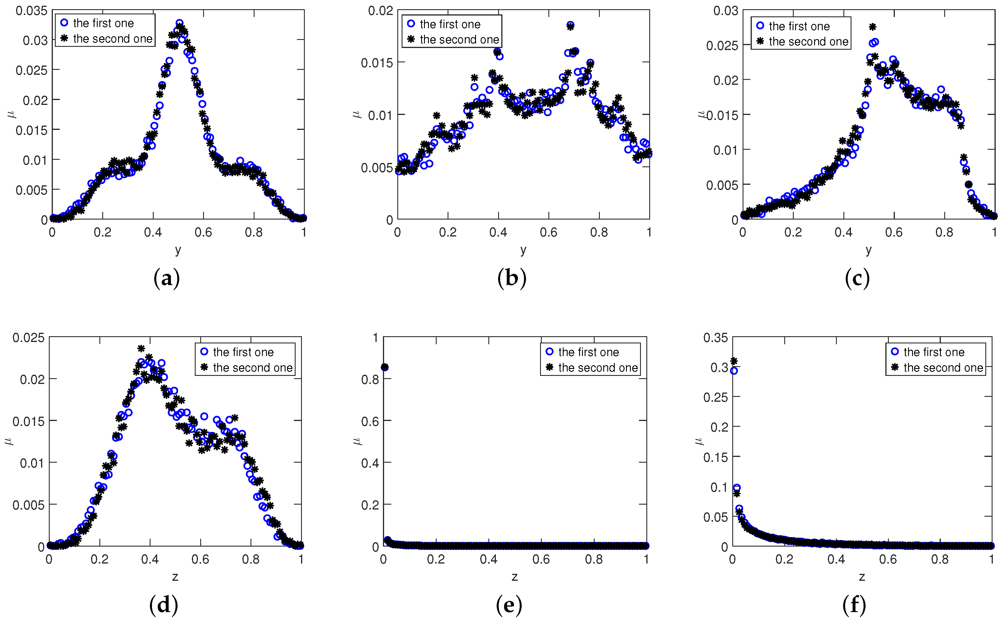
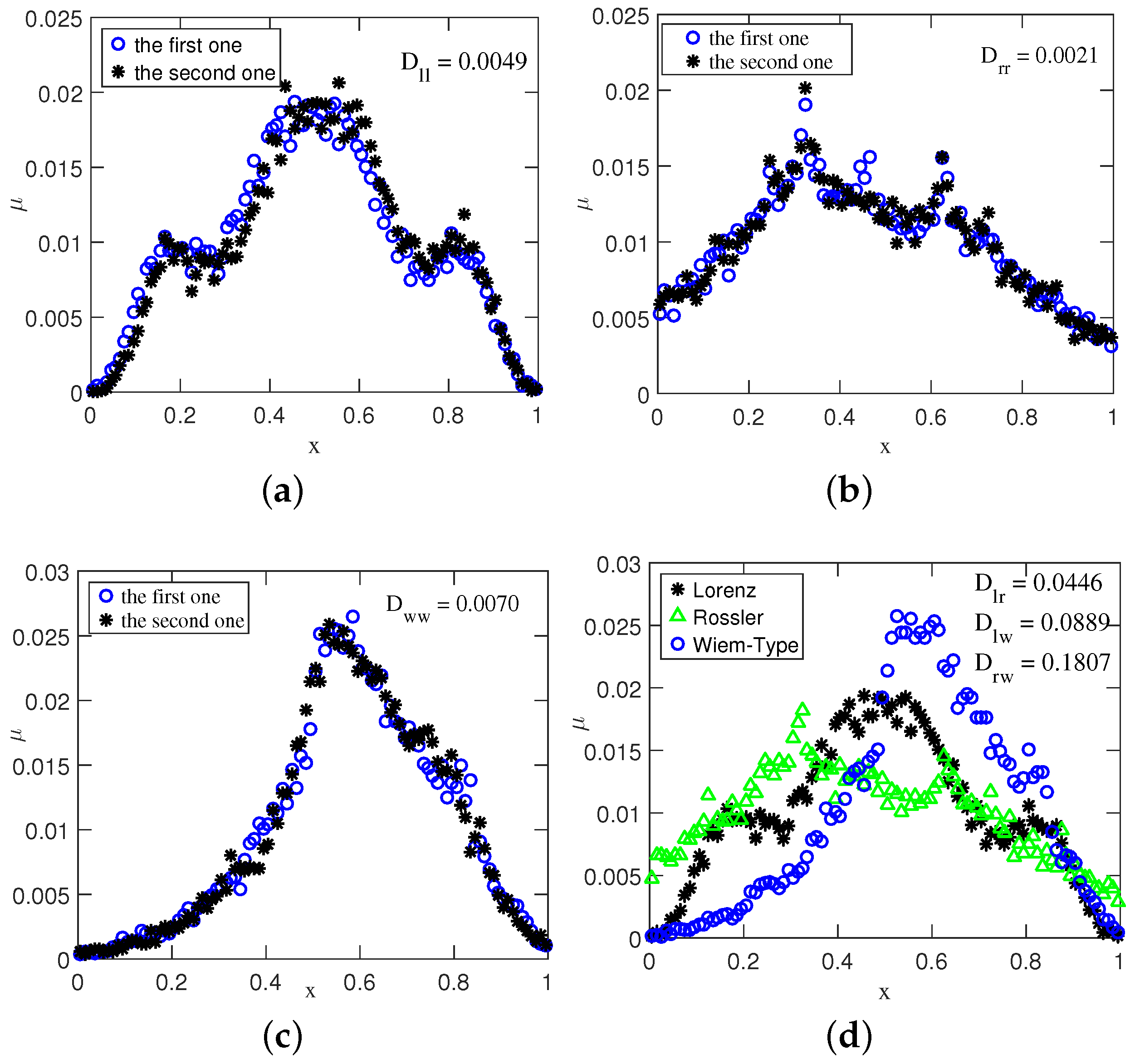
In this letter, the x-coordinates of the above systems are used. The histograms of the Lorenz series from different typical initial conditions [23] are made, and two of them that are randomly selected are shown in Figure 1a. There are 20,000 data points being used, and the length of inter-cell for the histogram is 0.01.

From Figure 1a, we can easily observe that the histograms derived from different x-coordinates (i.e., the orbits from different typical initial conditions) of the Lorenz system are almost the same. It should be noted that similar results are also obtained for the Rössler and Wiem-Type system, as shown in Figure 1b,c, respectively.

On the other hand, in Figure 1d we plot the histograms obtained from the x-coordinates of the Lorenz, Rössler, and Wiem-Type system, respectively. It can be easily seen from Figure 1d that the histograms obtained from the one-dimensional component of different systems are quite diverse. Although the difference can be perceived by human eyes, it can be better detected statistically. In the present work, the well-known Kullback–Leibler divergence (KLD) [24] is used to detect this difference, and here we are interested in the discrete type of the KLD. Generally speaking, given two discrete distributions ${\mu }_P$ and ${\mu }_Q$ with domain $\mathcal{X}$, the KLD $D_{KLD}\left(\left.{\mu }_P\right|{\mu }_Q\right)$ is defined as follows:

$$D_{KLD}\left(\left.{\mu }_P\right|{\mu }_Q\right)=\sum _{x\in \mathcal{X}}{\mu }_P\left(x\right)log\frac{{\mu }_P\left(x\right)}{{\mu }_Q\left(x\right)}.$$

(9)

The KLD is null if and only if ${\mu }_P={\mu }_Q$, and positive otherwise. In information theory, the KLD is also called the relative entropy and is widely used to measure the distance (similarity) between two distributions [25]. The KLD is also widely used in biological systems [26]. The KLD obtained from different natural measures is always larger than zero due to the finite data length. Nevertheless, a relatively small KLD means that the two natural measures are almost the same. It should be noted that two distributions ${\mu }_P$ and ${\mu }_Q$ may not have the same supports (i.e., if ${\mu }_Q\left(m\right)=0,{\mu }_P\left(m\right)\ne 0$, or ${\mu }_P\left(m\right)=0,{\mu }_Q\left(m\right)\ne 0$ for some value m). As a common procedure [27], we introduce a bias of order $\mathcal{O}\left(1/\phantom{1N^2}{N}^2\right)$, where N is the length of the signal. More precisely, the vanishing frequencies are replaced with $1/\phantom{1N}N$, and the new frequency histogram is normalized appropriately. Given two natural measures ${\mu }_P=\left[{\mu }_{P,1},{\mu }_{P,2},\cdots ,{\mu }_{P,L}\right]$ and ${\mu }_Q=\left[{\mu }_{Q,1},{\mu }_{Q,2},\cdots ,{\mu }_{Q,L}\right]$, according to the evaluation of the natural measure, ${\mu }_P$ and ${\mu }_Q$ are both defined on $[0,1]$, ${\mu }_{X,i},X\in \left\{P,Q\right\},i=1,2,\cdots ,L$ is the probability where the data fall into the interval $\left(\left(i-1\right)\Delta ,i\Delta \right)$. The calculation of the KLD $D_{KLD}\left(\left.{\mu }_P\right|{\mu }_Q\right)$ can be implemented as follows:

• Step 1: Processing the vanishing frequencies:

  $${\tilde{\mu }}_{P,i}=\left\{\begin{array}{cc}{\mu }_{P,i},& {\mu }_{P,i}\ne 0\\ 1/\phantom{1N,}N,& {\mu }_{P,i}=0\end{array}\right.$$

  (10)

  $${\tilde{\mu }}_{Q,i}=\left\{\begin{array}{cc}{\mu }_{Q,i},& {\mu }_{Q,i}\ne 0\\ 1/\phantom{1N,}N,& {\mu }_{Q,i}=0\end{array}\right.$$

  (11)

  where $N=max\left(N_P,N_Q\right)$ with $N_P$ and $N_Q$ being the length of data P and data Q, respectively.
• Step 2: Normalizing ${\tilde{\mu }}_P$ and ${\tilde{\mu }}_Q$:

  $${\tilde{\mu }}_{P,i}={\tilde{\mu }}_{P,i}/\sum _{i=1}^L{\tilde{\mu }}_{P,i}$$

  (12)

  $${\tilde{\mu }}_{Q,i}={\tilde{\mu }}_{Q,i}/\sum _{i=1}^L{\tilde{\mu }}_{Q,i}$$

  (13)
• Step 3: Calculating the $D_{KLD}\left(\left.{\tilde{\mu }}_P\right|{\tilde{\mu }}_Q\right)$:

  $$D_{KLD}\left(\left.{\tilde{\mu }}_P\right|{\tilde{\mu }}_Q\right)=\sum _{\mathrm{i}=1}^L{\tilde{\mu }}_{P,i}log\frac{{\tilde{\mu }}_{P,i}}{{\tilde{\mu }}_{Q,i}}.$$

  (14)

In order to verify the results in Figure 1, we have computed the KLDs between different chaotic systems, the average values which are carried out with 1000 Monte-Carlo experiments are shown in

Table 1. The average Kullback–Leibler divergences (KLDs) between different chaotic systems.

	Lorenz	Rössler	Wiem-Type
Lorenz	0.0049	0.0446	0.0889
Rössler	0.0731	0.0021	0.1807
Wiem-Type	0.0759	0.1247	0.0070

. In addition, the $D_{ll}$ shown in Figure 1a is the average KLD between the histograms obtained from two orbits of the Lorenz system, $D_{rr}$ in Figure 1b and $D_{ww}$ in Figure 1c are similar with $D_{ll}$. $D_{lr}$ shown in Figure 1d is the average KLD between the histograms obtained from the orbits of the Lorenz and Rössler system, $D_{lw}$ and $D_{rw}$ are similar with $D_{lr}$.

It can be seen from Table 1 that the values of KLD between different histograms of the same system are quite small, which means that they are almost the same. On the other hand, the values of KLD between the histograms of the diverse systems are relatively large, which means that they are quite different. In Figure 2 we also plot the natural measures obtained from the y and z-coordinates of these systems. From Figure 2 we can easily observe that for each system, the histograms derived from y-coordinates (or z-coordinates) with different initial values are almost the same, which means that the natural measure obtained from the y-coordinate (or z-coordinate) exists. It should be pointed out that for Rössler and Wiem-Type systems, the corresponding histograms derived from the z-coordinates are quite different from those of the y-coordinates and the x-coordinates, which means that the natural measures obtained from different components are not the same—even for the same chaotic system.

The natural invariant density and the natural measure are usually defined on the one-dimensional chaotic maps. In this letter, we extend these concepts to the chaotic systems, and find that even for the same chaotic system, the natural measures derived from different coordinates are quite different. Nevertheless, the natural measure exists for any coordinates of a chaotic system, and can be used as an RF fingerprint since they are different for diverse systems.

From the results shown in Figure 1 and Figure 2 and Table 1, we find that the natural measures of the one-dimensional component of higher dimensional systems exists, and the KLD between these natural measures can be exploited to classify the unique transmitter. In what follows we will exploit the natural measure obtained from the real data as the RF fingerprint to classify the unique transmitter. An obvious advantage of the natural measure is that the amount of data one needs can naturally increase because the natural measure will not change if one puts different orbits together, which makes the proposed method very effective—even in the case of a relatively small amount of data.

3. Results

The aim of this letter is to extract a valid RF fingerprint from the given signal and implement an effective recognition. We will check the performance of the proposed method by utilizing the data obtained from real applications. The data are derived from the Automatic Identification System (AIS) signals emitted from ships. The center frequency of AIS burst signal is 161.975 MHz or 162.025 MHz. The data bits are modulated with Gaussian Minimum Shift Keying (GMSK) with a bandwidth of 25 KHz, and the data rate is 9600 bits per second. The signals are collected by an antenna and a signal monitoring system located near a port in China. The interest signal is down-converted and digitized with an analog-to-digital converter. The signal-to-noise ratio (SNR) for all data samples is about 18 dB, and the oversampling rate is 40.

In the experiment, we have four different transmitters that are produced by four diverse manufacturers, which means that measure sets come from different emitter types and the process of their recognition is based only on type classification. In other words, we have four classes of data, which are denoted as ${\mathrm{T}}_i,i=1,2,3,4$, and there are 40 bursts in each class. After obtaining the data, we then extract the transient part of each burst by using a method similar to that in [28] and normalize these transients to $[0,1]$. Since the number of bursts is small and the transient part of each burst is very short (about 0.83 milliseconds), we will do the experiment just as the sampling with replacement. In each run, the experiment is implemented as follows:

• Step 1: Randomly choosing three normalized transients from each class and serially connecting them to form a big transient. This big transient will be regarded as the testing data;
• Step 2: Serially connecting the remaining normalized transients in each class to form another big transient and regarding it as the training data;
• Step 3: Calculating the corresponding natural measures; i.e., four natural measures for the testing data, denoted as ${\mu }_t,t=1,2,3,4$, and four natural measures for the training data, denoted as ${\mu }_i,i=1,2,3,4$;
• Step 4: Calculating the KLD between ${\mu }_t$ and ${\mu }_i$, $D_{KLD}\left({\mu }_i\left|{\mu }_t\right.\right),i=1,2,3,4;t=1,2,3,4$;
• Step 5: Identifying each testing data; i.e., finding the smallest $D_{KLD}\left({\mu }_i\left|{\mu }_t\right.\right),i=1,2,3,4$ for a given t. For example, if $D_{KLD}\left({\mu }_4\left|{\mu }_t\right.\right)$ is the smallest when $t=1$, then the first testing data belong to the fourth class.

In each run, after the above steps, the testing data will be put back to the corresponding data sets and the above steps will be repeated until 100 runs are completed. The classification confusion matrix obtained from 100 trials is shown in

Table 2. Classification confusion matrix for four transmitters.

	T1	T2	T3	T4
T1	100%	0	0	0
T2	0	99%	0	1%
T3	0	0	100%	0
T4	2%	0	0	98%

.

We can observe from Table 2 that above 98% identification accuracy is achieved for all the emitters, which means that the proposed method can classify these transmitters successfully. It is important to point out that there are only 320 data points in the transient part of each burst, which means that the amount of data in each trial is very small. The results shown in Table 2 demonstrate that the proposed method based on the natural measure is very effective for SEI, even though the amount of data is quite small and the sample rate is low.

The SEI method based on the normalized permutation entropy (NPE) [20] is similar to the proposed method. Hence, the NPE-based SEI method is used as a gold standard in this letter. In order to make a comparison between the NPE-based method and the proposed method, the classification confusion matrix of the NPE-based method is calculated and the results are shown in

Table 3. Classification confusion matrix of the normalized permutation entropy (NPE)-based method for four transmitters.

	T1	T2	T3	T4
T1	70%	2.5%	0	27.5%
T2	5%	95%	0	0
T3	0	0	95%	5%
T4	55%	0	2.5%	42.5%

. It should be noted that 40 Monte Carlo runs are implemented for each transmitter since there are only 40 bursts in each class. In this experiment, a k-nearest neighbor discriminatory classifier [29] with $k=4$ is employed. To derive the NPE, the transient part of each burst is used and the embedding dimension D is set to three, since the transient is quite short. As can be seen from Table 3, the NPE-based method achieves high classification accuracy for T2 and T3, it achieves low classification accuracy for T1, and classifies T4 incorrectly. From Table 3 we can also observe that T4 can be easily recognized as T1 and vice versa. The parameters of the amplifiers in these transmitters may be very close, which will lead to the similar permutations [20]. However, the proposed method is not affected by this, and it still identifies T4 and T1 correctly. Comparing Table 2 and Table 3, it can be easily observed that the performance of the proposed method is better than that of the NPE-based method.

In practice, the time consumption of a method is also an important consideration. In order to check the time consumption of the proposed method, the average time consumption via 160 Monte Carlo runs (40 runs for each class) of the NPE-based method and the proposed method for different data lengths are shown in

Table 4. Time consumptions of the NPE-based method and the proposed method with different data lengths (unit: s).

	N = 320	N = 1280
NPE-based	0.0031	0.0035
the proposed	0.0014	0.0032

. The embedding dimensions of the NPE-based method for the two data lengths are 3 and 5, respectively. It can be seen from Table 4 that the time consumptions of the proposed method are smaller than those of the NPE-based method—at least in the case of a small amount of data. The experiments are run on a computer with a 3.40 GHz Intel Core i7-2600K CPU and 8.00 GB RAM. The release of MATLAB is 2016b.

4. Conclusions and Future Directions

In summary, a novel SEI method based on the natural measure of the one-dimensional component of chaotic systems is proposed in this letter. We first verify that the natural measure of the one-dimensional component of higher dimensional chaotic system exists and they are quite different for diverse systems. Next, the natural measure is used as an RF fingerprint to classify different emitters once these emitters are regarded as nonlinear systems. Then, we put different transient parts of the bursts obtained from the same emitters together in order to increase the amount of data in consideration of the property of the natural measure. Finally, the KLD is exploited to quantify the distance between different natural measures and classify diverse transmitters. The data from real application are used to test the validity of the proposed method. The experimental results show that the proposed method is not only easy to operate, but also very effective for SEI even though the amount of data is small and the sample rate is low in real application. Moreover, we will investigate the application of the proposed method to sensor networks in the future, just as the detection of target [30] and the modulation classification [31] have been extended to this field.

References

- Li, L.; Ji, H. Radar emitter recognition based on cyclostationary signatures and sequential iterative least-square estimation. Expert Syst. Appl. 2011, 38, 2140–2147. [Google Scholar] [CrossRef]
- Ciuonzo, D.; Rossi, P.S. Distributed detection of a non-cooperative target via generalized locally-optimum approaches. Inf. Fusion 2017, 36, 261–274. [Google Scholar] [CrossRef]
- Dulek, B.; Ozdemir, O.; Varshney, P.K.; Su, W. Distributed maximum likelihood classification of linear modulations over nonidentical flat block-fading Gaussian channels. IEEE Trans. Wirel. Commun. 2015, 14, 724–737. [Google Scholar] [CrossRef]
- Talbot, K.I.; Duley, P.R.; Hyatt, M.H. Specific emitter identification and verification. Technol. Rev. 2003, 1, 113–133. [Google Scholar]
- Suski, W.C., II; Temple, M.A.; Mendenhall, M.J.; Mills, R.F. Radio frequency fingerprinting commercial communication devices to enhance electronic security. Int. J. Electron. Secur. Digit. Forensics 2008, 1, 301–322. [Google Scholar]
- Cobb, W.E.; Laspe, E.D.; Baldwin, R.O.; Temple, M.A.; Kim, Y.C. Intrinsic physical-layer authentication of integrated circuits. IEEE Trans. Inf. Forensics Secur. 2012, 7, 14–24. [Google Scholar] [CrossRef]
- Kawalec, A.; Owczarek, R. Radar emitter recognition using intrapulse data. In Proceedings of the International Conference on Microwaves, Radar and Wireless Communications, Warsaw, Poland, 17–19 May 2004; pp. 435–438.
- Dudczyk, J.; Kawalec, A.; Owczarek, R. An application of iterated function system attractor for specific radar source identification. In Proceedings of the International Conference on Microwaves, Radar and Wireless Communications, Wroclaw, Poland, 19–21 May 2008; pp. 1–4.
- Dudczyk, J.; Kawalec, A. Identification of emitter sources in the aspect of their fractal features. Bull. Pol. Acad. Sci. Tech. Sci. 2013, 61, 2013–2065. [Google Scholar] [CrossRef]
- Dudczyk, J.; Kawalec, A. Specific emitter identification based on graphical representation of the distribution of radar signal parameters. Bull. Pol. Acad. Sci. Tech. Sci. 2015, 63, 391–396. [Google Scholar] [CrossRef]
- Dudczyk, J. Radar Emission Sources Identification Based on Hierarchical Agglomerative Clustering for Large Data Sets. J. Sens. 2016, 2016, 1879327. [Google Scholar] [CrossRef]
- Yang, Z.; Wei, Q.; Sun, H.; Arumugam, N. Robust Radar Emitter Recognition Based on the Three-Dimensional Distribution Feature and Transfer Learning. Sensors 2016, 16, 289. [Google Scholar] [CrossRef] [PubMed] [Green Version]
- Danev, B.; Capkun, S. Transient-based identification of wireless sensor nodes. In Proceedings of the 2009 International Conference on Information Processing in Sensor Networks, San Francisco, CA, USA, 13–16 April 2009; pp. 25–36.
- Klein, R.; Temple, M.A.; Mendenhall, M.J.; Reising, D.R. Sensitivity analysis of burst detection and RF fingerprinting classification performance. In Proceedings of the 2009 IEEE International Conference on Communications, Dresden, Germany, 14–18 June 2009; pp. 1–5.
- Danev, B.; Capkun, S. Physical-Layer Identification of Wireless Sensor Nodes. Available online: http://e-collection.library.ethz.ch/eserv/eth:4995/eth-4995-01.pdf (accessed on 10 March 2017).
- Brik, V.; Banerjee, S.; Gruteser, M.; Oh, S. Wireless device identification with radiometric signatures. In Proceedings of the 14th ACM International Conference on Mobile Computing and Networking, San Francisco, CA, USA, 14–19 September 2008; pp. 116–127.
- Scanlon, P.; Kennedy, I.O.; Liu, Y. Feature extraction approaches to RF fingerprinting for device identification in femtocells. Bell Labs Tech. J. 2010, 15, 141–151. [Google Scholar]
- Bertoncini, C.; Rudd, K.; Nousain, B.; Hinders, M. Wavelet fingerprinting of radio-frequency identification (RFID) tags. IEEE Trans. Ind. Electron. 2012, 59, 4843–4850. [Google Scholar] [CrossRef]
- Carroll, T. A nonlinear dynamics method for signal identification. Chaos Interdiscip. J. Nonlinear Sci. 2007, 17, 023109. [Google Scholar] [CrossRef] [PubMed]
- Huang, G.; Yuan, Y.; Wang, X.; Huang, Z. Specific Emitter Identification Based on Nonlinear Dynamical Characteristics. Can. J. Electr. Comput. Eng. 2016, 39, 34–41. [Google Scholar] [CrossRef]
- Polak, A.C.; Dolatshahi, S.; Goeckel, D.L. Identifying wireless users via transmitter imperfections. IEEE J. Sel. Areas Commun. 2011, 29, 1469–1479. [Google Scholar] [CrossRef]
- Zhang, J.; Wang, F.; Dobre, O.A.; Zhong, Z. Specific Emitter Identification via Hilbert-Huang Transform in Single-Hop and Relaying Scenarios. IEEE Trans. Inf. Forensics Secur. 2016, 11, 1192–1205. [Google Scholar] [CrossRef]
- Ott, E. Chaos in Dynamical Systems; Cambridge University Press: Cambridge, UK, 2002; pp. 1–56. [Google Scholar]
- Cachin, C. An information-theoretic model for steganography. Inf. Comput. 2004, 192, 41–56. [Google Scholar] [CrossRef]
- Cheng, Y.; Hua, X.; Wang, H.; Qin, Y.; Li, X. The Geometry of Signal Detection with Applications to Radar Signal Processing. Entropy 2016, 18, 381. [Google Scholar] [CrossRef]
- Baez, J.C.; Pollard, B.S. Relative entropy in biological systems. Entropy 2016, 18, 46. [Google Scholar] [CrossRef]
- Roldán, É.; Parrondo, J.M. Entropy production and Kullback-Leibler divergence between stationary trajectories of discrete systems. Phys. Rev. E 2012, 85, 031129. [Google Scholar] [CrossRef] [PubMed]
- Yuan, H.; Hu, A. Preamble-based detection of Wi-Fi transmitter RF fingerprints. Electron. Lett. 2010, 46, 1165–1167. [Google Scholar] [CrossRef]
- Danev, B.; Luecken, H.; Capkun, S.; El Defrawy, K. Attacks on physical-layer identification. In Proceedings of the Third ACM Conference on Wireless Network Security, Hoboken, NJ, USA, 22–24 March 2010; pp. 89–98.
- Ciuonzo, D.; Papa, G.; Romano, G.; Rossi, P.S.; Willett, P. One-bit decentralized detection with a Rao test for multisensor fusion. IEEE Signal Process. Lett. 2013, 20, 861–864. [Google Scholar] [CrossRef]
- Su, W. Modulation Classification of Single-Input Multiple-Output Signals using Asynchronous Sensors. IEEE Sens. J. 2015, 15, 346–357. [Google Scholar] [CrossRef]
Figure 1.
The histograms obtained from two arbitrary (a) Lorenz; (b) Rösser; and (c) Wiem-Type time series (the x-coordinate); (d) The histograms obtained from the x-coordinates of the Lorenz, Rössler, and Wiem-Type system.
Figure 2.
The histograms obtained from two arbitrary (a) Lorenz; (b) Rösser; and (c) Wiem-Type time series (the y-coordinate). The histograms obtained from two arbitrary (d) Lorenz; (e) Rösser; and (f) Wiem-Type time series (the z-coordinate).