Thermoeconomic Optimization of an Irreversible Novikov Plant Model under Different Regimes of Performance

Abstract

The so-called Novikov power plant model has been widely used to represent some actual power plants, such as nuclear electric power generators. In the present work, a thermo-economic study of a Novikov power plant model is presented under three different regimes of performance: maximum power (MP), maximum ecological function (ME) and maximum efficient power (EP). In this study, different heat transfer laws are used: The Newton’s law of cooling, the Stefan–Boltzmann radiation law, the Dulong–Petit’s law and another phenomenological heat transfer law. For the thermoeconomic optimization of power plant models, a benefit function defined as the quotient of an objective function and the total economical costs is commonly employed. Usually, the total costs take into account two contributions: a cost related to the investment and another stemming from the fuel consumption. In this work, a new cost associated to the maintenance of the power plant is also considered. With these new total costs, it is shown that under the maximum ecological function regime the plant improves its economic and energetic performance in comparison with the other two regimes. The methodology used in this paper is within the context of finite-time thermodynamics.

1. Introduction

During more than four decades, a branch of irreversible thermodynamics called finite-time thermodynamics (FTT) has been developed [1,2,3,4,5]. Within the context of FTT, it has been possible to elaborate detailed models of heat engines working at finite-time and with entropy production [6,7,8,9,10]. One of the applications of FTT has been in the field of thermoeconomics [11,12,13,14]. In 1995, Alexis De Vos introduced for the first time a thermoeconomic study for the Novikov plant model [15]. In his study, De Vos takes into account two costs: a cost related to the investment and another cost associated to the fuel consumption. From his thermoeconomic study, De Vos found that the optimal thermoeconomic efficiency under maximum power conditions is between the Curzon–Ahlborn (CA) efficiency and Carnot efficiency [16]. Here, De Vos refers to the power production rate $W$ of the Novikov plant model. Later, Barranco-Jiménez and Angulo-Brown [17,18] extended the De Vos thermoeconomic approach, but using the so-called ecological function [19,20], and they also showed that the economical efficiency under this regime of performance lies between the CA efficiency and the Carnot efficiency. In 2009, Barranco-Jiménez [21] studied the thermoeconomics of a nonendoreversible Novikov engine. He used different heat transfer laws: The Newton’s law of cooling, the Stefan–Boltzmann radiation law [22], the Dulong–Petit’s law of cooling [23] and a phenomenological heat transfer law [24,25] (the usage of each transfer law depends on the kind of heat engine model to describe [22,23,24,25,26,27]). He calculated the thermoeconomic optimal efficiencies under two regimes of performance, namely, the maximum power regime and the ecological regime, and he found that when the Novikov model maximizes the ecological function, it reduces the rejected heat to the environment down to about 50% with respect to the heat rejected under maximum power conditions. Recently, Pacheco-Paez et al. 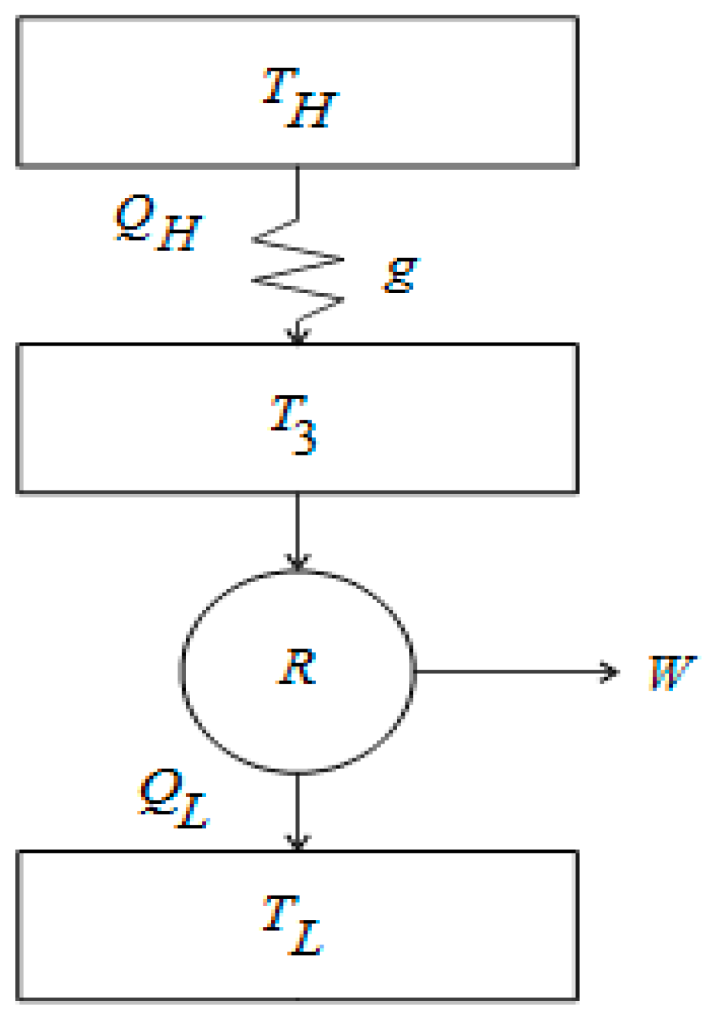[28,29] made a thermoeconomic analysis of a Novikov plant following the De Vos approach (with a linear heat transfer law) but including a new cost associated to the maintenance of the power plant. The aim of this paper is to extend the thermoeconomic analysis of the Novikov plant model (see Figure 1) by considering different heat transfer laws. Besides, in the optimization of the benefit functions, we take into account a new cost associated to the maintenance of the power plant [28,29]. In our study, we also consider three regimes of performance: maximum power (MP) [3], maximum efficient power (EP) [30,31] and maximum ecological function (ME) [19,20]. The methodology used in this paper is within the context of finite-time thermodynamics. Apart from the De Vos method, there exist other approaches for the thermoeconomic analysis of power plant models. Interestingly, the thermoeconomic analysis based on exergy has played an important role in this discipline [32,33,34,35,36]. The work is organized as follows: In Section 2, we present the thermoeconomic analysis of the Novikov power plant under different criteria of performance. In Section 3, we analyze the environmental impact of the thermoeconomic model, and finally in Section 4, we present our conclusions.

2. Thermoeconomic Analysis

Applying the first law of thermodynamics to Figure 1, the power output is given by,

$$W=Q_H-Q_L,$$

(1)

where $Q_H$ and $Q_L$ are the heat transfers between the thermal baths and the working fluid ($W$, $Q_H$ and $Q_L$ are quantities per cycle’s period). On the other hand, the internal efficiency of the engine is given by [21],

$$\eta =\frac{W}{Q_H}=1-\frac{\tau }{R}\frac{1}{\theta },$$

(2)

where $\tau =T_L/T_H$, $\theta =T_3/T_H$ and the parameter $R=\mathrm{∆}{S}_1/\left|\mathrm{∆}{S}_2\right|$ is the non-endoreversibility parameter [37,38] (which characterizes the degree of internal irreversibility that comes from the Clausius inequality), $\mathrm{∆}{S}_1$ being the change of the internal entropy along the hot isothermal branch and $\mathrm{∆}{S}_2$ the entropy change corresponding to the cold isothermal compression. This parameter in principle is within the interval $0<R\le 1$ ($R=1$ for the endoreversible limit). If we consider that the heat transferred between the hot source and the working fluid obeys a generalized law of the type,

$$Q_H=g{T_H}^n{\left(1-\theta \right)}^n,$$

(3)

where the exponent $n$ can be any real number different from zero and it takes the values $n=1$ for a Newtonian heat transfer law (N) and $n=5/4$ for a Dulong–Petit heat transfer law (DP) [23,27] and $g$ is the thermal conductance (see Figure 1). From Equations (2) and (3), the power output $\left(W=\eta Q_H\right)$ results in

$$W=g{T}_H^n\eta {\left(1-\frac{\tau }{R(1-\eta )}\right)}^n$$

(4)

The De Vos thermoeconomical analysis considers a profit function $F$, which is maximized [11]. This profit function is given by the quotient of the power output $W$ (that is, the power production rate $W$ of the Novikov plant model) and the total costs involved in the performance of the power plant, that is

$$F=\frac{W}{C}$$

(5)

Apart from this De Vos method, there exist other approaches for the thermoeconomic analysis of power plant models. Significantly, the thermoeconomic analysis based on exergy has played an important role in this matter [32,33,34,35,36]. In his study, De Vos assumed that the running costs of the plant consist of two parts: a capital cost which is proportional to the investment and, therefore, to the size of the plant, and a fuel cost that is proportional to the fuel consumption and, therefore, to the heat input rate. In this work, we also take into account a cost associated to the maintenance of the power plant which is taken as proportional to the power output of the plant. This choice is based on an intuitive idea that has to do with the wheatering of the engine depending on its excessive usage. Therefore, the running costs of the plant exploitation are now defined as,

$$C=a{Q}_{\max }+b{Q}_H+cW,$$

(6)

where the proportionality constants a, b and c have units of $/Watt, and $Q_{\max }=g{T_H}^n{\left(1-\tau \right)}^n$ is the maximum heat that can be extracted from the heat reservoir without supplying work in the same manner previously considered by De Vos [11] (see Figure 1). Equation (6) is taken as a linear relation inspired in the linear character of the first law of thermodynamics [39]. Using Equations (3) and (4), the running costs of the plant are given by,

$$C=ag{T_H}^n\left[{\left(1-\tau \right)}^n+\beta {\left(1-\frac{\tau }{R(1-\eta )}\right)}^n+\gamma \eta {\left(1-\frac{\tau }{R(1-\eta )}\right)}^n\right],$$

(7)

where $\beta =b/a$ and $\gamma =c/a$ ($0\le \beta <\infty$ and $0\le \gamma$). After substituting Equations (4) and (7) into Equation (5), the dimensionless objective profit function is given by,

$$a{F}_{MP}^{N-DP}=\frac{\eta {\left(1-\frac{\tau }{R(1-\eta )}\right)}^n}{{\left(1-\tau \right)}^n+\beta {\left(1-\frac{\tau }{R(1-\eta )}\right)}^n+\gamma \eta {\left(1-\frac{\tau }{R(1-\eta )}\right)}^n},$$

(8)

which is valid for the transfer laws of Newton ($N$), and Dulong–Petit ($DP$). Now, we define two additional objective functions, one in terms of the so-called modified ecological function ($E\equiv W-\in T_L\sigma ,$ with $\sigma$ the rate of total entropy production of the Novikov model and $\in$ a parameter which depends on the heat transfer law used in the Novikov model [19,20]). This function is a slight modification of the former ecological function [19], which preserves the original physical meaning of that function; that is, it represents a good trade-off between high power output and low dissipation. On the other hand, we also use a profit function based on the efficient power [30,31] $\left(P_{EP}\equiv \eta W\right)$, which is an objective function of the class of compromise functions looking for a good trade-off between power output and efficiency. Both objective functions are divided by the total costs involved in the performance of the plant, that is, $F_{EP}=\frac{\eta W}{C}$ and $F_{ME}=\frac{W-\in T_L\sigma }{C}$, respectively. Analogously to Equation (8), by using Equations (4), (5) and (7), $F_{EP}$ and $F_{ME}$ are given by,

$$a{F}_{EP}^{N-DP}=\frac{{\eta }^2{\left(1-\frac{\tau }{R(1-\eta )}\right)}^n}{{\left(1-\tau \right)}^n+\beta {\left(1-\frac{\tau }{R(1-\eta )}\right)}^n+\gamma \eta {\left(1-\frac{\tau }{R(1-\eta )}\right)}^n},$$

(9)

and,

$$a{F}_{ME}^{N-DP}=\frac{\left[\left(1+\epsilon \right)\eta -\epsilon (1-\tau )\right]{\left(1-\frac{\tau }{R(1-\eta )}\right)}^n}{{\left(1-\tau \right)}^n+\beta {\left(1-\frac{\tau }{R(1-\eta )}\right)}^n+\gamma \eta {\left(1-\frac{\tau }{R(1-\eta )}\right)}^n}.$$

(10)

The maximization of the objective functions given by Equations (8)–(10) by means of ${\frac{d\left(aF\right)}{d\eta }|}_{{\eta }^{\ast }}=0$ gives the corresponding optimal efficiencies. 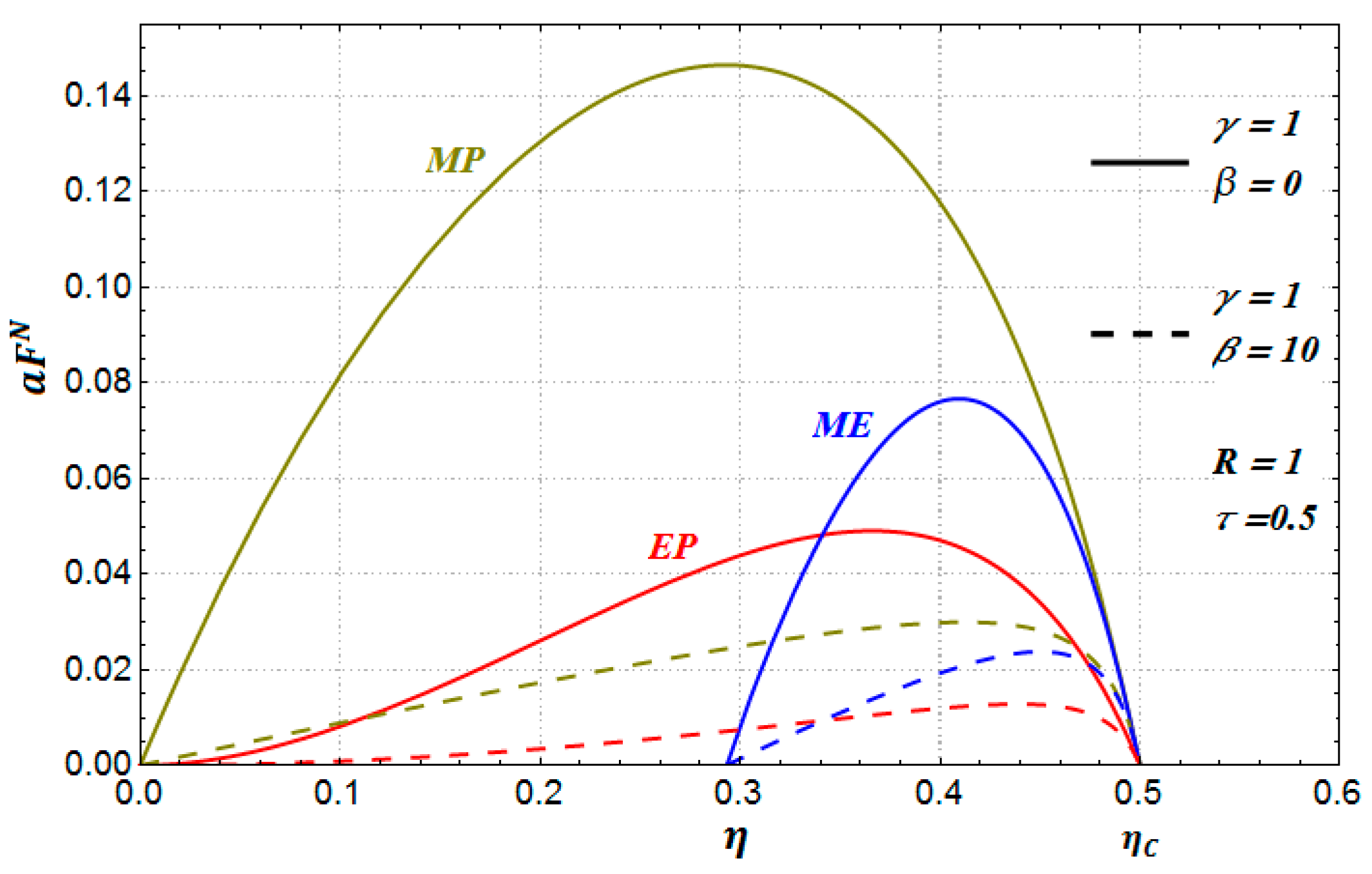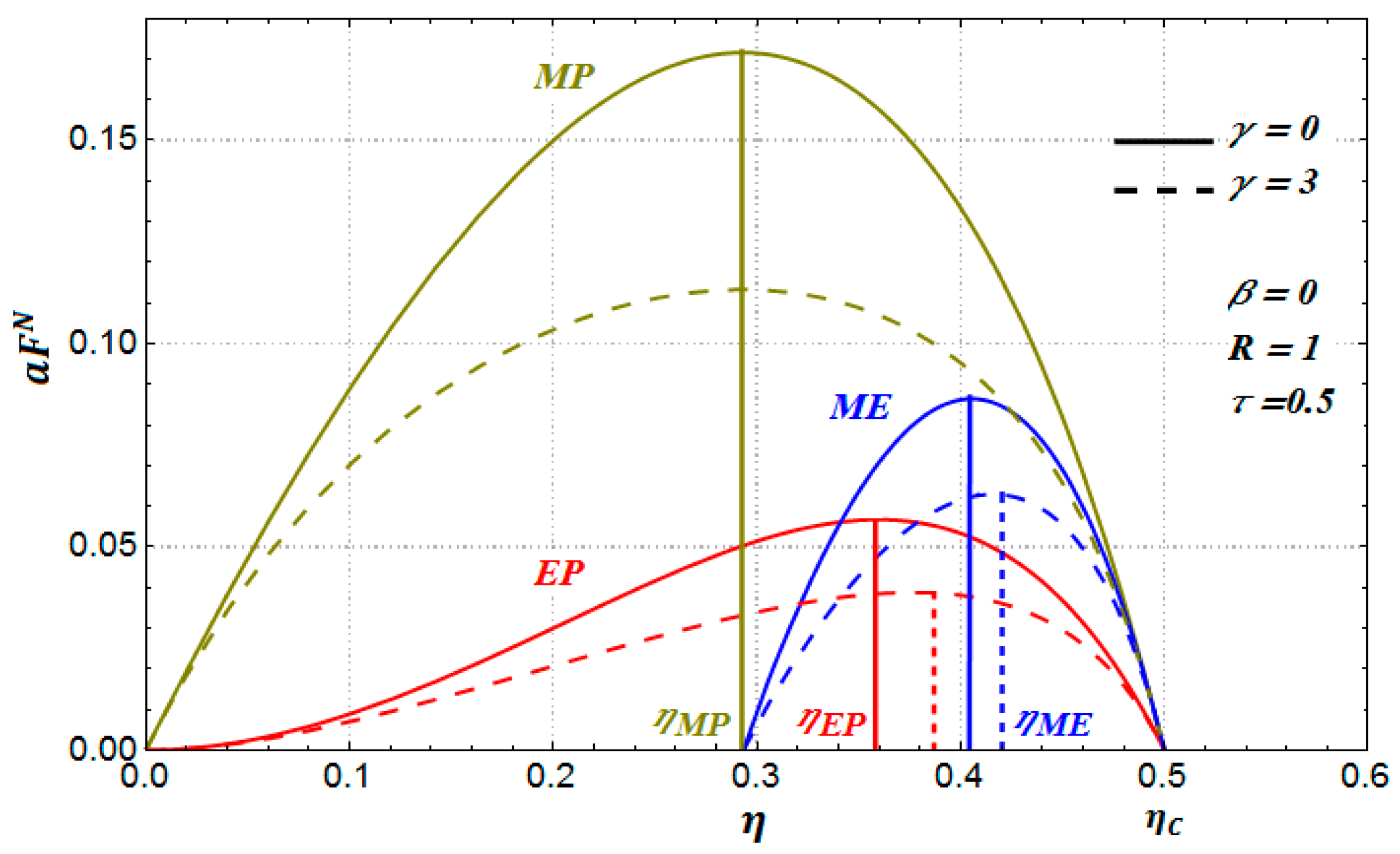Therefore, taking the derivatives of $a{F}_{MP}^{N-DP}$, $a{F}_{PE}^{N-DP}$ and $a{F}_{ME}^{N-DP}$ with respect to $\eta$ and setting them equal to zero, we obtain the optimal efficiency $\left({\eta }^{\ast }\right)$ that maximizes Equations (8)–(10), respectively. In Figure 2, for the case of a Newton heat transfer law ($n=1$ in Equation (3)), we show the behavior of the three objective functions versus the internal efficiency $\eta$ for the following arbitrary values $R=1$ (endoreversible case), $\beta =0$ and $\tau =0.5$. We observe in Figure 2 that there exists an efficiency value $\left({\eta }^{\ast }\right)$ which depends on the parameter $\gamma$. The benefits function diminishes as the parameter $\gamma$ increases. Besides, for the case of maximum power conditions, the maximum value of $a{F}^N$ is obtained for practically the same value of $\eta$ for the two values of $\gamma$ considered.

In Figure 3, we can observe for the three benefit functions how the optimal efficiency tends to the reversible value (Carnot efficiency) when $\beta \to \infty$, such as it occurs in the De Vos approach [11,21].

The optimal efficiencies are obtained in terms of the dimensionless parameter $\beta$, but this parameter is not easy to evaluate [11] and it is more convenient to work in terms of the so-called fuel fractional cost ($f$) [11,17], defined as the ratio between the fuel cost and the total costs of the plant, that is,

$$f=\frac{b{Q}_H}{a{Q}_{\max }+b{Q}_H+cW},$$

(11)

which is in the interval $0\le f<1$. From the previous equation and by using Equations (2)–(4), we get

$$\beta =\left(\frac{f}{1-f}\right)\left[\frac{{\left(1-\tau \right)}^n+\gamma \eta {\left(1-\frac{\tau }{R(1-\eta )}\right)}^n}{{\left(1-\frac{\tau }{R(1-\eta )}\right)}^n}\right].$$

(12)

From Equations (8)–(10), we can numerically find the optimal efficiencies by solving polynomial equations of the form: $H\left(\tau ,f,\gamma ,R,\eta \right)=0$. However, some analytical expressions can be obtained for $\gamma =0$ in the cases of both Newton ($n=1$) and Dulong–Petit ($n=5/4$) laws previously reported in [21]. For the case of maximum power output, the optimal efficiencies are given by [20]

$${\eta }_{MP}^N\left(\tau ,f,R\right)=1-\frac{f}{2R}\tau -\frac{\sqrt{4(1-f)R\tau +f^2{\tau }^2}}{2R}.$$

(13a)

$${\eta }_{MP}^{DP}\left(\tau ,f,R\right)=1-\frac{10\left(f-1\right)\tau }{\left(5f-1\right)\tau +\sqrt{80(1-f)R\tau +{\left(1-5f\right)}^2{\tau }^2}}.$$

(13b)

As it was previously mentioned, under the maximum power conditions, the optimum value of $\eta$ does not appreciably change the maximum of the benefit function, that is, the optimal efficiency is practically independent of the parameter $\gamma$, which is associated to the maintenance costs of the plant (see Figure 2). Interestingly, the inclusion of this new parameter has a remarkable effect on the optimal efficiencies for the cases of ME and EP maximizations. In fact, ${\eta }_{ME}^{*}$ and ${\eta }_{EP}^{*}$ increase with respect to the results without maintenance costs (see Figure 2); that is, better maintenance is reflected as better efficiency. For the case of maximum efficient power and maximum ecological function (with $\gamma =0$), the optimal efficiencies are given by,

$${\eta }_{EP}^N\left(\tau ,f,R\right)=1-\frac{\left(1+f\right)}{4R}\tau -\frac{\sqrt{8(1-f)R\tau +{\left(1+f\right)}^2{\tau }^2}}{4R},$$

(14a)

$${\eta }_{EP}^{DP}\left(\tau ,f,R\right)=1-\frac{10(f-1)\tau }{(3+5f)\tau +\sqrt{160(1-f)R\tau +{(3+5f)}^2{\tau }^2}},$$

(14b)

$${\eta }_{ME}^N\left(\tau ,f,R\right)=1-\frac{f}{2R}\tau -\frac{\sqrt{4(1-f)R{\tau }^{3/2}+f^2{\tau }^2}}{2R},$$

(15a)

$${\eta }_{ME}^{DP}\left(\tau ,f,R\right)=1-\frac{100(1-f)\tau }{(1-5f)\mathsf{\Lambda }+\sqrt{800\mathsf{\Lambda }(1-f)R+{\left[(1-5f)\mathsf{\Lambda }\right]}^2}}.$$

(15b)

where $\mathsf{\Lambda }=\tau +\sqrt{\tau (80+\tau )}$. For the cases $f=0$ and $R=1$, from Equations (13a), (14a) and (15a), we obtain the optimal efficiencies ${\eta }_{CA}=1-{\tau }^{1/2}$, ${\eta }_{EP}=1-\frac{\tau }{4}-\frac{{\left[8\tau (1+\tau )\right]}^{1/2}}{4}$ and ${\eta }_{ME}=1-{\tau }^{3/4}$ previously reported by Curzon-Ahlborn [16], Yilmaz [30] and Arias-Hernández and Angulo-Brown [20], for the Curzon-Ahlborn heat engine under maximum power output, maximum efficient power and maximum ecological function conditions, respectively.

Now, we consider two other heat transfer laws between the hot source and the working fluid as follows,

$$Q_H=g{T_H}^n\left(1-{\theta }^n\right)Sign(n),$$

(16)

$$Q_{\max }=g{T_H}^n\left(1-{\tau }^n\right)Sign(n),$$

(17)

Here, the exponent $n$ takes the values of $n=-1$ for a phenomenological heat transfer law ($Ph$) [24,25] and $n=4$ for a Stefan–Boltzmann (SB) radiation law ([22,26]) and the Sign function leads to $Sign(n)=1$ if $n>0$, and $Sign(n)=-1$ if $n<0$. In this case, the objective functions under the three regimes considered result in,

$$a{F}_{MP}^{SB-Ph}=\frac{\eta \left[1-{\left(\frac{\tau }{R(1-\eta )}\right)}^n\right]}{\left(1-{\tau }^n\right)+\beta \left[1-{\left(\frac{\tau }{R(1-\eta )}\right)}^n\right]+\gamma \eta \left[1-{\left(\frac{\tau }{R(1-\eta )}\right)}^n\right]},$$

(18)

$$a{F}_{EP}^{SB-Ph}=\frac{{\eta }^2\left[1-{\left(\frac{\tau }{R(1-\eta )}\right)}^n\right]}{\left(1-{\tau }^n\right)+\beta \left[1-{\left(\frac{\tau }{R(1-\eta )}\right)}^n\right]+\gamma \eta \left[1-{\left(\frac{\tau }{R(1-\eta )}\right)}^n\right]},$$

(19)

and,

$$a{F}_{ME}^{SB-Ph}=\frac{\left[2\eta -(1-\tau )\right]\left[1-{\left(\frac{\tau }{R(1-\eta )}\right)}^n\right]}{\left(1-{\tau }^n\right)+\beta \left[1-{\left(\frac{\tau }{R(1-\eta )}\right)}^n\right]+\gamma \eta \left[1-{\left(\frac{\tau }{R(1-\eta )}\right)}^n\right]}.$$

(20)

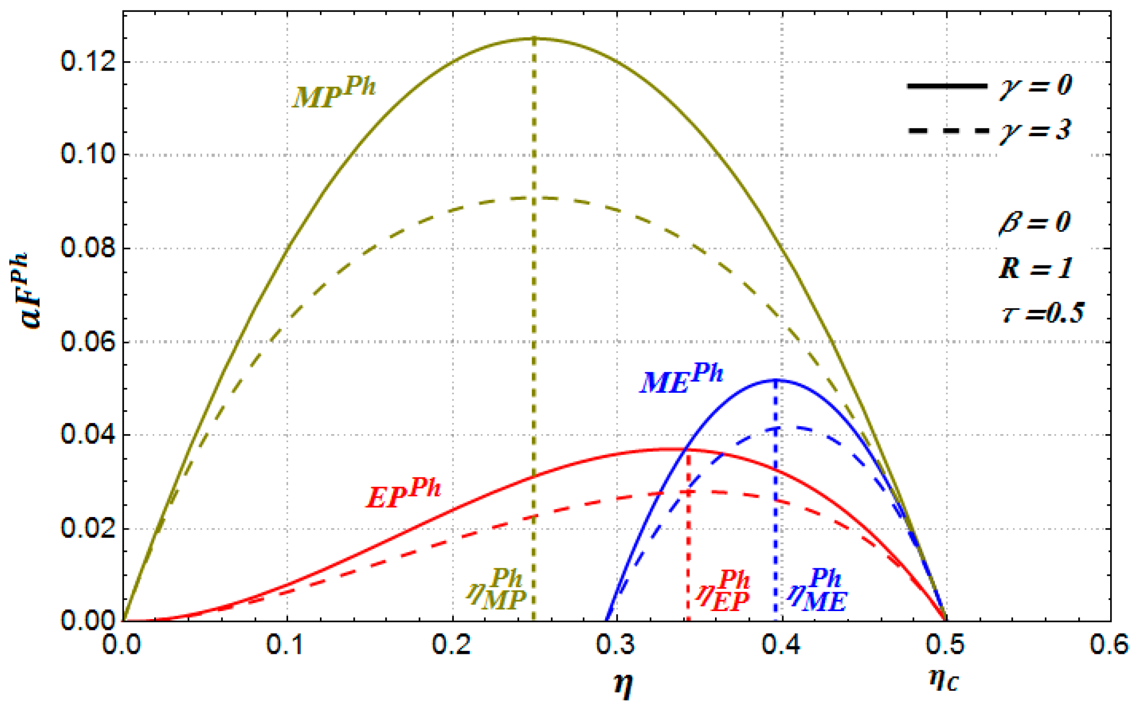
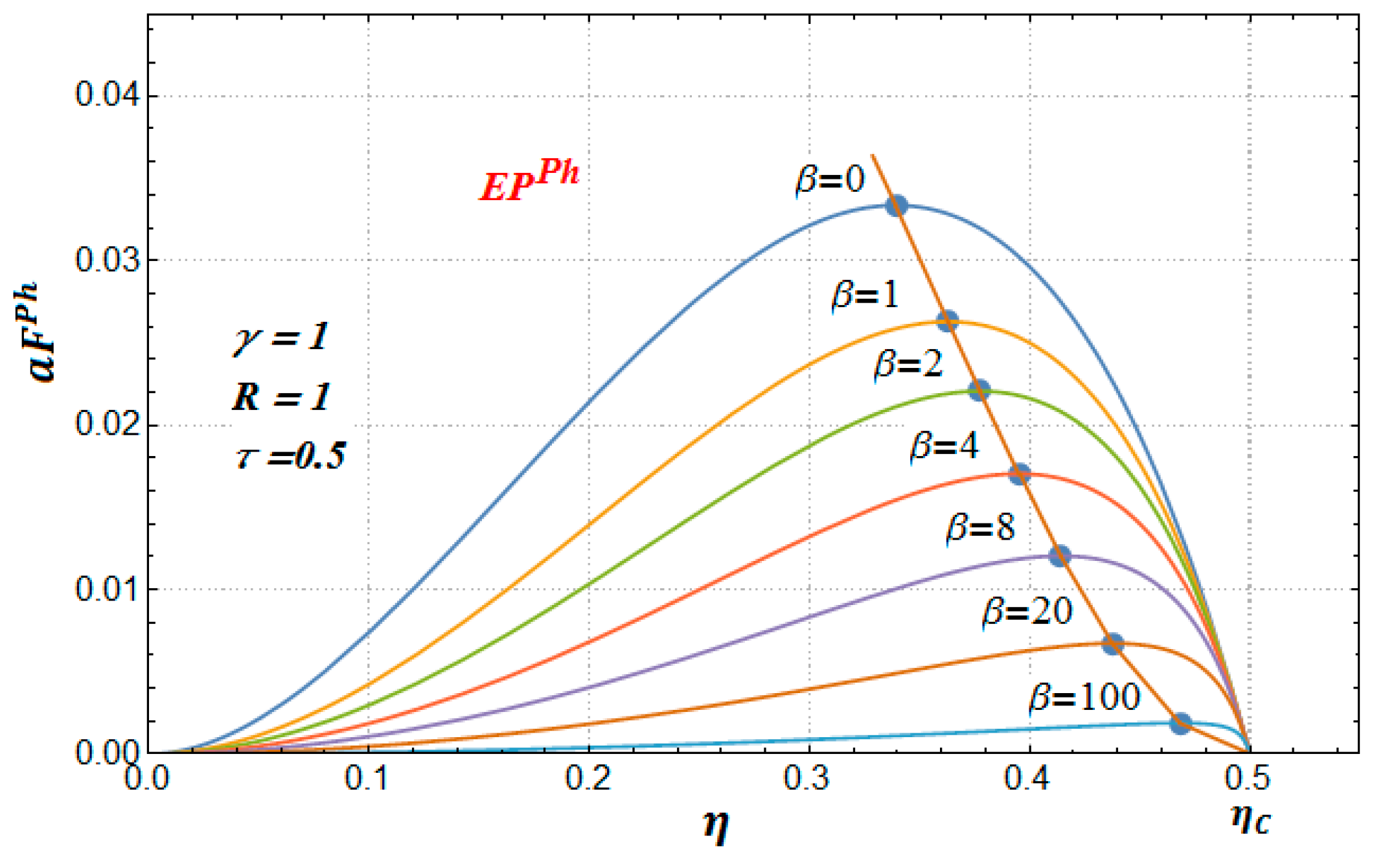
In Figure 4 and Figure 5, we show the behavior of $a{F}_{MP}^{SB-Ph}$, $a{F}_{EP}^{SB-Ph}$ and $a{F}_{ME}^{SB-Ph}$ for the case of a phenomenological ($Ph$) heat transfer law ($n=-1$ in Equations (18)–(20)) versus the internal efficiency for $R=1$, $\beta =0$ and $\tau =0.5$ (a similar behavior is found for the benefit functions for the case of the Stefan–Boltzmann law). 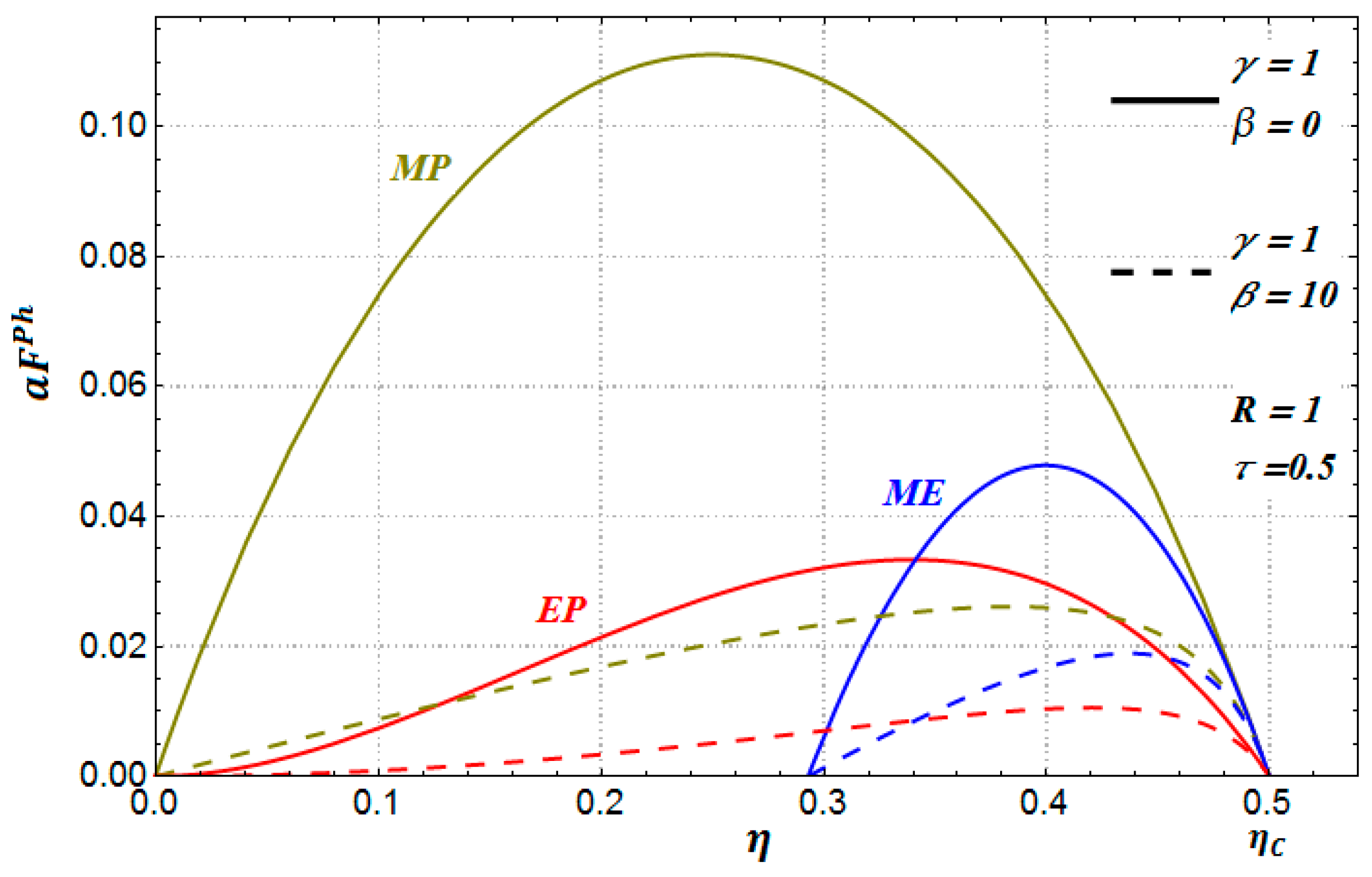We can see in Figure 5 and Figure 6 that these profit functions have a similar behavior to the Newton and the Dulong–Petit cases; that is, the benefits function also diminishes as the parameter $\gamma$ increases. In [11], it was shown that the maxima points of the MP profit function tend to the reversible limit (Carnot point) when the parameter $\beta$ tends to infinite. This same behavior occurs for the EP and ME profit functions. In Figure 6 we only show, as an example, the case of the EP profit function for several increasing values of the parameter $\beta$, and it is clear how the curve that contains the maxima points tend to the Carnot efficiency (${\eta }_C=0.5$, in this case).

In a similar way to the Newton and the Dulong–Petit cases, we can obtain the optimal efficiencies in terms of the parameter β (or $f$).

Analogously to Newton and Dulong–Petit laws, we can also obtain some analytical expressions for $\gamma =0$ for both Ph ($n=-1$) and SB radiation ($n=4$) laws. Therefore, under maximum power output, maximum efficient power and maximum ecological function conditions, we obtain, respectively,

$${\eta }_{MP}^{Ph}\left(\tau ,f,R\right)=\frac{R-\tau }{R(2-f)},$$

(21a)

$${\eta }_{EP}^{Ph}\left(\tau ,f,R\right)=\frac{\tau (f-3)}{R(f-1)-2\tau },$$

(21b)

$${\eta }_{ME}^{Ph}\left(\tau ,f,R\right)=\frac{R\left[(f-3)-(f-1)\tau \right]+2\tau }{2R(f-2)},$$

(21c)

and,

$${\eta }_{MP}^{S-B}\left(\tau ,f,R\right)=1-\frac{8(f-1)R\tau }{(4f-3)\tau +\sqrt{{(4f-3)}^2{\tau }^2+16R(1-f)\tau }},$$

(22a)

$${\eta }_{EP}^{S-B}\left(\tau ,f,R\right)=1-\frac{2(f-1)\tau -\sqrt{8(1-f)\tau R+(1-2f){\tau }^2}}{2R},$$

(22b)

$${\eta }_{ME}^{S-B}\left(\tau ,f,R\right)=1-\frac{(4f-3)\tau +\sqrt{{(4f-3)}^2{\tau }^2+8R(f-1)(1+\tau )\tau }}{2R}.$$

(22c)

Similarly as for the Newton heat transfer law, for a phenomenological heat transfer law when $f=0$ and $R=1$, from Equation (21a–c), we obtain the optimal efficiencies ${\eta }_{MP}=\left(1-\tau \right)/2$ previously reported by De Vos [24], ${\eta }_{EP}=\frac{3\tau }{1+2\tau }$ and ${\eta }_{ME}=3\left(1-\tau \right)/4$ (these last two expressions were previously published by Barranco-Jiménez [21]), for the Curzon-Ahlborn heat engine under maximum power output, maximum efficient power and maximum ecological function conditions, respectively.

3. Numerical Results: Environmental Impact

When we calculate the derivative of Equations (8)–(10), that is, ${\frac{d\left(a{F}_i\right)}{d\eta }|}_{{\eta }_i^{*}}$, for $i=MP,EP,ME$, we obtain equations of the form ${\frac{d\left(a{F}_i\right)}{d\eta }|}_{n_i}=H\left(\tau ,\beta ,\gamma ,R,{\eta }_i^{*}\right)$. Therefore, we have to solve numerically polynomial equations of the form,

$$H_i^{N-DP}=H_i^{N-DP}\left(\tau ,\beta ,\gamma ,R,{\eta }_i^{N-DP}\right)=0,$$

(23)

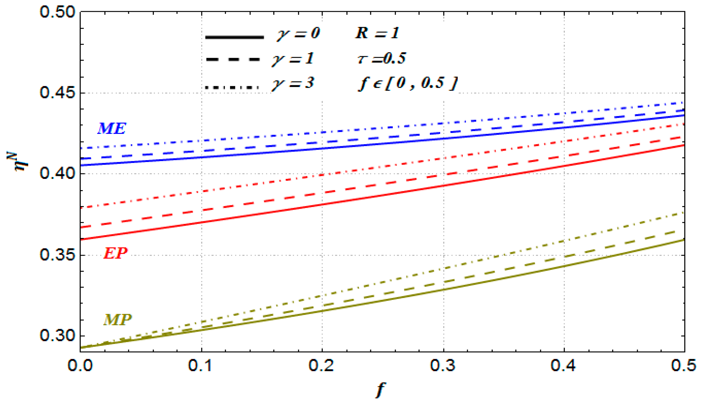
These previous expressions are not shown in explicit form because they are very large. Finally, using the expression for the fractional fuel cost $f$ [11,17] (see Equation (12)), we obtain the numerical optimal efficiencies in terms of the parameter $R$, the parameter $\tau$ and the economic parameters f and $\gamma$. In Figure 7, we show the optimal numerical efficiencies under maximum power, maximum efficient power and maximum ecological function conditions, respectively. In this Figure (see solid lines), we also show the optimal efficiencies given by Equations (13a), (14a) and (15a).

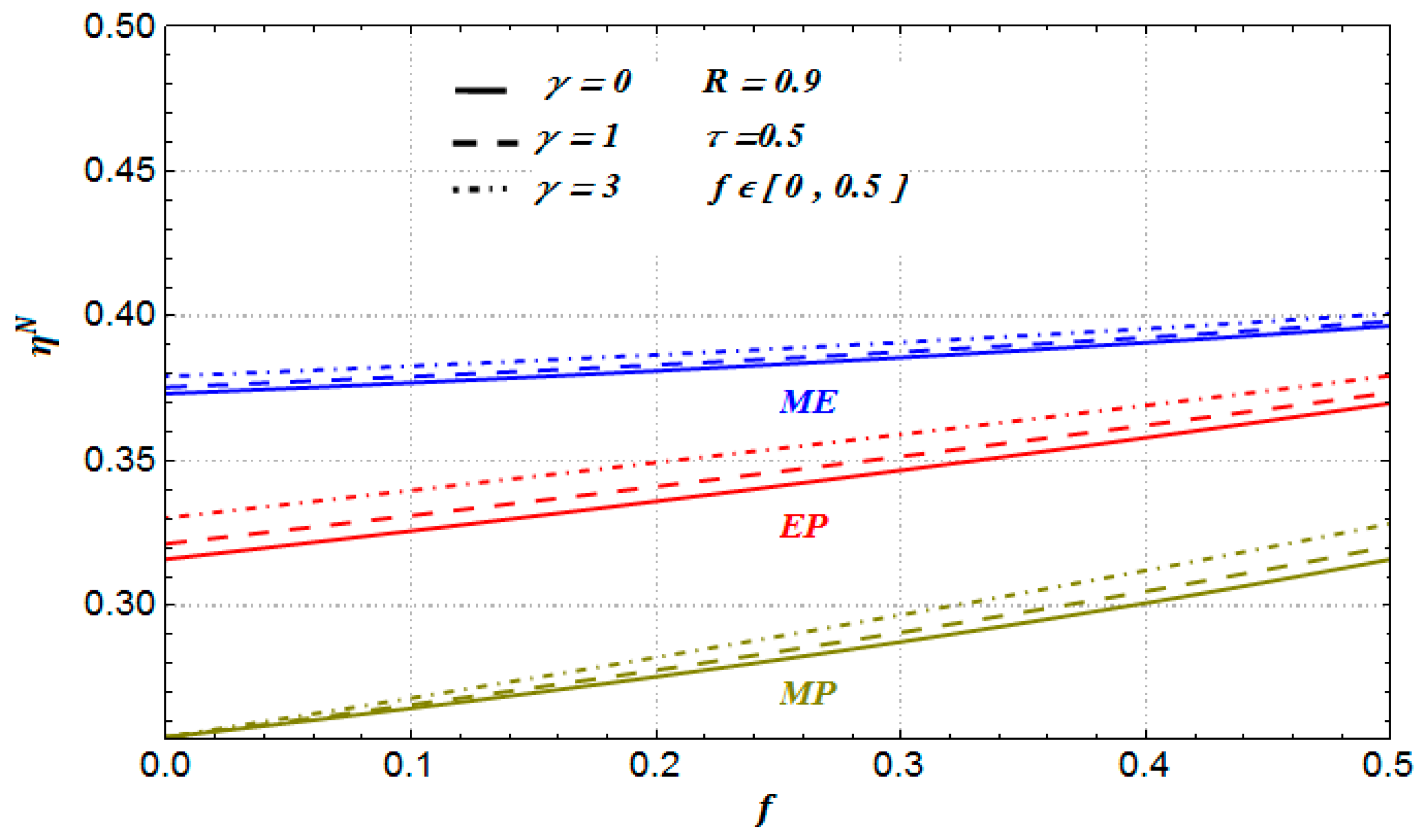
On the other hand, in Figure 8 we depict the corresponding optimal efficiencies against f for the Newtonian case, but with R = 0.9 < 1 (this case is a representative one of any nonendoreversible situation). As we can see in this case, the ${\eta }^N$ optimal values are all smaller than those corresponding to Figure 7. This behavior for R < 1 is present for any heat transfer law and any operating regime [21,40].

We can also see that the optimal efficiencies under the maximum ecological function regime (for all values of the parameters $R$, $\gamma$ and $f$ for the case of Newton heat transfer law, see Figure 7 and Figure 8) are greater than the optimal efficiencies under both maximum power output and maximum efficient power conditions, respectively. For the case of both phenomenological and Stefan–Boltzmann laws, the optimal efficiencies have a similar behavior with respect to the parameters $R$, $\gamma$ and $f$. Besides, all of these optimal efficiencies satisfy the following inequality:

$${\eta }_C>{\eta }_{ME}>{\eta }_{EP}>{\eta }_{MP}>{\eta }_{CA},$$

(24)

The previous inequality was recently obtained by Barranco-Jiménez et al. for the case of both endoreversible and nonendoreversible models of heat thermal engines [21,40]. In addition, we can see in Figure 2 and Figure 3 how the optimal efficiency under the maximum ecological function regime leads to a high reduction on the profits in comparison with those at maximum power output. However, this reduction is concomitant with a better efficiency for each value of the parameter $f$ (see Table 1 in [11] for fractional fuel costs for several kinds of fuels). This value of the efficiency provides a diminution of the energy rejected to the environment by the power plant. Therefore, the ecological criterion becomes an appropriate procedure for the search for insight into an engine’s performance for providing a less aggressive interaction with the environment. Therefore, we propose the following simplified analysis:

From the first law of thermodynamics we get,

$$Q_L=Q_H-W,$$

(25)

where $Q_L$ is the heat rejected to the environment by the power plant. For the cases of heat transfer of the Newton and Dulong–Petit types, when the power plant works under maximum power conditions by using Equations (3), (4) and (25), we get

$$Q_L\left({\eta }_{MP}^{*},\tau ,R\right)=g{T}_H^n\left(1-{\eta }_{MP}^n\right){\left(1-\frac{\tau }{R\left(1-{\eta }_{MP}^{*}\right)}\right)}^n.$$

(26)

In a similar way, the expressions when the power plant works under maximum ecological function and maximum efficient power conditions are, respectively,

$$Q_L\left({\eta }_{ME}^{*},\tau ,R\right)=g{T}_H^n\left(1-{\eta }_{ME}^n\right){\left(1-\frac{\tau }{R\left(1-{\eta }_{ME}^{*}\right)}\right)}^n,$$

(27)

$$Q_L\left({\eta }_{EP}^{*},\tau ,R\right)=g{T}_H^n\left(1-{\eta }_{EP}^n\right){\left(1-\frac{\tau }{R\left(1-{\eta }_{EP}^{*}\right)}\right)}^n.$$

(28)

The solutions of Equations (26)–(28) were obtained in a numerical manner similarly to the equations in Section 2. In our optimization, we consider different values for the maintenance of the power plant (parameter $\gamma$) and we can observe for each thermodynamic regime that while the $\gamma$ parameter increases, the heat rejected to the environment slightly diminishes, as it is shown in Figure 9.

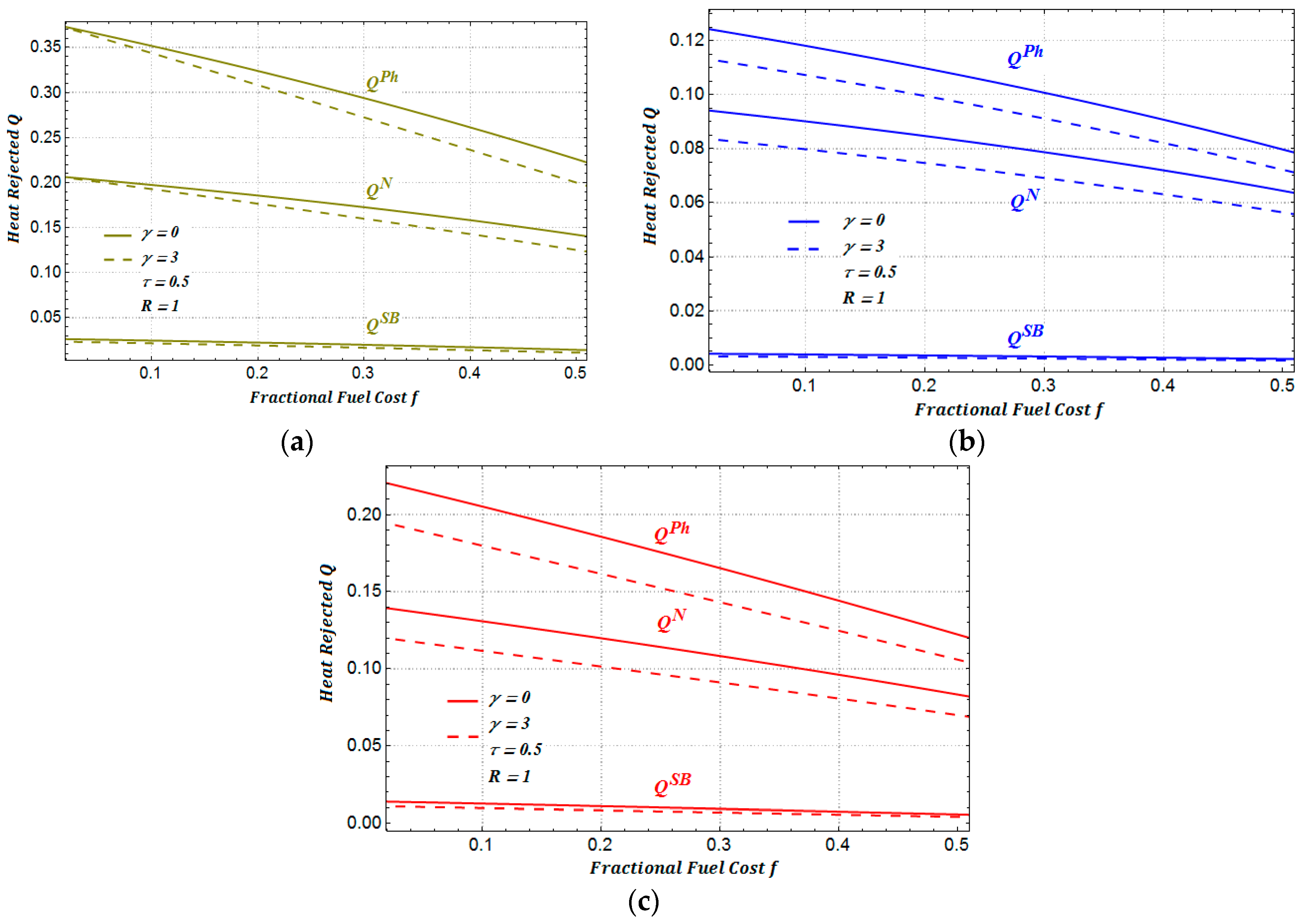
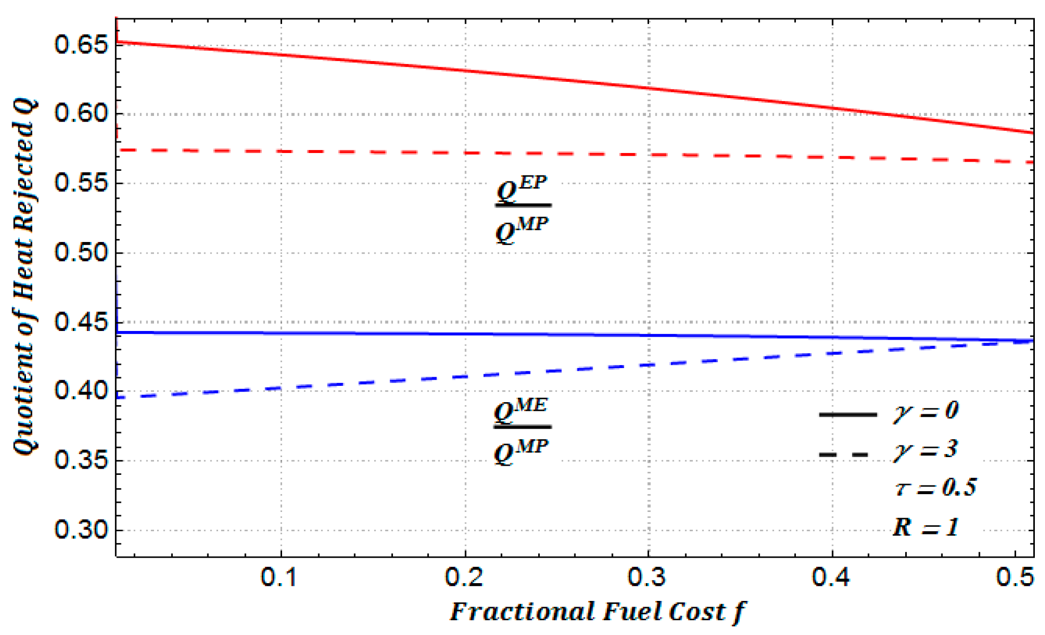
In Figure 9, we show the amount of heat rejected to the environment for each one of the three regimes of performance. As we can see, the heat rejected to the environment under the maximum ecological function presents a less aggressive impact to the environment in comparison with the other two regimes (see Figure 10a,b). We can also observe in Figure 10 that when the cost of the maintenance is taken into account, the rejected heat slightly diminishes in the three regimes of performance considered.

In Figure 11, we show the ratio between the amounts of heat rejected for a heat transfer law of the Dulong–Petit type.

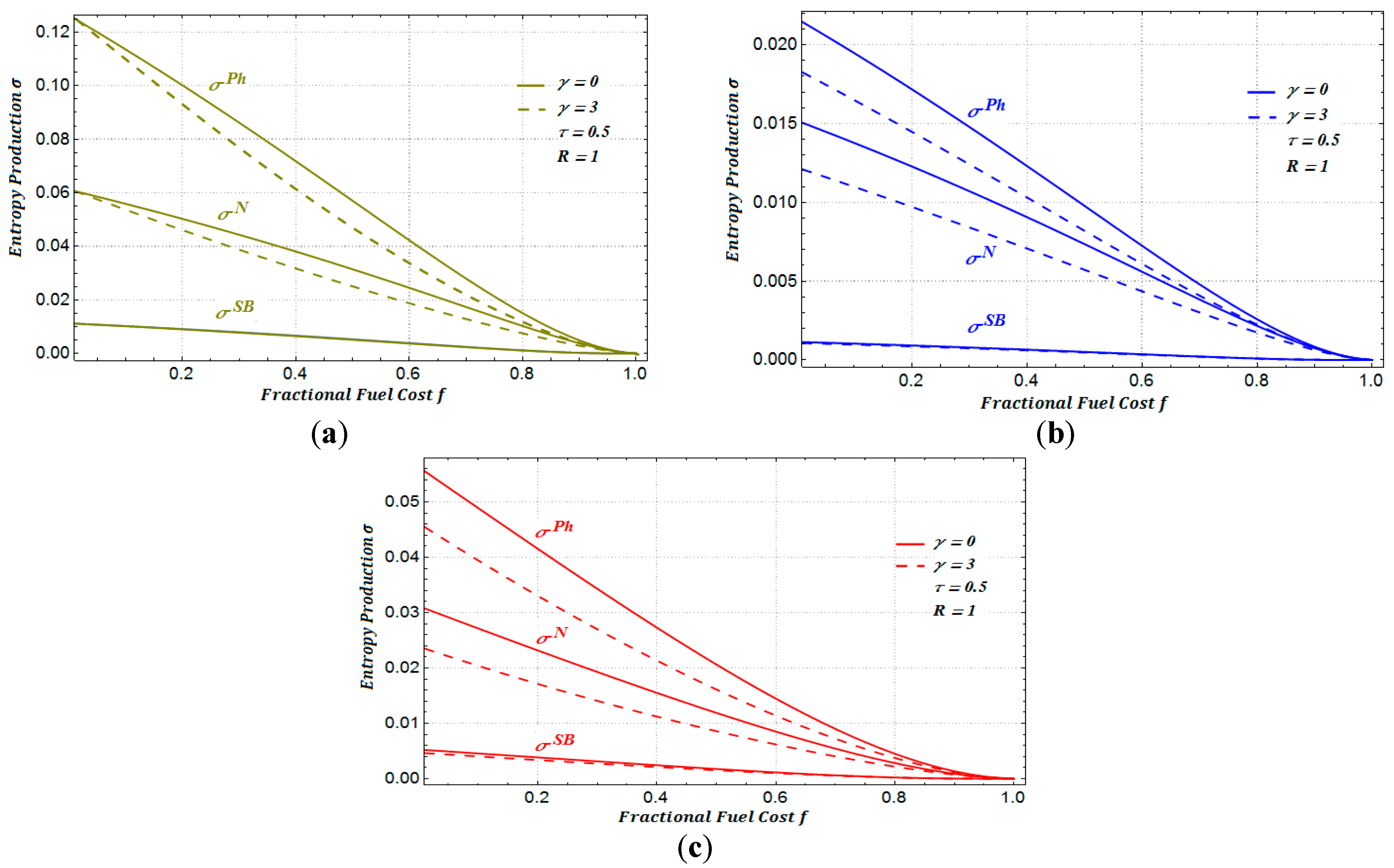
Furthermore, by applying the second law of thermodynamic (see Figure 1) we get,

$$\sigma =\frac{Q_H-W}{T_L}-\frac{Q_H}{T_H}.$$

(29)

Using Equations (1), (3) and (4) and after some algebraic manipulations, for the cases of heat transfer of the Newton and Dulong–Petit types, the entropy production under maximum power conditions can be calculated by the following expression:

$${\sigma }_{MP}\left({\eta }_{MP}^{*},\tau ,R\right)=\left(1-\tau -{\eta }_{MP}^{*}\right){\left(1-\frac{\tau }{R\left(1-{\eta }_{MP}^{*}\right)}\right)}^n.$$

(30)

Similarly to Equation (30), the expressions when the power plant works under maximum ecological function and maximum efficient power conditions are, respectively,

$${\sigma }_{ME}\left({\eta }_{ME}^{*},\tau ,R\right)=\left(1-\tau -{\eta }_{ME}^{*}\right){\left(1-\frac{\tau }{R\left(1-{\eta }_{ME}^{*}\right)}\right)}^n,$$

(31)

$${\sigma }_{EP}\left({\eta }_{EP}^{*},\tau ,R\right)=\left(1-\tau -{\eta }_{EP}^{*}\right){\left(1-\frac{\tau }{R\left(1-{\eta }_{EP}^{*}\right)}\right)}^n.$$

(32)

It is important to mention that all of the calculations were made in a numerical form. The behavior of the above equations can be observed in Figure 12. As can be seen in Figure 12b, the entropy production of the power plant when it is working under maximum ecological conditions is less than when it is working under maximum power conditions.

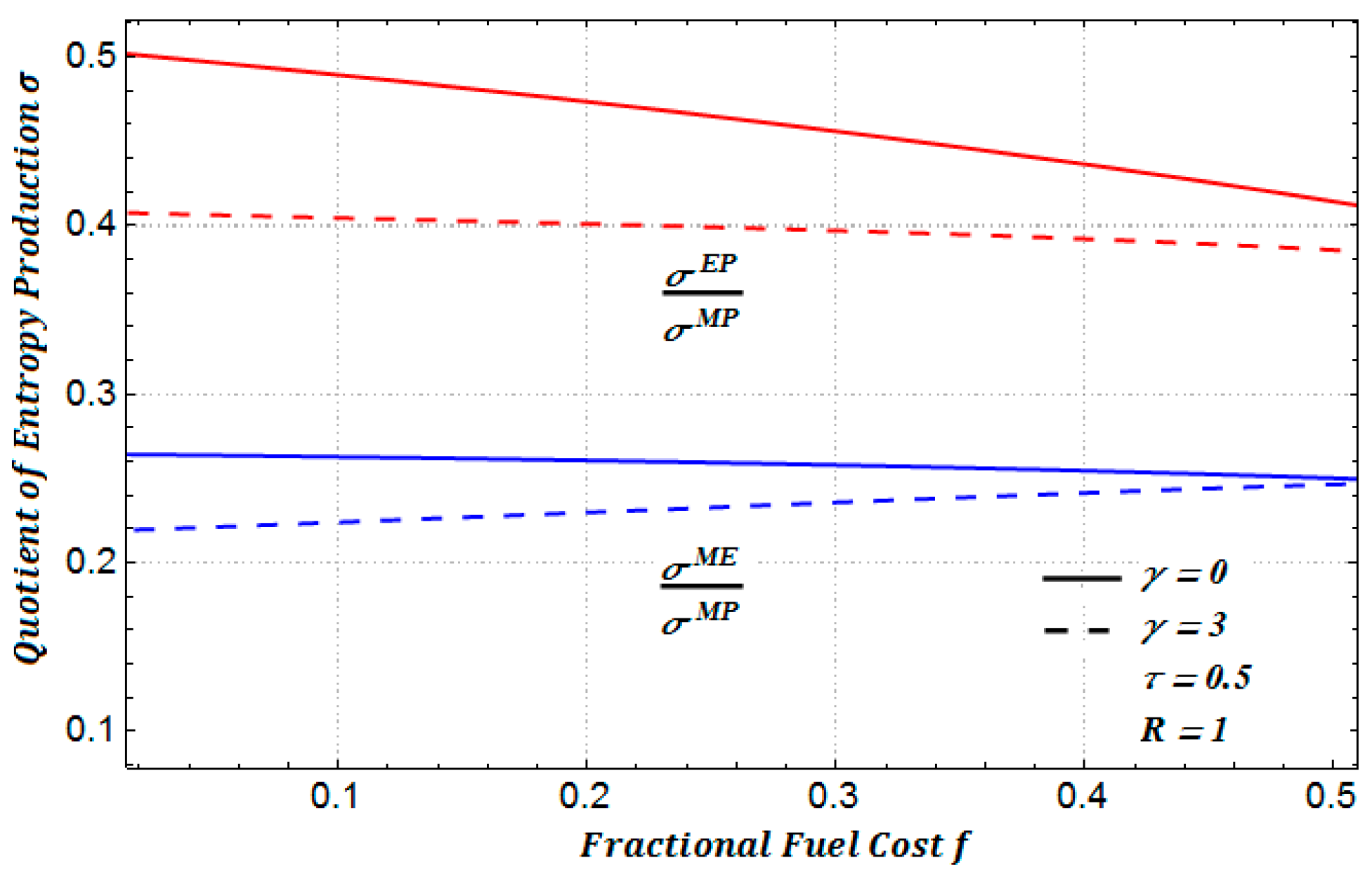
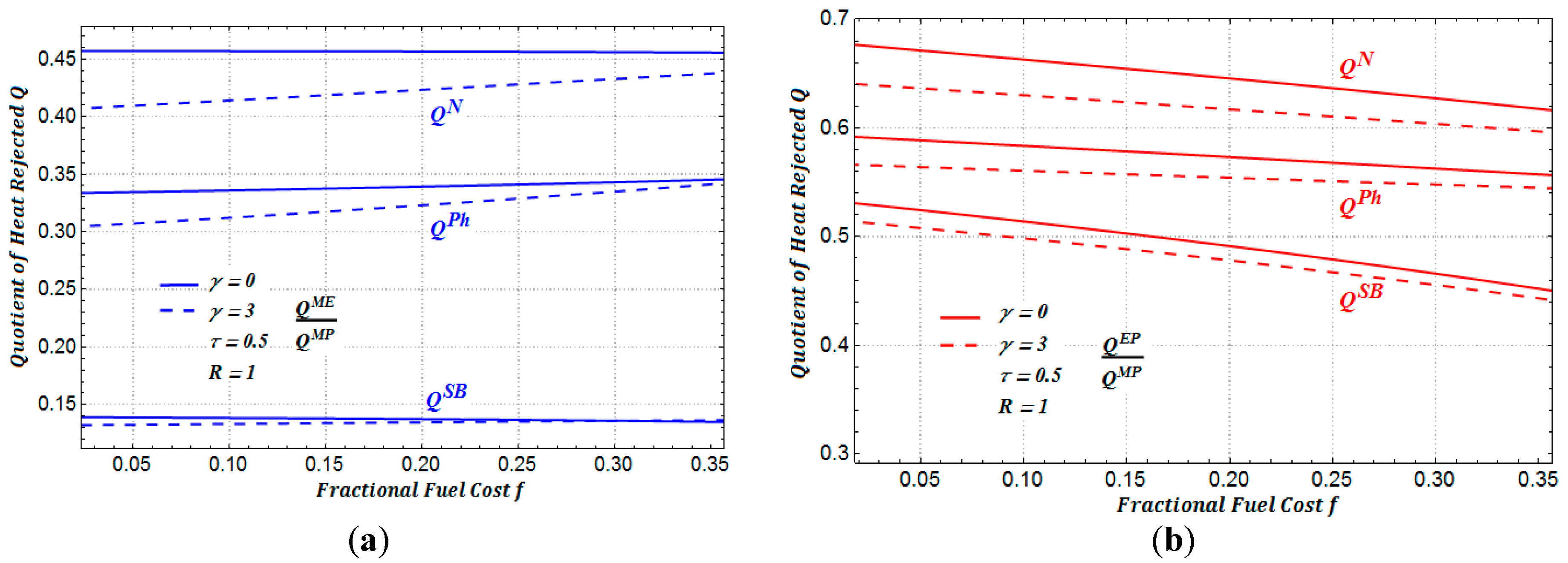
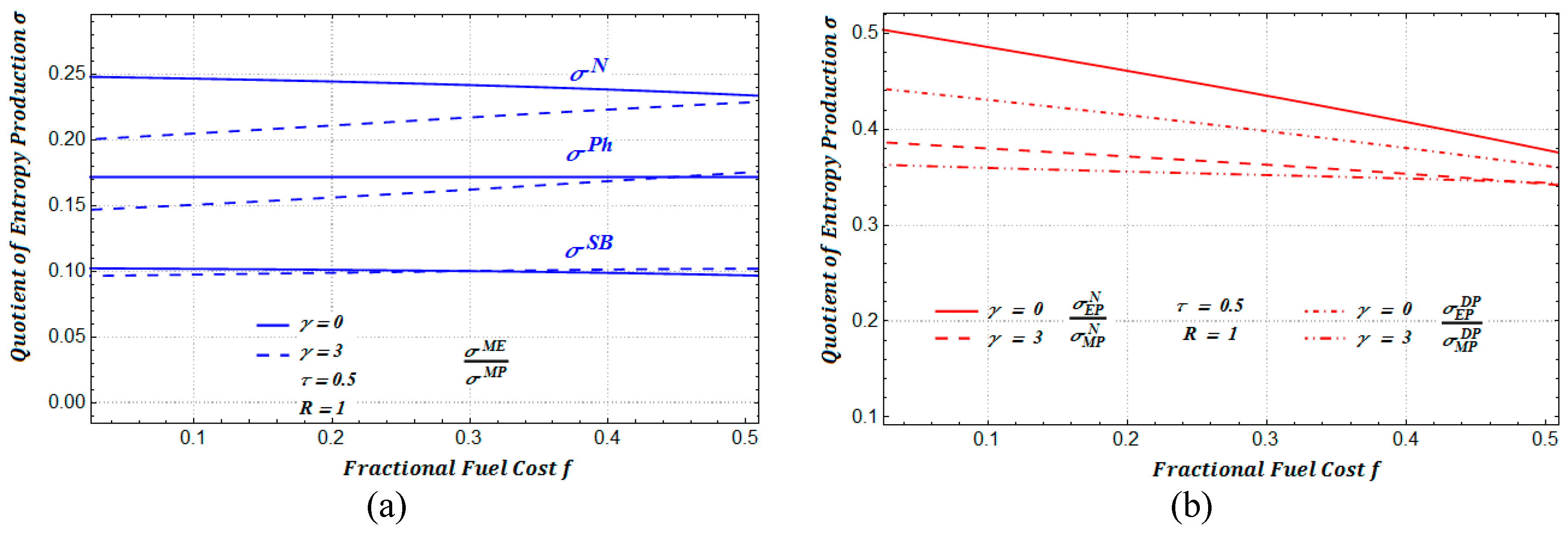
In Figure 13a, we show the ratio between the amounts of entropy production for two regimes: maximum ecological function and maximum power. In a similar manner, in Figure 13b, we show the ratio between the amounts of entropy production for maximum efficient power conditions and maximum power conditions. In addition, in Figure 14, we show the ratios of entropy production for a heat transfer of the Dulong–Petit type. In all of our numerical calculations we have attempted to use for the distinct involved parameters only typical values reported in the FTT literature.

4. Conclusions

In this work, we have made a thermoeconomic study of an irreversible simplified thermal power plant model (the so-called Novikov engine). This irreversible model modifies the results obtained by means of an endoreversible one due to the inclusion of the engine’s internal dissipation through the lumped parameter R (see Figure 7 and Figure 8). In our study, we use different heat transfer laws: the Newton’s law of cooling, the Stefan–Boltzmann radiation law, the Dulong–Petit’s law and another phenomenological heat transfer law. We also take into account a cost associated to the maintenance of the power plant which we assume as proportional to the power output of the plant. The inclusion of this new cost has a noticeable impact on the improvement of the optimal efficiencies of the plant model, nevertheless, the benefit functions diminish. This effect is only relevant when the plant model works under ME and EP regimes; however, when the plant model works at maximum power regime, the benefits diminish and the optimal efficiency practically does not change. We found that when the Novikov model maximizes the ecological function, it remarkably reduces the rejected heat to the environment in comparison to the rejected heat in the case of a power plant model working under the maximum power regime (see Figure 9, Figure 10 and Figure 11). In addition, we analyzed the effect of internal irreversibilities on the reduction of power output and on the total entropy production of the model. In summary, we have shown that the maximum ecological regime has more advantages in the way of thermoeconomic performance than the other mentioned operating regimes.