Optimization of Alpha-Beta Log-Det Divergences and their Application in the Spatial Filtering of Two Class Motor Imagery Movements

Abstract

The Alpha-Beta Log-Det divergences for positive definite matrices are flexible divergences that are parameterized by two real constants and are able to specialize several relevant classical cases like the squared Riemannian metric, the Steins loss, the S-divergence, etc. A novel classification criterion based on these divergences is optimized to address the problem of classification of the motor imagery movements. This research paper is divided into three main sections in order to address the above mentioned problem: (1) Firstly, it is proven that a suitable scaling of the class conditional covariance matrices can be used to link the Common Spatial Pattern (CSP) solution with a predefined number of spatial filters for each class and its representation as a divergence optimization problem by making their different filter selection policies compatible; (2) A closed form formula for the gradient of the Alpha-Beta Log-Det divergences is derived that allows to perform optimization as well as easily use it in many practical applications; (3) Finally, in similarity with the work of Samek et al. 2014, which proposed the robust spatial filtering of the motor imagery movements based on the beta-divergence, the optimization of the Alpha-Beta Log-Det divergences is applied to this problem. The resulting subspace algorithm provides a unified framework for testing the performance and robustness of the several divergences in different scenarios.

1. Introduction

Over the last few years, the use of specialized metrics and divergences measures in the successful design of dimensionality reduction techniques has been progressively acquiring much recognition [1,2,3,4,5]. There are numerous real scenarios and applications for which the parameters of interest belong to non-flat manifolds, and where the Euclidean geometry results are unsuitable to evaluate the similarities. Indeed, this is usual case in the comparison of probability density functions and also of their associated covariance matrices. The present contribution may be seen as a continuation of the work in [6], where we defined the Alpha-Beta Log-Det family of divergences between Symmetric and Positive Definite (SPD) matrices and studied its properties. The Alpha-Beta Log-Det family unifies under the same framework many existing Log-Det divergences and connects them smoothly, through intermediate versions, with the help of two real hyperparameters: α and β. In [7] a recent extension of the the Alpha-Beta Log-Determinant divergences was also proposed for the infinite-dimensional setting.

The evaluation of the Alpha-Beta Log-Det divergences depends on the generalized eigenvalues of the compared SPD matrices, and this makes its optimization non-trivial. In this paper, we motivate the use of these divergences with the illustrative application of dimensionality reduction in Brain-Computer Interface (BCI) and explain how to perform their optimization. The electroencephalogram (EEG) data has a typical high-dimensionality, a low signal to noise ratio and may have artifacts/outliers. The dimensionality reduction is then a necessary processing of the EEG signals for extracting those subspaces where the features have highest discriminative power.

Brain-Computer Interface has gained lots of interest in neuroscience and rehabilitation engineering. BCI [8,9] systems enable a person to operate external devices by using brain signals. The motor imagery (MI) based BCI systems are the most preferable BCI systems among others. It uses the brain signals of the MI movements as control commands for external devices without using the peripheral nervous system. During the imagination process, an alteration in the rhythmic activity of the brain can be observed in the mu and β rhythms at the corresponding area of the sensory-motor cortex. This phenomenon is known as event-related synchronization (ERS) or event-related desynchronization (ERD) [10]. The MI-based BCI systems use theses activities as control commands. Such a system can potentially serves as a communication aid for the people suffering from amyotrophic lateral sclerosis, multiple sclerosis and completely locked-in.

One of the most popular and efficient algorithms used for MI-based BCI applications is the common spatial pattern (CSP) algorithm [11]. It was first used to detect the abnormalities present in EEG signals [12] and later, was introduced in BCI applications [13]. The main objective of the CSP is to obtain the spatial filters by maximizing the variance of one class, at the same time minimizing that of the other class variance. It has been reported that this algorithm provides excellent classification accuracy for MI-based BCI systems. Besides, being the most popular method, its performance is easily affected by the presence of artifacts and nonstationarities. Since the computation of the spatial filters mainly depends on the covariance matrix, the presence of artifacts such as blinking of the eyes, eye movements and improper placement of the electrodes contribute to the poor computation of the covariance matrix which leads to the poor classification performance.

The main contributions of this work are the following:

• The existing link between the CSP method and the symmetric KL divergence (see [1]), is extended to the case of the minimax optimization of the AB log-det divergences. In absence of regularization, their solutions are shown to be equivalent whenever these methods apply the same divergence-based criterion for choosing the spatial filters. Although, in general, this is not the case when the CSP method adopts the popular practical criterion of a priori fixing the number of spatial filters for each class, we show that the equivalence with the solution of the optimization of AB log-det divergences can be still preserved if a suitable scaling factor κ is used in one of the arguments of the divergence.
• The details on how to perform the optimization of the AB log-det divergence are presented. The explicit expression of the gradient of this divergence with respect to the spatial filters is obtained. Expression which generalizes and extends the gradient of several more established well-known divergences, for instance, the gradient of the Alpha–Gamma divergence and the gradient of the Kullback–Leibler divergence between SPD matrices.
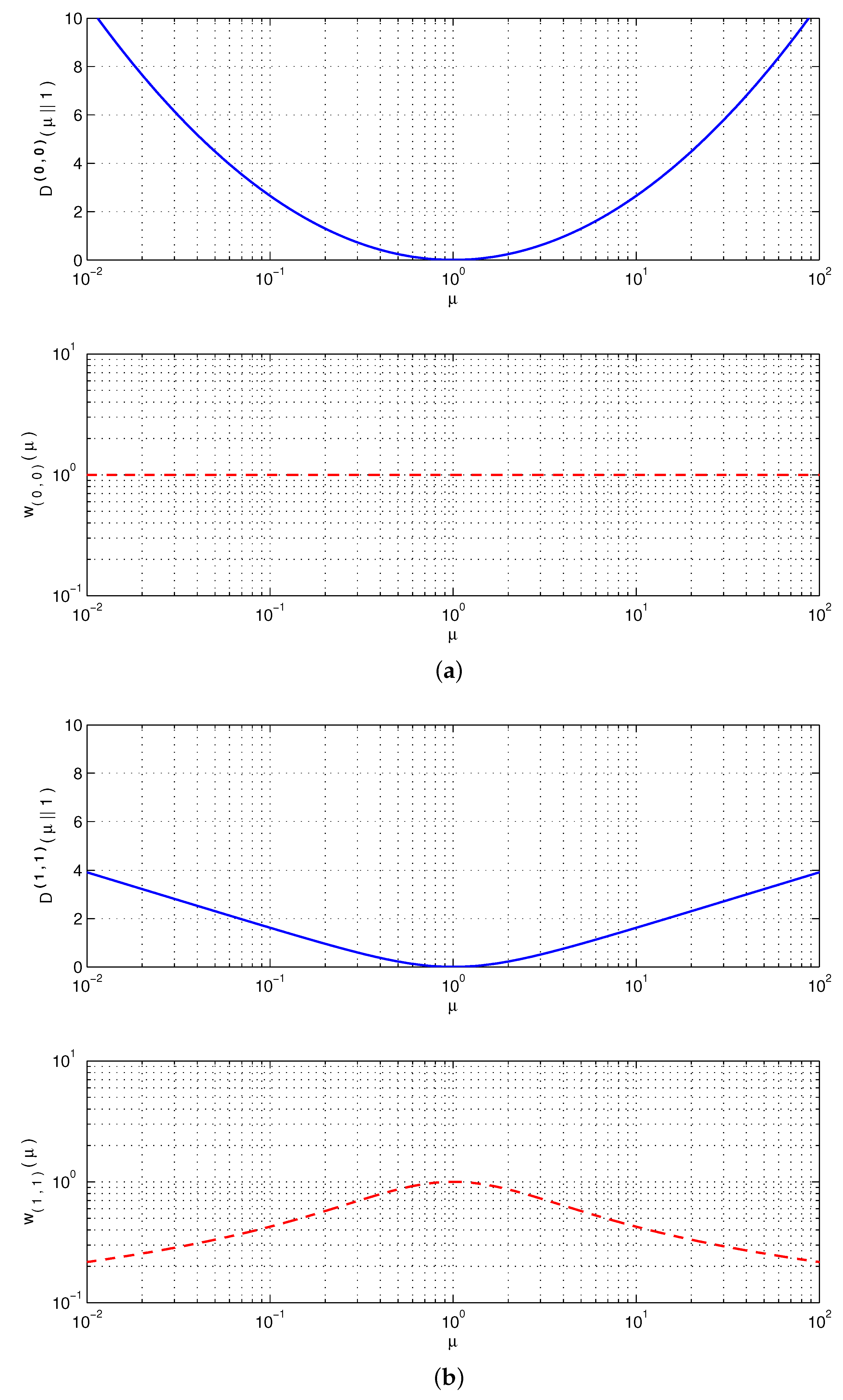
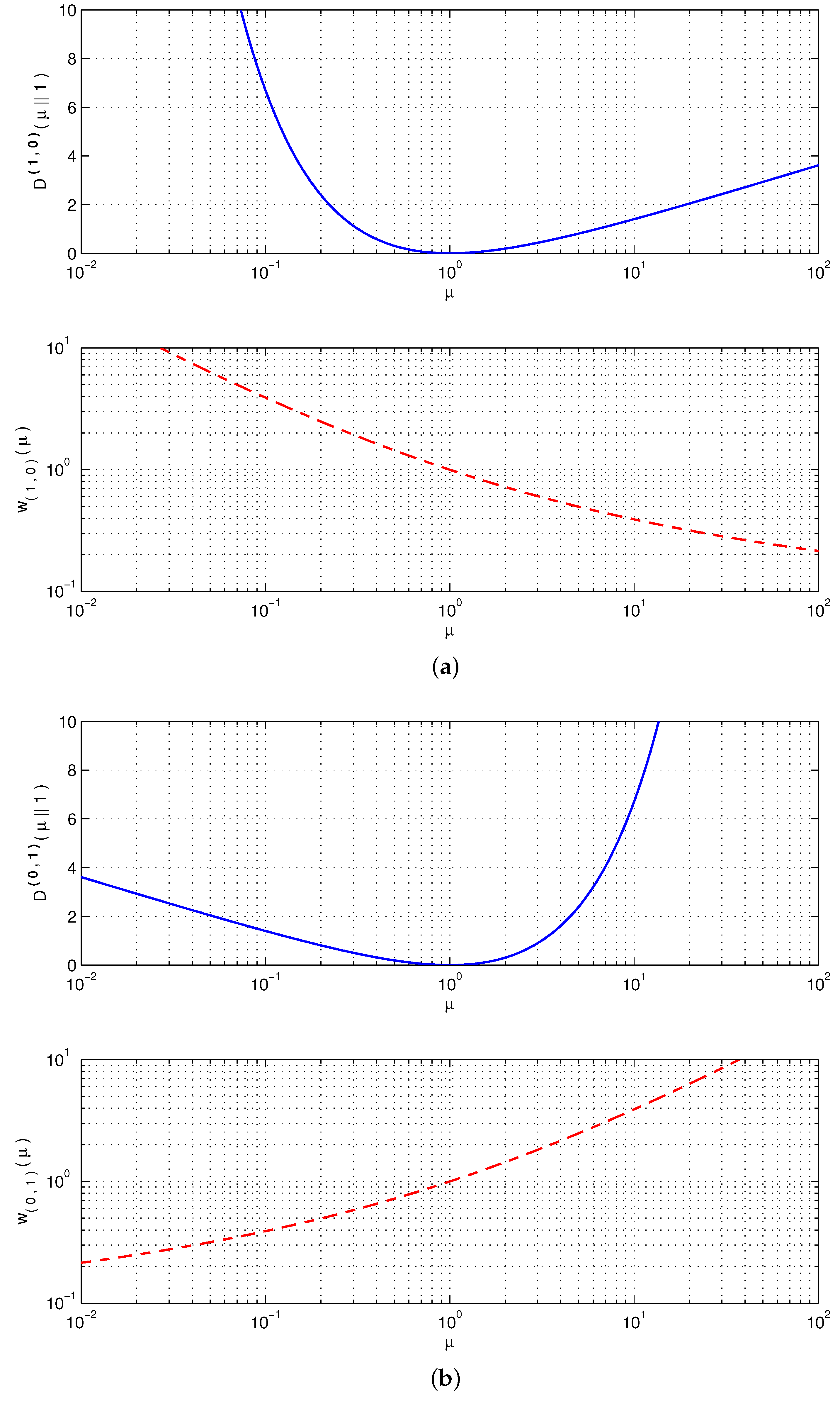
• The robustness property of the AB log-det divergence with respect to outliers has been analyzed. The study reveals that the hyperparameters of the divergence can be chosen to underweight or overweight, at convenience, the influence of the larger and smaller generalized eigenvalues in the estimating equations.
• Motivated by the success of criteria based on the Beta divergence [1] in the robust spatial filtering of the motor imagery movements, in this work, we consider the use of a criterion based on AB log-det divergences for the same purpose. A subspace optimization algorithm based on regularized AB log-det divergences is proposed for obtaining the relevant subset of spatial filters. Some exemplary simulations illustrate its robustness over synthetic and real datasets.

This article is organized as follows: Section 2 presents the fundamental model of the observations and paper notation. Section 3 reviews the CSP algorithm while Section 4 discusses CSP via the divergence optimization. In Section 5, we present the family of AB log-det divergences and provide a new upper-bounds and conditions for the equivalence between this divergence optimization and the robust CSP solution. Section 6 explains how to obtain closed-form formulas for computing the gradient of the AB log-det divergence, which is useful for its optimization. The analysis of the robustness of the divergence in terms of its hyperparameters is the objective of Section 7. Section 8 briefly reviews several related techniques, while Section 9 presents the regularized version of the criterion based on AB log-det divergences, as well as, the subspace algorithm that optimizes it. Section 10 presents the experimental datasets, the steps involved in the preprocessing, feature extraction and classification. The results of the simulations are presented and discussed in Section 11. Finally, the paper summarizes main results in Section 12.

2. Notation and Model of the Measurements

Throughout this paper, the following notations are adopted. Vectors are typically denoted by bold letters, the capital bold letters are reserved for the matrices, while the random variables appear in italic capital letters. The operators $\lfloor ·\rfloor$ and $\lceil ·\rceil$ round the value of their argument to the nearest lower and higher integers respectively. All the covariance matrices, which are denoted by $Cov(·)$, are assumed to be positive definite and hence invertible.

Let us now describe the statistical model of the observations. As usual, the raw EEG observations are initially preprocessed by a bandpass filter that retains the activity in the bands of the mu and β rhythms and are later normalized for each trial so as to keep their total spatial power constant. One can define a statistical model of these “normalized” observations as $\mathit{x}(t)={[x_1(t),\dots ,x_n(t)]}^T$ conditioned on the true imagery movement, which here will be represented by a member of the class $c\in \{c_1,c_2\}$. In general, the EEG observations are noisy and high-dimensional, while the number of recorded trials is quite limited. Therefore, the learning of the discriminative features is quite sensitive to overfitting, a situation that would severely degrade the prediction accuracy over test samples. In this case, it is worth sacrificing the bias by choosing a simpler (less complex) model in which parameters can be estimated with a smaller variance. For this reason, we adopt usual convention [14] of considering the observations from each class as drawn from the independent and identically distributed (i.i.d.) Gaussian random vectors as represented as $\mathit{X}|c$ of zero mean and with covariance matrix as $Cov(\mathit{X}|c)$, which in turn is set equal to the sample covariance matrix of the class, i.e.,

$$\begin{array}{c}\hfill Cov(\mathit{X}|c)=Cov(\mathit{x}|c)\mathrm{for}c\in \{c_1,c_2\}.\end{array}$$

(1)

The observations are then modeled by the mixture distribution

$$\begin{array}{ccc}\hfill p(\mathit{x})& =& p(c_1)p(\mathit{x}|c_1)+p(c_2)p(\mathit{x}|c_2),\hfill \end{array}$$

(2)

where $p(c)$ refers to the sample probabilities of each class in the training data. When $\overline{\mathit{x}}$ denotes the sample mean of the observations, their sample covariance matrix is obtained by

$$\begin{array}{}(3)& \hfill Cov(\mathit{x})& =& \frac{1}{T}{\displaystyle \sum _{t=1}^T}\left(\mathit{x}(t)-\overline{\mathit{x}}\right){\left(\mathit{x}(t)-\overline{\mathit{x}}\right)}^T\hfill (4)& & =& p(c_1)Cov(\mathit{x}|c_1)+p(c_2)Cov(\mathit{x}|c_2).\hfill \end{array}$$

and its eigenvalue decomposition is

$$\begin{array}{ccc}\hfill Cov(\mathit{x})& =& {\mathbf{U}}_1\mathbf{\Delta }{\mathbf{U}}_1^T\hfill \end{array}$$

(5)

where Δ and ${\mathbf{U}}_1$, respectively denote the matrix of eigenvalues and eigenvectors of $Cov(\mathit{x})$.

We define ${\mathit{w}}_i={[w_{1i},w_{2i},.....,w_{pi}]}^T$ as the vector with the coefficients of the i-th-esime spatial filter for $i=1,\dots ,p$. The collection of p spatial filters forms the overall filter matrix $\mathbf{W}=[{\mathit{w}}_1,{\mathit{w}}_2.....{\mathit{w}}_p]$, which is used to reduce the dimensionality of the observations by projecting them onto the p-dimensional subspace spanned by the filter outputs

$$\begin{array}{c}\hfill \mathit{y}={\mathbf{W}}^T\mathit{x}\in {\mathbb{R}}^p,\end{array}$$

(6)

where $p\ll n$. The model for the estimated conditional distribution $p(\mathit{y}|c)$ is a multidimensional Gaussian of zero mean and covariance matrix $Cov(\mathit{Y}|c)={\mathbf{W}}^{T}Cov(\mathit{x}|c)\mathbf{W}$, i.e., for each class

$$\begin{array}{c}\hfill \mathit{Y}|c\sim \mathcal{N}(\mathbf{0},{\mathbf{W}}^{T}Cov(\mathit{x}|c)\mathbf{W}).\end{array}$$

(7)

3. The Common Spatial Patterns Algorithm

The development of the CSP algorithm as a technique for feature selection in classification problems can be traced back to the work of [11], while later, [12,13] considered its practical application for the study of EEG signals. This technique exploits the event-related desynchronization during the limbs movement imagination process that alters the rhythmic activity in a class dependent area of the motor cortex. The objective of the algorithm is to obtain a set of most discriminative spatial filters, i.e., those that hierarchically maximize the output activity of one class, while at the same time; they minimize the activity of the other class. Since only the direction of the spatial filters (i.e., not the scale) are of interest, the technique starts with a linear transformation $\mathit{y}={\mathbf{W}}^T\mathit{x}$ that whitens the sample covariance of the outputs

$$\begin{array}{}(8)& \hfill Cov(\mathit{y})& =& p(c_1)Cov(\mathit{y}|c_1)+p(c_2)Cov(\mathit{y}|c_2)\hfill (9)& & =& {\mathbf{W}}^{T}Cov(\mathit{x})\mathbf{W}\hfill (10)& & =& {\mathbf{I}}_p.\hfill \end{array}$$

With the help of the eigenvalue decomposition of $Cov(\mathit{x})$, the general expression of the spatial filter matrix that preserves the whitening constraint can be found as

$$\begin{array}{c}\hfill {\mathbf{W}}^T={\mathbf{\Omega }}^T{\mathbf{\Delta }}^{-\frac{1}{2}}{\mathbf{U}}_1^T.\end{array}$$

(11)

Note that $\mathbf{W}\in {\mathbb{R}}^{n\times p}$ is specified up to the ambiguity in the choice of the semi-orthogonal matrix $\mathbf{\Omega }\in {\mathbb{R}}^{n\times p}$ (i.e., ${\mathbf{\Omega }}^T\mathbf{\Omega }={\mathbf{I}}_p$) which parameterizes the relevant degrees of freedom for finding the most discriminative directions. Then, the objective of the CSP criterion [11] is implemented by first choosing one part of the spatial filters from the constrained maximization of the conditional covariances of the outputs of the first class

$$\begin{array}{ccc}\hfill {\mathit{w}}_i& =& arg\underset{\mathit{w}}{max}{\mathit{w}}^{T}Cov(\mathit{x}|c_1)\mathit{w}i=1,\dots ,k,\hfill \end{array}$$

(12)

and later choosing the other part of the filters to hierarchically maximize the conditional covariances of the outputs of the second class

$$\begin{array}{ccc}\hfill {\mathit{w}}_i& =& arg\underset{\mathit{w}}{max}{\mathit{w}}^{T}Cov(\mathit{x}|c_2)\mathit{w}i=k+1,\dots ,p,\hfill \end{array}$$

(13)

where, in both cases, the maximization with respect to the spatial filters takes place under the whitening or ($Cov(\mathit{x})$-orthonormality) constraints

$$\begin{array}{c}\hfill {\mathit{w}}_i^{T}Cov(\mathit{x}){\mathit{w}}_j={\delta }_{ij}\forall j\le i.\end{array}$$

(14)

The number of spatial filters k that hierarchically maximize (12) can be determined by a chosen filter selection policy. For simplicity, in most cases it is usually set k close to $\frac{p}{2}$ with the aim to balance the number of spatial filters devoted to each of the classes.

The maximization in (12) can be alternatively posed as the constrained optimization of the quotient

$$\begin{array}{ccc}\hfill {\mathit{w}}_i& =& arg\underset{\mathit{w}}{max}\frac{{\mathit{w}}^{T}Cov(\mathit{x}|c)\mathit{w}}{{\mathit{w}}^{T}Cov(\mathit{x})\mathit{w}}\mathrm{subject}\mathrm{to}{\mathit{w}}^{T}Cov(\mathit{x})\mathit{w}={\delta }_{ij}\forall j\le i\hfill \end{array}$$

(15)

which, in terms of the transformed and normalized spatial vectors

$$\begin{array}{c}\hfill {\mathit{r}}_i=\frac{{(Cov(\mathit{x}))}^{\frac{1}{2}}{\mathit{w}}_i}{{\parallel {(Cov(\mathit{x}))}^{\frac{1}{2}}{\mathit{w}}_i\parallel }_2},\end{array}$$

(16)

is rewritten as a quadratic optimization under orthogonality constraints

$$\begin{array}{c}\hfill {\mathit{w}}_i={(Cov(\mathit{x}))}^{-\frac{1}{2}}\times arg\underset{\mathit{r}}{max}\left\{{\mathit{r}}^T{(Cov(\mathit{x}))}^{-\frac{1}{2}}Cov(\mathit{x}|c){(Cov(\mathit{x}))}^{-\frac{1}{2}}\mathit{r}\right\}\mathrm{s}.\mathrm{t}.{\mathit{r}}^T{\mathit{r}}_j={\delta }_{ij}\forall j\le i\end{array}$$

(17)

At this point, the straightforward application of the Courant–Fisher–Weyl minimax principle ([15], p. 58) yields the variational description of the desired spatial filters as the minimax solution of the Rayleigh quotients for each class

$$\begin{array}{}(18)& \hfill {\mathit{w}}_i& =& {(Cov(\mathit{x}))}^{-\frac{1}{2}}\times arg\underset{dim\{\mathcal{R}\}=n-i+1}{min}\underset{\stackrel{\mathit{r}\in \mathcal{R}}{\parallel \mathit{r}\parallel =1}}{max}\left\{{\mathit{r}}^T{(Cov(\mathit{x}))}^{-\frac{1}{2}}Cov(\mathit{x}|c){(Cov(\mathit{x}))}^{-\frac{1}{2}}\mathit{r}\right\}\hfill (19)& & =& arg\underset{dim\{\mathcal{W}\}=n-i+1}{min}\underset{\mathit{w}\in \mathcal{W}}{max}\frac{{\mathit{w}}^{T}Cov(\mathit{x}|c)\mathit{w}}{{\mathit{w}}^{T}Cov(\mathit{x})\mathit{w}}\hfill (20)& & =& arg\underset{dim\{\mathcal{W}\}=n-i+1}{min}\underset{\mathit{w}\in \mathcal{W}}{max}\frac{Cov(y_i|c)}{Cov(y_i)}.\hfill \end{array}$$

By the same principle, the generalized eigenvectors ${\mathit{v}}_i^{(c)}$ of the matrix pencil ($p(c)$$Cov(\mathit{y}|c)$, $Cov(\mathit{y})$), are the minimax solutions of the Rayleigh quotient, while the values that takes the criterion at these solutions are the generalized eigenvalues

$$\begin{array}{c}\hfill {\lambda }_i^{(c)}=p(c)\frac{{\mathit{v}}_i^{(c)T}Cov(\mathit{x}|c){\mathit{v}}_i^{(c)}}{{\mathit{v}}_i^{(c)T}Cov(\mathit{x}){\mathit{v}}_i^{(c)}}=p(c)\underset{dim\{\mathcal{W}\}=i}{min}\underset{\mathit{w}\in \mathcal{W}}{max}\frac{{\mathit{w}}^{T}Cov(\mathit{x}|c)\mathit{w}}{{\mathit{w}}^{T}Cov(\mathit{x})\mathit{w}},\end{array}$$

(21)

which are sorted according to the descent in their magnitude, ${\lambda }_1^{(c)}\ge {\lambda }_2^{(c)}\ge \dots \ge {\lambda }_n^{(c)}$.

The generalized eigenvectors of the two quotients (one for each class) coincide, except for their ordering which are reversed [11], i.e., ${\mathit{v}}_i^{(c_1)}={\mathit{v}}_{n-i+1}^{(c_2)}$, while the weighted sum of generalized eigenvalues is bounded by

$$\begin{array}{c}\hfill {\lambda }_i^{(c_1)}+{\lambda }_{n-i+1}^{(c_2)}=\frac{{\mathit{v}}_i^{(c_1)T}\left(p(c_1)Cov(\mathit{x}|c_1)+p(c_2)Cov(\mathit{x}|c_2)\right){\mathit{v}}_i^{(c_1)}}{{\mathit{v}}_i^{(c_1)T}Cov(\mathit{x}){\mathit{v}}_i^{(c_1)}}=1.\end{array}$$

(22)

Therefore, a direction of maximum variance for one class will simultaneously minimize the variance of the other class, and vice versa. Hence, the standard CSP solution is obtained when the spatial filters match with the principal and minor eigenvectors of the generalized eigendecomposition problem [11,12,13]

$$Cov(\mathit{x}|c_1){\mathit{v}}_i^{(c_1)}={\lambda }_i^{(c_1)}Cov(\mathit{x}){\mathit{v}}_i^{(c_1)}i=1,\dots ,n.$$

(23)

After sorting the eigenvalues according to its magnitude, CSP explicitly selects k spatial filters ${\mathit{v}}_i^{(c_1)}$ from the principal eigenvectors and $p-k$ spatial filters from the minor eigenvectors, to form the spatial filter matrix

$$\begin{array}{}(24)& \hfill {\mathbf{W}}_{CSP}& \equiv & [{\mathit{w}}_1,{\mathit{w}}_2.....{\mathit{w}}_p]\hfill (25)& & =& [{\mathit{v}}_1^{(c_1)},\dots ,{\mathit{v}}_k^{(c_1)},{\mathit{v}}_{n-(p-k)+1}^{(c_1)},\dots ,{\mathit{v}}_n^{(c_1)}].\hfill \end{array}$$

4. The Divergence Optimization Interpretation of CSP

Under the appropriate selection policy for the number of spatial filters for each class, the solution obtained by the CSP algorithm admits an interpretation in terms of the optimization divergence measures (here denoted by $Div(·\parallel ·)$) between the Gaussian pdfs outputs for each class

$$\begin{array}{ccc}\hfill {\mathit{w}}_i& =& arg\underset{dim\{\mathcal{W}\}=n-i+1}{min}\underset{\mathit{w}\in \mathcal{W}}{max}Div(p(y_i|c_1)\parallel p(y_i|c_2)),\hfill \end{array}$$

(26)

except for a probable permutation in the ordering of some of the spatial filters.

The problem can be formulated using the following optimization problem

$$\begin{array}{ccc}\hfill {\mathit{w}}_i& =& arg\underset{dim\{\mathcal{W}\}=n-i+1}{min}\underset{\mathit{w}\in \mathcal{W}}{max}D(Cov(y_i|c_1)\parallel Cov(y_i|c_2))\hfill \end{array}$$

(27)

where $D(·\parallel ·)$ refers to a divergence between the covariances of the conditional densities of the outputs. As a consequence of the assumption of zero mean Gaussian densities, the covariances are the only necessary statistics that summarize all the relevant information of the conditional data.

In particular, the solution of the CSP algorithm was linked in [1,11,16,17] with the optimization of the symmetric Kullback–Leibler divergence (sKL)

$$\begin{array}{}(28)& \hfill Di{v}_{{}_{sKL}}(p(y_i|c_1)\parallel p(y_i|c_2))& =& \int p(y_i|c_1)log\frac{p(y_i|c_1)}{p(y_i|c_2)}d{y}_i+\int p(y_i|c_2)log\frac{p(y_i|c_2)}{p(y_i|c_1)}d{y}_i,\hfill (29)& & =& \int (p(y_i|c_1)-p(y_i|c_2))log\frac{p(y_i|c_1)}{p(y_i|c_2)}d{y}_i.\hfill \end{array}$$

This divergence measures can be simplified to the symmetric Kullback–Leibler (sKL) divergence between the class conditional covariances

$$\begin{array}{}(30)& \hfill Di{v}_{{}_{sKL}}(p(y_i|c_1)\parallel p(y_i|c_2))& =& \frac{1}{2}\frac{Cov(y_i|c_1)}{Cov(y_i|c_2)}+\frac{1}{2}\frac{Cov(y_i|c_2)}{Cov(y_i|c_1)}-1\hfill (31)& & \equiv & D_{{}_{sKL}}(Cov(y_i|c_1)\parallel Cov(y_i|c_2)).\hfill \end{array}$$

In this paper, we propose an extension of the existing KL to the criterion of the Alpha-Beta log-det divergence (AB log-det) between the class-conditional covariances defined as [6]

$$\begin{array}{ccc}\hfill D_{AB}^{(\alpha ,\beta )}(Cov(y_i|c_1)\parallel Cov(y_i|c_2))& =& \frac{1}{\alpha \beta }log{\left|\frac{\alpha {\left(\frac{Cov(y_i|c_1)}{Cov(y_i|c_2)}\right)}^{\beta }+\beta {\left(\frac{Cov(y_i|c_2)}{Cov(y_i|c_1)}\right)}^{\alpha }}{\alpha +\beta }\right|}_{+}\hfill \\ \hfill \\ & & \mathrm{for}\alpha \ne 0,\beta \ne 0,\alpha +\beta \ne 0,\hfill \end{array}$$

(32)

where

$$\begin{array}{c}\hfill {|x|}_{+}=\left\{\begin{array}{cc}x\hfill & x\ge 0,\hfill \\ 0,\hfill & x<0,\hfill \end{array}\right.\end{array}$$

(33)

denotes the non-negative truncation operator. When the arguments covariances are scalars and $\alpha ,\beta >0$, the AB log-det divergence can also be rewritten as the logarithmic ratio between the weigthed arithmetic mean of the scaled covariances ($Co{v}^{\alpha +\beta }(y_i|c_1)$, $Co{v}^{\alpha +\beta }(y_i|c_2)$) and their weighted geometric mean, i.e.,

$$\begin{array}{ccc}\hfill D_{AB}^{(\alpha ,\beta )}(Cov(y_i|c_1)\parallel Cov(y_i|c_2))& =& \frac{1}{\alpha \beta }log\frac{\left({\displaystyle \frac{\alpha }{\alpha +\beta }Co{v}^{\alpha +\beta }(y_i|c_2)+\frac{\beta }{\alpha +\beta }Co{v}^{\alpha +\beta }(y_i|c_1)}\right)}{{(Co{v}^{\alpha +\beta }(y_i|c_2))}^{\frac{\alpha }{\alpha +\beta }}{(Co{v}^{\alpha +\beta }(y_i|c_1))}^{\frac{\beta }{\alpha +\beta }}}.\hfill \end{array}$$

(34)

Additionally if $\alpha +\beta =1$, the AB log-det divergence between covariances is proportional to the Alpha–Gamma divergence [18] between the conditional densities

$$\begin{array}{ccc}\hfill D_{AB}^{(\alpha ,\beta )}(Cov(y_i|c_1)\parallel Cov(y_i|c_2))& \equiv & 2Di{v}_{AG}^{(\beta ,\alpha )}\left(p(y_i|c_1)\parallel p(y_i|c_2)\right)\hfill \\ & =& \frac{2}{\alpha \beta }log\frac{{\left({\displaystyle {\int }_{\mathbf{\Omega }}p(y_i|c_1)d{y}_i}\right)}^{\beta }{\left({\displaystyle \int p(y_i|c_2)d{y}_i}\right)}^{\alpha }}{{\displaystyle \int p^{\beta }(y_i|c_1)p^{\alpha }(y_i|c_2)d{y}_i}}\hfill \\ & & \mathrm{for}\alpha >0,\beta >0,\alpha +\beta =1.\hfill \end{array}$$

(35)

In Section 5.3, it is proven that, under certain conditions, the simple optimization of an AB log-det divergence also leads to the solution of the CSP algorithm. Although, the potential of these divergences does not rely on their plain optimization but instead rely on their optimization in the presence of some regularization terms that help to specify the desired solutions.

Recently, several divergence criteria have been proposed for the extraction of the spatial dimensions with maximum discriminative power. Among these, the multiclass approach based on the maximization of the harmonic mean of Kullback–Leibler divergences [16] and the regularization framework based on the beta divergences [1,17] are the most noteworthy methods. Another approach based on Bhattacharyya distance and Gamma divergence has also been proposed for classification of motor imagery movements [19]. Our proposal is motivated by the success of these methods in improving the classification accuracy and the robustness against the outliers. The distinctive property of the AB log-det divergence is that it smoothly connects (through its hyperparameters) a quite broad family of log-det divergences for SPD matrices, covering several relevant classical cases like: the KL divergence, the dual KL divergence, the Beta log-det family, the Alpha log-det family, the Power log-det family, as well as the Affine Invariant Riemannian divergence.

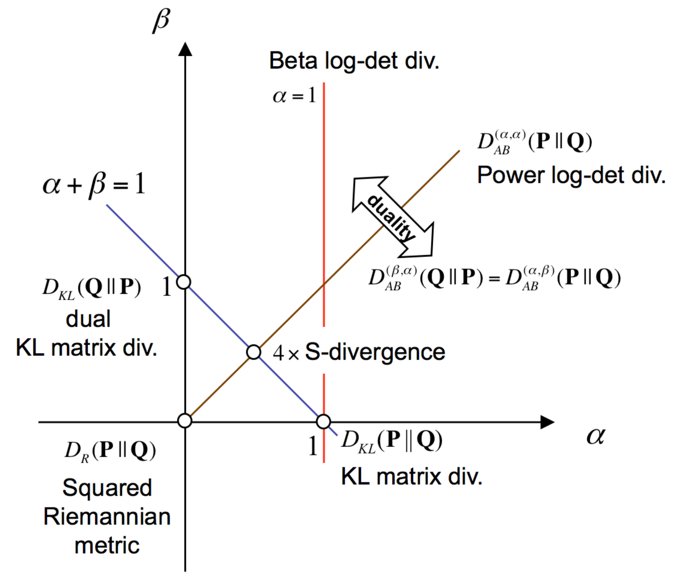
5. The Definition of the AB Log-Det Divergence

Henceforth, we will work on the multidimensional observation vectors $\mathit{x}={[x_1,\dots ,x_n]}^T\in {\mathbb{R}}^n$. In order to simplify the notation, the covariance matrices of the two classes are renamed as follows

$$\begin{array}{ccc}\hfill \mathbf{P}& \equiv & Cov(\mathit{x}|c_1),\hfill \end{array}$$

(36)

$$\begin{array}{ccc}\hfill \mathbf{Q}& \equiv & Cov(\mathit{x}|c_2).\hfill \end{array}$$

(37)

The AB log-det divergence is a directed divergence that evaluates the dissimilarity between two multidimensional covariance matrices. It was defined in [6] as

$$\begin{array}{ccc}\hfill D_{AB}^{(\alpha ,\beta )}(\mathbf{P}\parallel \mathbf{Q})& =& \frac{1}{\alpha \beta }log{\left|\frac{\alpha {({\mathbf{Q}}^{-\frac{1}{2}}\mathbf{P}{\mathbf{Q}}^{-\frac{1}{2}})}^{\beta }+\beta {({\mathbf{Q}}^{-\frac{1}{2}}\mathbf{P}{\mathbf{Q}}^{-\frac{1}{2}})}^{-\alpha }}{\alpha +\beta }\right|}_{+}\hfill \\ \hfill \\ & & \mathrm{for}\alpha \ne 0,\beta \ne 0,\alpha +\beta \ne 0,\hfill \end{array}$$

(38)

while, for the singular cases, its definition is given by

$$\begin{array}{ccc}\hfill D_{AB}^{(\alpha ,\beta )}(\mathbf{P}\parallel \mathbf{Q})& =& \left\{\begin{array}{cc}{\displaystyle \frac{1}{{\alpha }^2}\left[\mathrm{tr}\left({({\mathbf{Q}}^{\frac{1}{2}}{\mathbf{P}}^{-1}{\mathbf{Q}}^{\frac{1}{2}})}^{\alpha }-\mathbf{I}\right)-\alpha log|{\mathbf{Q}}^{\frac{1}{2}}{\mathbf{P}}^{-1}{\mathbf{Q}}^{\frac{1}{2}}|\right]}\hfill & \mathrm{for}\alpha \ne 0,\beta =0,\hfill \\ \\ {\displaystyle \frac{1}{{\beta }^2}\left[\mathrm{tr}\left({({\mathbf{Q}}^{-\frac{1}{2}}\mathbf{P}{\mathbf{Q}}^{-\frac{1}{2}})}^{\beta }-\mathbf{I}\right)-\beta log|{\mathbf{Q}}^{-\frac{1}{2}}\mathbf{P}{\mathbf{Q}}^{-\frac{1}{2}}|\right]}\hfill & \mathrm{for}\alpha =0,\beta \ne 0,\hfill \\ \\ {\displaystyle \frac{1}{{\alpha }^2}log{\left|{({\mathbf{Q}}^{-\frac{1}{2}}\mathbf{P}{\mathbf{Q}}^{-\frac{1}{2}})}^{\alpha }(\mathbf{I}+log{({\mathbf{Q}}^{-\frac{1}{2}}\mathbf{P}{\mathbf{Q}}^{-\frac{1}{2}})}^{-\alpha })\right|}_{+}}\hfill & \mathrm{for}\alpha =-\beta ,\hfill \\ \\ {\displaystyle \frac{1}{2}||log({\mathbf{Q}}^{\frac{1}{2}}{\mathbf{P}}^{-1}{\mathbf{Q}}^{\frac{1}{2}}){||}_F^2}\hfill & \mathrm{for}\alpha ,\beta =0.\hfill \end{array}\right.\hfill \end{array}$$

(39)

The divergence depends only on the eigenvalues $\mathbf{\Lambda }=\mathrm{diag}({\lambda }_1,\cdots ,{\lambda }_n)$ of the Symmetric Positive Definite (SPD) matrix ${\mathbf{Q}}^{-1/2}\mathbf{P}{\mathbf{Q}}^{-1/2}$, which also coincide with the eigenvalues of the matrix ${\mathbf{Q}}^{-1}\mathbf{P}$, although their eigenspaces differ. Given the eigenvalue decomposition

$$\begin{array}{c}\hfill {\mathbf{Q}}^{-\frac{1}{2}}\mathbf{P}{\mathbf{Q}}^{-\frac{1}{2}}={\mathbf{V}}_1\mathbf{\Lambda }{\mathbf{V}}_1^T,\end{array}$$

(40)

where ${\mathbf{V}}_1$ is the orthogonal matrix of eigenvectors, and $\mathbf{\Lambda }=\mathrm{diag}\{{\lambda }_1,{\lambda }_2,\dots ,{\lambda }_n\}$ is the diagonal matrix with positive eigenvalues ${\lambda }_i>0,i=1,2,\dots ,n$. One of the properties of the AB log-det divergence is that it is invariant under a common change of basis on its matrix arguments, i.e., an invertible congruence transformation. Since, with the help of this specific transformation, we have

$$\begin{array}{ccc}\hfill \mathbf{P}& \to & ({\mathbf{V}}_1^T{\mathbf{Q}}^{-\frac{1}{2}})\mathbf{P}{({\mathbf{V}}_1^T{\mathbf{Q}}^{-\frac{1}{2}})}^T=\mathbf{\Lambda },\hfill \end{array}$$

(41)

$$\begin{array}{ccc}\hfill \mathbf{Q}& \to & ({\mathbf{V}}_1^T{\mathbf{Q}}^{-\frac{1}{2}})\mathbf{Q}{({\mathbf{V}}_1^T{\mathbf{Q}}^{-\frac{1}{2}})}^T=\mathbf{I},\hfill \end{array}$$

(42)

it can be inferred that the divergence is separable (over the generalized eigenvalues of the matrix pencil $(\mathbf{P},\mathbf{Q})$) in a sum of marginal divergences that measure how far are each of the generalized eigenvalues from the unity, i.e.,

$$\begin{array}{c}\hfill D_{AB}^{(\alpha ,\beta )}(\mathbf{P}\parallel \mathbf{Q})=D_{AB}^{(\alpha ,\beta )}\left(\mathbf{\Lambda }\parallel {\mathbf{I}}_n\right)={\displaystyle \sum _{i=1}^n}{D}_{AB}^{(\alpha ,\beta )}({\lambda }_i\parallel 1).\end{array}$$

(43)

Hence,

$$\begin{array}{ccc}\hfill D_{AB}^{(\alpha ,\beta )}(\mathbf{P}\parallel \mathbf{Q})& =& \frac{1}{\alpha \beta }{\displaystyle \sum _{i=1}^n}log{\left|\frac{\alpha {\lambda }_i^{\beta }+\beta {\lambda }_i^{-\alpha }}{\alpha +\beta }\right|}_{+},\alpha ,\beta ,\alpha +\beta \ne 0.\hfill \end{array}$$

(44)

Similarly, for the singular cases, the divergence is

$$\begin{array}{ccc}\hfill D_{AB}^{(\alpha ,\beta )}(\mathbf{P}\parallel \mathbf{Q})& =& \left\{\begin{array}{cc}{\displaystyle \frac{1}{{\alpha }^2}\left[{\displaystyle \sum _{i=1}^n}\left({\lambda }_i^{-\alpha }-log({\lambda }_i^{-\alpha })\right)-n\right]}\hfill & \mathrm{for}\alpha \ne 0,\beta =0\hfill \\ \\ {\displaystyle \frac{1}{{\beta }^2}\left[{\displaystyle \sum _{i=1}^n}\left({\lambda }_i^{\beta }-log({\lambda }_i^{\beta })\right)-n\right]}\hfill & \mathrm{for}\alpha =0,\beta \ne 0\hfill \\ \\ {\displaystyle \frac{1}{{\alpha }^2}\left[{\displaystyle \sum _{i=1}^n}log{\left|\frac{{\lambda }_i^{\alpha }}{1+log{\lambda }_i^{\alpha }}\right|}_{+}\right]}\hfill & \mathrm{for}\alpha =-\beta \ne 0\hfill \\ \\ {\displaystyle \frac{1}{2}{\displaystyle \sum _{i=1}^n}{log}^2({\lambda }_i)}\hfill & \mathrm{for}\alpha ,\beta =0.\hfill \end{array}\right.\hfill \end{array}$$

(45)

This divergence compares two symmetric positive definite matrices and returns its dissimilarity, i.e., a positive value when they are non-coincident and $D_{AB}^{(\alpha ,\beta )}(\mathbf{P}\parallel \mathbf{Q})=0$ iff $\mathbf{P}=\mathbf{Q}$. As it can be observed in Figure 1 the AB log-det divergence generalizes several existing log-det matrix divergences, like: the Stein’s loss, the S-divergence, the Alpha and Beta log-det families of divergences and the geodesic distance between covariance matrices (the squared Riemannian metric), among others (see Table 1 in [6] for a comprehensive list).

5.1. A Tight Upper-Bound for the AB Log-Det Divergences

The divergence $D_{AB}^{(\alpha ,\beta )}(\mathbf{P}\parallel \mathbf{Q})$ depends on the generalized eigenvalues ${\lambda }_1,\cdots ,{\lambda }_n$ of the matrix pencil $(\mathbf{P},\mathbf{Q})$ which, for convenience, are assumed to have a simple spectrum (the eigenvalues are unique or non-coincident) and can be sorted in descending order

$$\begin{array}{c}\hfill {\lambda }_1>{\lambda }_2>\cdots >{\lambda }_n>0.\end{array}$$

(46)

In practice, the assumption is plausible because the real symmetric matrices with unique eigenvalues are known to form an open dense set in the space of all the real symmetric matrices [20].

Although the space of the observations is high-dimensional, most of the discriminative information between the two conditions is confined into a low-dimensional subspace. Thus, the spatial filter matrix $\mathbf{W}\in {\mathbb{R}}^{n\times p}$ is used to reduce the dimensionality of the samples from n to p with the linear compression transformation $\mathit{y}={\mathbf{W}}^T\mathit{x}\in {\mathbb{R}}^p$. It is shown in [6] that, after applying this compression to the arguments of the divergence, the resulting output covariance matrices ${\mathbf{W}}^T\mathbf{PW}$ and ${\mathbf{W}}^T\mathbf{QW}$ are more similar than in the original space, as shown in the below equation

$$\begin{array}{c}\hfill D_{AB}^{(\alpha ,\beta )}({\mathbf{W}}^T\mathbf{PW}\parallel {\mathbf{W}}^T\mathbf{QW})={\displaystyle \sum _{i=1}^p}{D}_{AB}^{(\alpha ,\beta )}({\mu }_i\parallel 1)\le {\displaystyle \sum _{i=1}^n}{D}_{AB}^{(\alpha ,\beta )}({\lambda }_i\parallel 1)=D_{AB}^{(\alpha ,\beta )}(\mathbf{P}\parallel \mathbf{Q}),\end{array}$$

(47)

where ${\mu }_1\ge \cdots \ge {\mu }_p>0$ are the generalized eigenvalues of the matrix pencil $({\mathbf{W}}^T\mathbf{PW},{\mathbf{W}}^T\mathbf{QW})$. However, this upper bound is loose for the case of interest (dimensionality reduction), i.e., when $p<n$. In Appendix A.1, the possible way to tighten the previous upper-bound with the following new proposal is shown

$$\begin{array}{c}\hfill D_{AB}^{(\alpha ,\beta )}({\mathbf{W}}^T\mathbf{PW}\parallel {\mathbf{W}}^T\mathbf{QW})\le {\displaystyle \sum _{i=1}^p}{D}_{AB}^{(\alpha ,\beta )}({\lambda }_{{\pi }_i}\parallel 1),\end{array}$$

(48)

where π defines the permutation of the indices $1,\dots ,n$ that sorts the divergence of the eigenvalues from the unity in descending order

$$\begin{array}{c}\hfill D_{AB}^{(\alpha ,\beta )}({\lambda }_{{\pi }_1}\parallel 1)\ge D_{AB}^{(\alpha ,\beta )}({\lambda }_{{\pi }_2}\parallel 1)\ge \cdots \ge D_{AB}^{(\alpha ,\beta )}({\lambda }_{{\pi }_n}\parallel 1).\end{array}$$

(49)

Moreover, the equality with the upper-bound is only obtained for those extraction matrices $\mathbf{W}$ that lie within the span of the p generalized eigenvectors of the matrix pencil $(\mathbf{P},\mathbf{Q})$ which are associated with the eigenvalues ${\lambda }_{{\pi }_1},\dots ,{\lambda }_{{\pi }_p}$ that maximize the divergence from unity in (49).

5.2. Relationship between the Generalized Eigenvalues and Eigenvectors of the Matrix Pencils $(\mathbf{P},\mathbf{Q})$ and $(p(c_1)\mathbf{P},Cov(\mathit{x}))$

We have seen in the previous section that the tight upper-bound of the divergence is attained by a subset of the generalized eigenvectors of the matrix pencil $(\mathbf{P},\mathbf{Q})$, whereas, the CSP solution in (24) depends on a subset of the generalized eigenvectors of another matrix pencil $(p(c_1)\mathbf{P},Cov(\mathit{x}))$. In this section we addresses the close relationship between both eigendecompositions. For this purpose, we recognize Λ as the matrix of eigenvalues of ${\mathbf{Q}}^{-1}\mathbf{P}$ and ${\mathbf{\Lambda }}^{(c_1)}$ as the matrix of eigenvalues of ${(Cov(\mathit{x}))}^{-1}p(c_1)\mathbf{P}$. Then, we write

$$\begin{array}{ccc}\hfill {(p(c_2)\mathbf{Q})}^{-1}(p(c_1)\mathbf{P})& =& {[{(Cov(\mathit{x}))}^{-1}(p(c_2)\mathbf{Q})]}^{-1}[{(Cov(\mathit{x}))}^{-1}(p(c_1)\mathbf{P})],\hfill \end{array}$$

(50)

and use the decomposition of $Cov(\mathit{x})$ in (4) to substitute $p(c_2)\mathbf{Q}=Cov(\mathit{x})-p(c_1)\mathbf{P}$ in the previous equation. In this way, we obtain

$$\begin{array}{ccc}\hfill {(p(c_2)\mathbf{Q})}^{-1}(p(c_1)\mathbf{P})& =& {[{\mathbf{I}}_n-{(Cov(\mathit{x}))}^{-1}(p(c_1)\mathbf{P})]}^{-1}[{(Cov(\mathit{x}))}^{-1}(p(c_1)\mathbf{P})].\hfill \end{array}$$

(51)

The matrix of eigenvectors $\mathbf{V}$ of ${\mathbf{Q}}^{-1}\mathbf{P}$ diagonalizes both sides of the previous equation

$$\begin{array}{}(52)& \hfill \mathbf{\Lambda }\frac{p(c_1)}{p(c_2)}& =& {\mathbf{V}}^{-1}\left[\frac{p(c_1)}{p(c_2)}{\mathbf{Q}}^{-1}\mathbf{P}\right]\mathbf{V}\hfill (53)& & =& ({\mathbf{V}}^{-1}{[{\mathbf{I}}_n-{(Cov(\mathit{x}))}^{-1}(p(c_1)\mathbf{P})]}^{-1}\mathbf{V})({\mathbf{V}}^{-1}[{(Cov(\mathit{x}))}^{-1}(p(c_1)\mathbf{P})]\mathbf{V})\hfill (54)& & =& {[{\mathbf{I}}_n-{\mathbf{V}}^{-1}{(Cov(\mathit{x}))}^{-1}(p(c_1)\mathbf{PV})]}^{-1}({\mathbf{V}}^{-1}[{(Cov(\mathit{x}))}^{-1}(p(c_1)\mathbf{P})]\mathbf{V})\hfill (55)& & =& {({\mathbf{I}}_n-{\mathbf{\Lambda }}^{(c_1)})}^{-1}{\mathbf{\Lambda }}^{(c_1)}.\hfill \end{array}$$

Hence, we have the explicit relationship between the two sets of eigenvalues

$$\begin{array}{c}\hfill {\lambda }_i\frac{p(c_1)}{p(c_2)}=\frac{{\lambda }_i^{(c_1)}}{1-{\lambda }_i^{(c_1)}}\equiv g({\lambda }_i^{(c_1)}),i=1,\dots ,n,\end{array}$$

(56)

where $g({\lambda }_i^{(c_1)})$, as can be seen in Figure 2, is a strictly monotonous ascending function over the domain of ${\lambda }_i^{(c_1)}\in (0,1)$. Moreover, the Equations (52)–(55) imply that the matrix $\mathbf{V}$ of generalized eigenvectors of the matrix pencil $(\mathbf{P},\mathbf{Q})$ exactly coincides with the matrix ${\mathbf{V}}^{(c_1)}$ of generalized eigenvectors of the other matrix pencil $(p(c_1)\mathbf{P},Cov(\mathit{x}))$.

5.3. Linking the Optimization of the Divergence and the CSP Solution

There is a link between the solutions of the CSP method and the solutions obtained with the optimization of the symmetric KL divergence between the class conditional covariances, which was studied in previous works [1,11,16]. This subsection shows that under the appropriate filter selection criteria the link also extends to the optimization of other divergences, like the AB log-det family of divergences.

We have previously assumed that generalized eigenvalues are ordered and can be regarded as non-equal. Therefore, we can cluster them in the following three sets of principal, inner and minor eigenvalues of the matrix pencil $(\mathbf{P},\mathbf{Q})$:

$$\begin{array}{c}\hfill \underset{k\mathrm{principal}\mathrm{eigenvalues}}{\underbrace{{\lambda }_1>\cdots >{\lambda }_k}}>\underset{\mathrm{inner}\mathrm{eigenvalues}}{\underbrace{{\lambda }_{k+1}>\cdots >{\lambda }_{n-(p-k)}}}>\underset{(p-k)\mathrm{minor}\mathrm{eigenvalues}}{\underbrace{{\lambda }_{n-(p-k)+1}>\cdots >{\lambda }_n}}.\end{array}$$

(57)

The following sequence of optimizations induces an alternative ordering of the generalized eigenvalues

$$\begin{array}{c}\hfill D_{AB}^{(\alpha ,\beta )}({\lambda }_{{\pi }_i}\parallel 1)=\underset{dim\{\mathcal{W}\}=n-i+1}{min}\underset{\mathit{w}\in \mathcal{W}}{max}{D}_{AB}^{(\alpha ,\beta )}({\mathit{w}}_i^T\mathbf{P}{\mathit{w}}_i\parallel {\mathit{w}}_i^T\mathbf{Q}{\mathit{w}}_i),i=1,\dots ,n,\end{array}$$

(58)

according to a permutation π that sorts their marginal divergences from 1 in descending order

$$\begin{array}{c}\hfill D_{AB}^{(\alpha ,\beta )}({\lambda }_{{\pi }_1}\parallel 1)\ge \cdots \ge D_{AB}^{(\alpha ,\beta )}({\lambda }_{{\pi }_p}\parallel 1)\ge D_{AB}^{(\alpha ,\beta )}({\lambda }_{{\pi }_{p+1}}\parallel 1)\cdots \ge D_{AB}^{(\alpha ,\beta )}({\lambda }_{{\pi }_n}\parallel 1).\end{array}$$

(59)

For building the matrix of spatial filters ${\mathbf{W}}_{Div}\equiv [{\mathit{w}}_1,{\mathit{w}}_2.....{\mathit{w}}_p]$, one possible selection policy is to retain only the p most discriminative spatial filters for the considered divergence optimization problem, i.e., those that solve (58) for $i=1,\dots ,p$. The filters consist in p eigenvectors (${\mathit{v}}_{{\pi }_i}$ with $i=1,\dots ,p$) of the matrix pencil $(\mathbf{P},\mathbf{Q})$ that are arranged according to the permutation π. From the one-to-one relationship that exists between the generalized eigenvalues and eigenvectors of the matrix pencils $(\mathbf{P},\mathbf{Q})$ and $(p(c_1)\mathbf{P},Cov(\mathit{x}))$ (see the previous subsection) the solution takes the following form

$$\begin{array}{}(60)& \hfill {\mathbf{W}}_{Div}& =& [{\mathit{v}}_{{\pi }_1},\dots ,{\mathit{v}}_{{\pi }_p}]\hfill (61)& & =& [{\mathit{v}}_{{\pi }_1}^{(c_1)},\dots ,{\mathit{v}}_{{\pi }_p}^{(c_1)}].\hfill \end{array}$$

This result tells us that the optimization of different divergences (in absence of other regularizing terms) only differs in the selection criteria for the spatial filters, which eventually determine the chosen subindices ${\pi }_1,\dots ,{\pi }_p$.

Now, the question of whether these spatial filters that solve the sequence of minimax divergence optimization problems

$$\begin{array}{c}\hfill \underset{dim\{\mathcal{W}\}=n-i+1}{min}\underset{\mathit{w}\in \mathcal{W}}{max}{D}_{AB}^{(\alpha ,\beta )}({\mathit{w}}_i^T\mathbf{P}{\mathit{w}}_i\parallel {\mathit{w}}_i^T\mathbf{Q}{\mathit{w}}_i),i=1,\dots ,p,\end{array}$$

(62)

essentially coincide (up to a possible permutation in the order of the spatial filters) with the spatial filters of the CSP solution in (63)

$$\begin{array}{c}\hfill {\mathbf{W}}_{CSP}=[\underset{k\mathrm{principal}\mathrm{eigenvectors}}{\underbrace{{\mathit{v}}_1^{(c_1)},\dots ,{\mathit{v}}_k^{(c_1)}}},\underset{p-k\mathrm{minor}\mathrm{eigenvectors}}{\underbrace{{\mathit{v}}_{n-(p-k)+1}^{(c_1)},\dots ,{\mathit{v}}_n^{(c_1)}}}],\end{array}$$

(63)

has a simple answer. The straightforward comparison between (61) and (63) reveals that both solutions should essentially coincide when the subindices ${\pi }_1,\dots ,{\pi }_p$ are a permutation of the integers $1,\dots ,k,n-(p-k)+1,\dots ,n$. Thus, the link between both techniques happens whenever CSP method adopts the filter selection policy of the divergence criterion in (59).

However, many of the CSP implementations find satisfactory to choose the number of spatial filters for each class a priori, respectively as k and $p-k$ (we will refer to this case as the original CSP filter selection policy), where k is close to $p/2$ in order to approximately balance the number of spatial filters for each class [13,21].

In general, the use of a divergence based selection policy does not ensure a balanced representation of the spatial filters for each of the classes. For instance, consider the synthetic but illustrative situation for $n=100$, where we wish to select $p=8$ spatial filters. If the generalized eigenvalues of the matrix pencil $(\mathbf{P},\mathbf{Q})$ are shifted towards to zero, for instance, equal to $\{10,0.99,0.98,\dots ,0.03,0.02,0.01\}$. In most cases, the solution ${\mathbf{W}}_{Div}$ will select as its columns: only $k=1$ principal eigenvectors and $p-k=7$ minor eigenvectors, an unbalanced choice.

In view of this potential limitation, an interesting question is whether it would be possible to modify the AB log-det divergence criterion so as to enforce that its solution essentially coincides with the one obtained by the CSP method with its original filter selection policy. We will show in the following that this requires only a suitable scaling $\kappa \in {\mathbb{R}}^{+}$ in one of the arguments of the divergence. Without loss of generality, we assume scaling in the second argument of the divergence. As it is shown in the Appendix A.2, there is a permutation ${\pi }^{\prime }$ of the indices of the spatial filters $1,\dots ,p$ that links the CSP solution in (24) with the optimization of the divergence

$$\begin{array}{c}\hfill {\mathit{w}}_{{\pi }_i^{\prime }}=arg\underset{dim\{\mathcal{W}\}=n-i+1}{min}\underset{\mathit{w}\in \mathcal{W}}{max}{D}_{AB}^{(\alpha ,\beta )}({\mathit{w}}_i^T\mathbf{P}{\mathit{w}}_i\parallel \kappa {\mathit{w}}_i^T\mathbf{Q}{\mathit{w}}_i),i=1,\dots ,p,\end{array}$$

(64)

for any given

$$\begin{array}{ccc}\hfill \kappa & \in & \left({\kappa }_{inf},{\kappa }_{sup}\right)\hfill \end{array}$$

(65)

with

$$\begin{array}{}(66)& \hfill {\kappa }_{inf}& \equiv & \mathcal{K}({\lambda }_{k+1},{\lambda }_{n-(p-k)+1})\hfill (67)& \hfill {\kappa }_{sup}& \equiv & \mathcal{K}({\lambda }_k,{\lambda }_{n-(p-k)})\hfill \end{array}$$

where the function

$$\begin{array}{ccc}\hfill \mathcal{K}(a,b)& =& \left\{\begin{array}{cc}{\displaystyle {\left(\frac{(a^{\beta }-b^{\beta })/\beta }{(a^{-\alpha }-b^{-\alpha })/(-\alpha )}\right)}^{\frac{1}{\alpha +\beta }}}& \mathrm{for}\alpha ,\beta ,\alpha +\beta \ne 0\hfill \\ \\ {\displaystyle {\left(\frac{log(a/b))}{(a^{-\alpha }-b^{-\alpha })/(-\alpha )}\right)}^{\frac{1}{\alpha }}}& \mathrm{for}\alpha \ne 0,\beta =0\hfill \\ \\ {\displaystyle {\left(\frac{(a^{\beta }-b^{\beta })/\beta }{log(a/b))}\right)}^{\frac{1}{\beta }}}& \mathrm{for}\alpha =0,\beta \ne 0\hfill \\ \\ {\displaystyle exp\left(\frac{a^{\alpha }log(e{b}^{\alpha })-b^{\alpha }log(e{a}^{\alpha })}{\alpha (a^{\alpha }-b^{\alpha })}\right)}& \mathrm{for}\alpha =-\beta \ne 0\hfill \\ \\ {\displaystyle \sqrt{ab}}& \mathrm{for}\alpha =\beta =0\hfill \end{array}\right.\hfill \end{array}$$

(68)

determines the value of the constant $\kappa =\mathcal{K}(a,b)\in \mathbb{R}$ that equalizes the value of the AB log-det divergences between any arbitrary $a,b\in \mathbb{R}$ constants (in the first argument) and κ (in the second argument), i.e.,

$$\begin{array}{c}\hfill D_{AB}^{(\alpha ,\beta )}(a\parallel \kappa )=D_{AB}^{(\alpha ,\beta )}(b\parallel \kappa ).\end{array}$$

(69)

Note that the only role of the scaling factor κ is to adjust the reference value in one of the arguments of the divergence to ensure the exact balance in the number of spatial filters that are specialized in each class. As it is shown in the Appendix A.2, this scaling factor prevents that the minimax solution for $i=1,\dots ,p$, could be attained by some eigenvectors associated with elements of the inner set of eigenvalues in (57), so the chosen subset of eigenvectors have to essentially coincide with the principal and minor eigenvectors that form the CSP solution in (63). In practice, a value of κ which is closer to unity and meets the required bounds can be obtained from the truncated choice

$$\begin{array}{ccc}\hfill {\kappa }_{★}& =& \left\{\begin{array}{cc}{\kappa }_{inf}+\epsilon & \mathrm{for}{\kappa }_{inf}\ge 1\hfill \\ 1& \mathrm{for}1\in ({\kappa }_{inf},{\kappa }_{sup})\hfill \\ {\kappa }_{sup}-\epsilon & \mathrm{for}{\kappa }_{sup}\le 1\hfill \end{array}\right.\hfill \end{array}$$

(70)

for an arbitrary small value of the constant $ϵ\ll {\kappa }_{sup}-{\kappa }_{inf}$.

6. The Gradient of the AB Log-Det Divergence

The AB log-det divergence between the conditional covariance of the outputs $\mathit{Y}={\mathbf{W}}^T\mathit{x}$ for each of the classes

$$\begin{array}{}(71)& \hfill f(\mathbf{W})& =& D_{AB}^{(\alpha ,\beta )}(Cov(\mathit{Y}|c_1)\parallel Cov(\mathit{Y}|c_2))\hfill (72)& & =& D_{AB}^{(\alpha ,\beta )}({\mathbf{W}}^T\mathbf{PW}\parallel {\mathbf{W}}^T\mathbf{QW}),\hfill \end{array}$$

is a function of the matrix $\mathbf{W}\in {\mathbb{R}}^{n\times p}$.

The optimization of this function with respect to $\mathbf{W}$ is non-trivial, so in this section, we show how the gradient of the AB log-det divergences can be derived. One may note that this is not only naturally interesting for the optimization that we would like to perform in this work, but it also contributes to pave the way for the potential practical use of the AB log-det divergence in other scenarios and applications.

As we have shown previously, the divergence is separable

$$\begin{array}{ccc}\hfill D_{AB}^{(\alpha ,\beta )}({\mathbf{W}}^T\mathbf{PW}\parallel {\mathbf{W}}^T\mathbf{QW})& =& D_{AB}^{(\alpha ,\beta )}(\mathbf{M}\parallel {\mathbf{I}}_p)={\displaystyle \sum _{i=1}^p}{D}_{AB}^{(\alpha ,\beta )}({\mu }_i(\mathbf{W})\parallel 1)\hfill \end{array}$$

(73)

over the eigenvalues of the matrix

$$\begin{array}{}(74)& \hfill \mathbf{M}& =& {({\mathbf{W}}^T\mathbf{QW})}^{-\frac{1}{2}}{\mathbf{W}}^T\mathbf{P}\mathbf{W}{({\mathbf{W}}^T\mathbf{QW})}^{-\frac{1}{2}}\hfill (75)& & =& \mathbf{U}\mathrm{diag}\{{\mu }_1,\cdots ,{\mu }_n\}{\mathbf{U}}^T\hfill \end{array}$$

where $\mathrm{diag}\{{\mu }_1,\cdots ,{\mu }_p\}$ and $\mathbf{U}=[{\mathit{u}}_1,\cdots ,{\mathit{u}}_p]$, respectively denote the matrices of eigenvalues and eigenvectors of $\mathbf{M}$, which are functions of the matrix $\mathbf{W}$.

The differential of $f(\mathbf{W})$ can be expressed as

$$\begin{array}{ccc}\hfill df(\mathbf{W})& =& \mathrm{tr}\left\{d{\mathbf{W}}^T\frac{\partial f(\mathbf{W})}{\partial \mathbf{W}}\right\}\hfill \end{array}$$

(76)

where

$$\begin{array}{c}\hfill \frac{\partial f(\mathbf{W})}{\partial \mathbf{W}}={\left[\frac{\partial f(\mathbf{W})}{\partial W_{ij}}\right]}_{ij}\in {\mathbb{R}}^{n\times p}\end{array}$$

(77)

denotes the gradient of the function. The divergence directly depends on the generalized eigenvalues, which in turn depend on the matrix $\mathbf{W}$. The suitable tool to obtain the gradient of this composition of functions is the chain rule, which can be written as

$$\begin{array}{ccc}\hfill \frac{\partial f(\mathbf{W})}{\partial \mathbf{W}}& =& {\displaystyle \sum _{i=1}^p}\frac{\partial {\mu }_i}{\partial \mathbf{W}}\frac{\partial f(\mathbf{W})}{\partial {\mu }_i}.\hfill \end{array}$$

(78)

So, the gradient can be evaluated after finding $\frac{\partial f(\mathbf{W})}{\partial {\mu }_i}$ and $\frac{\partial {\mu }_i}{\partial \mathbf{W}}$.

Since the divergence is a separable function of the generalized eigenvalues, the first term is easier to obtain,

$$\begin{array}{c}\hfill \frac{\partial f(\mathbf{W})}{\partial {\mu }_i}=\frac{\partial D_{AB}^{(\alpha ,\beta )}({\mu }_i\parallel 1)}{\partial {\mu }_i}=\left\{\begin{array}{cc}{\displaystyle \frac{{\mu }_i^{\beta -1}-{\mu }_i^{-\alpha -1}}{\alpha {\mu }_i^{\beta }+\beta {\mu }_i^{-\alpha }}=\frac{{\mu }_i^{\alpha +\beta }-1}{{\mu }_i(\alpha {\mu }_i^{\alpha +\beta }+\beta )}}\hfill & \mathrm{for}\alpha +\beta \ne 0\hfill \\ \\ {\displaystyle \frac{log{\mu }_i}{{\mu }_i(1+\alpha log{\mu }_i)}}\hfill & \mathrm{for}\alpha +\beta =0.\hfill \end{array}\right.\end{array}$$

(79)

Obtaining the second term $\frac{\partial {\mu }_i}{\partial \mathbf{W}}$ is not so easy and requires to employ our previous plausible assumption that the generalized eigenvalues have a simple spectrum. Under this condition, the Hadamard first variation formula can be used to write the differential of the eigenvalues as

$$\begin{array}{c}\hfill d{\mu }_i={\mathit{u}}_i^{T}d\mathbf{M}{\mathit{u}}_i,\end{array}$$

(80)

where ${\mathit{u}}_i$ denotes the normalized eigenvector ($\parallel {\mathit{u}}_i{\parallel }_2=1$) corresponding to each eigenvalue ${\mu }_i$.

With the help of the product rule for differentials, we obtain

$$\begin{array}{ccc}\hfill d\mathbf{M}& =& d{({\mathbf{W}}^T\mathbf{QW})}^{-\frac{1}{2}}{({\mathbf{W}}^T\mathbf{QW})}^{\frac{1}{2}}\mathbf{M}+\hfill \\ & & \mathbf{M}{({\mathbf{W}}^T\mathbf{QW})}^{\frac{1}{2}}d{({\mathbf{W}}^T\mathbf{QW})}^{-\frac{1}{2}}+\hfill \\ & & {({\mathbf{W}}^T\mathbf{QW})}^{-\frac{1}{2}}(d{\mathbf{W}}^T\mathbf{PW}+{\mathbf{W}}^T\mathbf{P}d\mathbf{W}){({\mathbf{W}}^T\mathbf{QW})}^{-\frac{1}{2}}.\hfill \end{array}$$

(81)

As we show in the Appendix A.3, it can be simplified as follows

$$\begin{array}{}(82)& \hfill d{({\mathbf{W}}^T\mathbf{QW})}^{-\frac{1}{2}}{({\mathbf{W}}^T\mathbf{QW})}^{\frac{1}{2}}& =& -\frac{1}{2}{({\mathbf{W}}^T\mathbf{QW})}^{-\frac{1}{2}}d({\mathbf{W}}^T\mathbf{QW}){({\mathbf{W}}^T\mathbf{QW})}^{-\frac{1}{2}}\hfill (83)& & =& -\frac{1}{2}{({\mathbf{W}}^T\mathbf{QW})}^{-\frac{1}{2}}(d{\mathbf{W}}^T\mathbf{QW}+{\mathbf{W}}^T\mathbf{Q}d\mathbf{W}){({\mathbf{W}}^T\mathbf{QW})}^{-\frac{1}{2}}\hfill \end{array}$$

hence

$$\begin{array}{ccc}\hfill d\mathbf{M}& =& -\frac{1}{2}{({\mathbf{W}}^T\mathbf{QW})}^{-\frac{1}{2}}(d{\mathbf{W}}^T\mathbf{QW}+{\mathbf{W}}^T\mathbf{Q}d\mathbf{W}){({\mathbf{W}}^T\mathbf{QW})}^{-\frac{1}{2}}\mathbf{M}\hfill \\ & & -\frac{1}{2}{\left[{({\mathbf{W}}^T\mathbf{QW})}^{-\frac{1}{2}}(d{\mathbf{W}}^T\mathbf{QW}+{\mathbf{W}}^T\mathbf{Q}d\mathbf{W}){({\mathbf{W}}^T\mathbf{QW})}^{-\frac{1}{2}}\mathbf{M}\right]}^T\hfill \\ & & +{({\mathbf{W}}^T\mathbf{QW})}^{-\frac{1}{2}}(d{\mathbf{W}}^T\mathbf{PW}+{\mathbf{W}}^T\mathbf{P}d\mathbf{W}){({\mathbf{W}}^T\mathbf{QW})}^{-\frac{1}{2}}.\hfill \end{array}$$

(84)

Thus, after substituting (84) in (80) and using the invariance of the trace under transpositions ($\mathrm{tr}\{\mathbf{A}\}=\mathrm{tr}\{{\mathbf{A}}^T\}$) and the cyclic shifts ($\mathrm{tr}\{\mathbf{A}\mathbf{B}\}=\mathrm{tr}\{\mathbf{B}\mathbf{A}\}$), the following values are obtained

$$\begin{array}{}(85)& \hfill d{\mu }_i& =& {\mathit{u}}_i^{T}d\mathbf{M}{\mathit{u}}_i\hfill (86)& & =& \mathrm{tr}\left\{{\mathit{u}}_i^{T}d\mathbf{M}{\mathit{u}}_i\right\}\hfill & & =& -\frac{1}{2}\mathrm{tr}\left\{{\mathit{u}}_i^T{({\mathbf{W}}^T\mathbf{QW})}^{-\frac{1}{2}}(d{\mathbf{W}}^T\mathbf{QW}+{\mathbf{W}}^T\mathbf{Q}d\mathbf{W}){({\mathbf{W}}^T\mathbf{QW})}^{-\frac{1}{2}}\mathbf{M}{\mathit{u}}_i\right\}\hfill & & & -\frac{1}{2}\mathrm{tr}\left\{{\mathit{u}}_i^T{\left[{({\mathbf{W}}^T\mathbf{QW})}^{-\frac{1}{2}}(d{\mathbf{W}}^T\mathbf{QW}+{\mathbf{W}}^T\mathbf{Q}d\mathbf{W}){({\mathbf{W}}^T\mathbf{QW})}^{-\frac{1}{2}}\mathbf{M}\right]}^T{\mathit{u}}_i\right\}\hfill (87)& & & +\mathrm{tr}\left\{{\mathit{u}}_i^T{({\mathbf{W}}^T\mathbf{QW})}^{-\frac{1}{2}}(d{\mathbf{W}}^T\mathbf{PW}+{\mathbf{W}}^T\mathbf{P}d\mathbf{W}){({\mathbf{W}}^T\mathbf{QW})}^{-\frac{1}{2}}{\mathit{u}}_i\right\}\hfill & & =& -2\mathrm{tr}\left\{d{\mathbf{W}}^T\mathbf{QW}{({\mathbf{W}}^T\mathbf{QW})}^{-\frac{1}{2}}\mathbf{M}{\mathit{u}}_i{\mathit{u}}_i^T{({\mathbf{W}}^T\mathbf{QW})}^{-\frac{1}{2}}\right\}\hfill (88)& & & +2\mathrm{tr}\left\{d{\mathbf{W}}^T\mathbf{PW}{({\mathbf{W}}^T\mathbf{QW})}^{-\frac{1}{2}}{\mathit{u}}_i{\mathit{u}}_i^T{({\mathbf{W}}^T\mathbf{QW})}^{-\frac{1}{2}}\right\}.\hfill \end{array}$$

At this point, we can use the identity for the differential

$$\begin{array}{ccc}\hfill d{\mu }_i& =& \mathrm{tr}\left\{d{\mathbf{W}}^T\frac{\partial {\mu }_i}{\partial \mathbf{W}}\right\}\hfill \end{array}$$

(89)

in (88) to identify the second desired term

$$\begin{array}{c}\hfill \frac{\partial {\mu }_i}{\partial \mathbf{W}}=-2\mathbf{QW}{({\mathbf{W}}^T\mathbf{QW})}^{-\frac{1}{2}}\mathbf{M}{\mathit{u}}_i{\mathit{u}}_i^T{({\mathbf{W}}^T\mathbf{QW})}^{-\frac{1}{2}}+2\mathbf{P}\mathbf{W}{({\mathbf{W}}^T\mathbf{QW})}^{-\frac{1}{2}}{\mathit{u}}_i{\mathit{u}}_i^T{({\mathbf{W}}^T\mathbf{QW})}^{-\frac{1}{2}}.\end{array}$$

(90)

Substituting the expressions (79) and (90) in (78), we obtain

$$\begin{array}{ccc}\hfill \frac{\partial f(\mathbf{W})}{\partial \mathbf{W}}& =& {\displaystyle \sum _{i=1}^p}\frac{\partial {\mu }_i}{\partial \mathbf{W}}\frac{\partial D_{AB}^{(\alpha ,\beta )}({\mu }_i\parallel 1)}{\partial {\mu }_i}\hfill \\ & =& -2\mathbf{QW}{({\mathbf{W}}^T\mathbf{QW})}^{-\frac{1}{2}}\mathbf{M}\mathbf{Z}{({\mathbf{W}}^T\mathbf{QW})}^{-\frac{1}{2}}+2\mathbf{P}\mathbf{W}{({\mathbf{W}}^T\mathbf{QW})}^{-\frac{1}{2}}\mathbf{Z}{({\mathbf{W}}^T\mathbf{QW})}^{-\frac{1}{2}}\hfill \end{array}$$

(91)

where, for convenience, the matrix is defined as following

$$\begin{array}{}(92)& \hfill \mathbf{Z}& =& {\displaystyle \sum _{i=1}^p}{\mathit{u}}_i\frac{\partial D_{AB}^{(\alpha ,\beta )}({\mu }_i\parallel 1)}{\partial {\mu }_i}{\mathit{u}}_i^T\hfill (93)& & =& \mathbf{U}\mathrm{diag}\left\{\frac{\partial D_{AB}^{(\alpha ,\beta )}({\mu }_1\parallel 1)}{\partial {\mu }_1},\dots ,\frac{\partial D_{AB}^{(\alpha ,\beta )}({\mu }_p\parallel 1)}{\partial {\mu }_p}\right\}{\mathbf{U}}^T.\hfill \end{array}$$

The matrix $\mathbf{Z}$ can also be represented directly in terms of the matrix $\mathbf{M}$ (which we have defined previously in Equation (74)) as

$$\begin{array}{ccc}\hfill \mathbf{Z}& =& \left\{\begin{array}{cc}{\displaystyle {\mathbf{M}}^{-1}{(\alpha {\mathbf{M}}^{\alpha +\beta }+\beta \mathbf{I})}^{-1}({\mathbf{M}}^{\alpha +\beta }-\mathbf{I})}\hfill & \mathrm{for}\alpha +\beta \ne 0\hfill \\ \\ {\displaystyle {\mathbf{M}}^{-1}{({(log\mathbf{M})}^{-1}+\alpha \mathbf{I})}^{-1}}\hfill & \mathrm{for}\alpha +\beta =0\hfill \end{array}\right.\hfill \end{array}$$

(94)

where $log(·)$ for matrix arguments denotes the matrix logarithm functional. After the grouping of common terms in (91) we obtain the final gradient expression, which is given by

$$\begin{array}{ccc}\hfill \frac{\partial f(\mathbf{W})}{\partial \mathbf{W}}& =& 2[\mathbf{PW}-\mathbf{QW}{({\mathbf{W}}^T\mathbf{QW})}^{-1}({\mathbf{W}}^T\mathbf{PW})]{({\mathbf{W}}^T\mathbf{QW})}^{-\frac{1}{2}}\mathbf{Z}{({\mathbf{W}}^T\mathbf{QW})}^{-\frac{1}{2}}.\hfill \end{array}$$

(95)

6.1. Validation of Equation (95) with the Gradient of the KL Divergence

The Kullback–Leibler (KL) divergence between the Gaussian densities $p(\mathit{x}|c_2)$ and the $p(\mathit{x}|c_1)$, of zero mean and the respective covariance matrices $Cov(\mathit{Y}|c_1)$ and $Cov(\mathit{Y}|c_2)$, is given by

$$\begin{array}{ccc}\hfill Di{v}_{KL}(p(\mathit{x}|c_2)\parallel p(\mathit{x}|c_1))& =& \int p(\mathit{x}|c_2)log\frac{p(\mathit{x}|c_2)}{p(\mathit{x}|c_1)}d\mathit{x}\hfill \\ & =& \frac{1}{2}log|Cov(\mathit{Y}|c_1)|-\frac{1}{2}log|Cov(\mathit{Y}|c_2)|+\frac{1}{2}\mathrm{tr}\{Co{v}^{-1}(\mathit{Y}|c_1)Cov(\mathit{Y}|c_2)-{\mathbf{I}}_p\}.\hfill \end{array}$$

(96)

Since this divergence only involves trace and log-det operators, as it is shown in the Appendix A.4, its gradient with respect to $\mathbf{W}$, i.e.,

$$\begin{array}{ccc}\hfill \frac{\partial }{\partial \mathbf{W}}Di{v}_{KL}(p(\mathit{x}|c_2)\parallel p(\mathit{x}|c_1))& =& -\mathbf{QW}{({\mathbf{W}}^T\mathbf{QW})}^{-1}+\mathbf{PW}{({\mathbf{W}}^T\mathbf{PW})}^{-1}+\mathbf{QW}{({\mathbf{W}}^T\mathbf{PW})}^{-1}\hfill \\ & & +\mathbf{PW}{({\mathbf{W}}^T\mathbf{PW})}^{-1}{({\mathbf{W}}^T\mathbf{QW})}^{-1}{({\mathbf{W}}^T\mathbf{PW})}^{-1},\hfill \end{array}$$

(97)

is relatively easy to obtain. Then, we can use the fact that the KL divergence is proportional to the AB log-det divergence between the class conditional covariance matrices, as long as the conditional covariance matrices appear in the AB log-det divergence interchanged in position with respect to class conditional density arguments of the KL divergence. So for the specific case of $\alpha =1$ and $\beta =0$, i.e.,

$$\begin{array}{ccc}\hfill D_{AB}^{(1,0)}(Cov(\mathit{Y}|c_1)\parallel Cov(\mathit{Y}|c_2))& =& 2Di{v}_{KL}(p(\mathit{x}|c_2)\parallel p(\mathit{x}|c_1)),\hfill \end{array}$$

(98)

to test whether there is coherence between the obtained gradient formula in (95) and twice the gradient of the KL divergence that was independently obtained in the Appendix A.4. For this purpose, in the specific case of $\alpha =1$ and $\beta =0$, from (94) the following auxiliary matrices are evaluated

$$\begin{array}{}(99)& \hfill \mathbf{Z}& =& {\mathbf{M}}^{-1}({\mathbf{I}}_p-{\mathbf{M}}^{-1})\hfill (100)& \hfill {({\mathbf{W}}^T\mathbf{QW})}^{-\frac{1}{2}}\mathbf{Z}{({\mathbf{W}}^T\mathbf{QW})}^{-\frac{1}{2}}& =& {({\mathbf{W}}^T\mathbf{PW})}^{-1}-{({\mathbf{W}}^T\mathbf{PW})}^{-1}({\mathbf{W}}^T\mathbf{QW}){({\mathbf{W}}^T\mathbf{PW})}^{-1}\hfill \end{array}$$

and are substituted in the expression of the gradient of the AB log-det divergence (95). After the following straightforward simplifications,

$$\begin{array}{}& \hfill \frac{\partial }{\partial \mathbf{W}}{D}_{AB}^{(1,0)}(Cov(\mathit{Y}|c_1)\parallel Cov(\mathit{Y}|c_2))& =& 2[\mathbf{PW}-\mathbf{QW}{({\mathbf{W}}^T\mathbf{QW})}^{-1}({\mathbf{W}}^T\mathbf{PW})]\hfill (101)& & & \times [{({\mathbf{W}}^T\mathbf{QW})}^{-\frac{1}{2}}\mathbf{Z}{({\mathbf{W}}^T\mathbf{QW})}^{-\frac{1}{2}}]\hfill & & =& 2[-\mathbf{QW}{({\mathbf{W}}^T\mathbf{QW})}^{-1}({\mathbf{W}}^T\mathbf{PW})+\mathbf{PW}]\hfill (102)& & & \times [{({\mathbf{W}}^T\mathbf{PW})}^{-1}-{({\mathbf{W}}^T\mathbf{PW})}^{-1}({\mathbf{W}}^T\mathbf{QW}){({\mathbf{W}}^T\mathbf{PW})}^{-1}]\hfill & & =& 2\left[-\mathbf{QW}{({\mathbf{W}}^T\mathbf{QW})}^{-1}+\mathbf{PW}{({\mathbf{W}}^T\mathbf{P}\mathbf{W})}^{-1}+\mathbf{QW}{({\mathbf{W}}^T\mathbf{P}\mathbf{W})}^{-1}\right.\hfill (103)& & & \left.+\mathbf{PW}{({\mathbf{W}}^T\mathbf{P}\mathbf{W})}^{-1}{({\mathbf{W}}^T\mathbf{QW})}^{-1}{({\mathbf{W}}^T\mathbf{P}\mathbf{W})}^{-1}\right]\hfill (104)& & =& 2\frac{\partial }{\partial \mathbf{W}}Di{v}_{KL}(p(\mathit{x}|c_2)\parallel p(\mathit{x}|c_1)).\hfill \end{array}$$

the proportionality between the gradient of $D_{AB}^{(1,0)}(Cov(\mathit{Y}|c_1)\parallel Cov(\mathit{Y}|c_2))$ and the gradient of the KL divergence in (97) is confirmed.

6.2. Validation of Equation (95) with the Gradient of the AG Divergence

The Alpha–Gamma divergence between the Gaussian densities $p(\mathit{x}|c_2)$ and $p(\mathit{x}|c_1)$, of zero mean and with respective covariance matrices $Cov(\mathit{Y}|c_1)={\mathbf{W}}^T\mathbf{PW}$ and $Cov(\mathit{Y}|c_2)={\mathbf{W}}^T\mathbf{QW}$, is equal to

$$\begin{array}{}(105)& \hfill Di{v}_{AG}^{(\alpha ,\beta )}\left(p(y_i|c_2)\parallel p(y_i|c_1)\right)& \equiv & \frac{1}{\alpha \beta }log\frac{{\left({\displaystyle {\int }_{\mathbf{\Omega }}p(y_i|c_1)d{y}_i}\right)}^{\beta }{\left({\displaystyle \int p(y_i|c_2)d{y}_i}\right)}^{\alpha }}{{\displaystyle \int p^{\beta }(y_i|c_1)p^{\alpha }(y_i|c_2)d{y}_i}}\hfill & & =& \frac{1}{2\alpha \beta }log|{\mathbf{W}}^T(\alpha \mathbf{P}+\beta \mathbf{Q})\mathbf{W}|-\frac{1}{2\beta }log|{\mathbf{W}}^T\mathbf{PW}|-\frac{1}{2\alpha }log|{\mathbf{W}}^T\mathbf{QW}|\hfill (106)& & & \mathrm{for}\alpha >0,\beta >0,\alpha +\beta =1.\hfill \end{array}$$

Due to the constraint $\alpha +\beta =1$, we assume that β is determined by α, i.e., $\beta =1-\alpha$ along this subsection. Since

$$\begin{array}{ccc}\hfill {\nabla }_{\mathbf{W}}log|({\mathbf{W}}^T\mathbf{PW})|& =& 2\mathbf{PW}{({\mathbf{W}}^T\mathbf{PW})}^{-1},\hfill \end{array}$$

(107)

the gradient of the AG divergence with respect to $\mathbf{W}$ is given by

$$\begin{array}{ccc}\hfill \frac{\partial }{\partial \mathbf{W}}Di{v}_{AG}^{(\alpha ,\beta )}(p(\mathit{x}|c_2)\parallel p(\mathit{x}|c_1))& =& \frac{2}{2\alpha \beta }(\alpha \mathbf{P}+\beta \mathbf{Q})\mathbf{W}{\left({\mathbf{W}}^T(\alpha \mathbf{P}+\beta \mathbf{Q})\mathbf{W}\right)}^{-1}\hfill \\ & & -\frac{2}{2\alpha }\mathbf{QW}{({\mathbf{W}}^T\mathbf{QW})}^{-1}-\frac{2}{2\beta }\mathbf{PW}{({\mathbf{W}}^T\mathbf{PW})}^{-1}\hfill \\ & =& -\frac{1}{\beta }\mathbf{PW}[{({\mathbf{W}}^T\mathbf{P}\mathbf{W})}^{-1}-{\left({\mathbf{W}}^T(\alpha \mathbf{P}+\beta \mathbf{Q})\mathbf{W}\right)}^{-1}]\hfill \\ & & -\frac{1}{\alpha }\mathbf{QW}[{({\mathbf{W}}^T\mathbf{QW})}^{-1}-{\left({\mathbf{W}}^T(\alpha \mathbf{P}+\beta \mathbf{Q})\mathbf{W}\right)}^{-1}].\hfill \end{array}$$

(108)

Then, we can use the equivalence between the AG divergence and the AB log-det divergence between the class conditional covariance matrices

$$\begin{array}{ccc}\hfill D_{AB}^{(\alpha ,\beta )}(Cov(\mathit{Y}|c_1)\parallel Cov(\mathit{Y}|c_2))& =& 2Di{v}_{AG}^{(\alpha ,\beta )}\left(p(y_i|c_2)\parallel p(y_i|c_1)\right),\hfill \end{array}$$

(109)

which is valid for the specific case of $\alpha +\beta =1$ and $\alpha ,\beta >0$, to also test the coherence between the obtained gradient formula in (95) and twice the gradient of the AG divergence. For $\alpha +\beta =1$, the auxiliary matrices in the definition of the gradient are

$$\begin{array}{ccc}\hfill \mathbf{Z}& =& {(\alpha \mathbf{M}+\beta \mathbf{I})}^{-1}[{\mathbf{M}}^{-1}(\mathbf{M}-\mathbf{I})]={(\alpha \mathbf{M}+\beta \mathbf{I})}^{-1}-{(\alpha {\mathbf{M}}^2+\beta \mathbf{M})}^{-1}\hfill \end{array}$$

(110)

and

$$\begin{array}{}& \hfill {({\mathbf{W}}^T\mathbf{QW})}^{-\frac{1}{2}}\mathbf{Z}{({\mathbf{W}}^T\mathbf{QW})}^{-\frac{1}{2}}& =& {(\alpha {({\mathbf{W}}^T\mathbf{QW})}^{\frac{1}{2}}\mathbf{M}{({\mathbf{W}}^T\mathbf{QW})}^{\frac{1}{2}}+\beta {\mathbf{W}}^T\mathbf{QW})}^{-1}\hfill & & & -(\alpha {({\mathbf{W}}^T\mathbf{QW})}^{\frac{1}{2}}\mathbf{M}{({\mathbf{W}}^T\mathbf{QW})}^{\frac{1}{2}}{({\mathbf{W}}^T\mathbf{QW})}^{-1}{({\mathbf{W}}^T\mathbf{QW})}^{\frac{1}{2}}\mathbf{M}{({\mathbf{W}}^T\mathbf{QW})}^{\frac{1}{2}}\hfill (111)& & & +\beta {({\mathbf{W}}^T\mathbf{QW})}^{\frac{1}{2}}\mathbf{M}{({\mathbf{W}}^T\mathbf{QW})}^{\frac{1}{2}}{)}^{-1}\hfill (112)& & =& [\mathbf{I}-{({\mathbf{W}}^T\mathbf{P}\mathbf{W})}^{-1}({\mathbf{W}}^T\mathbf{QW})]{({\mathbf{W}}^T(\alpha \mathbf{P}+\beta \mathbf{Q})\mathbf{W})}^{-1}.\hfill \end{array}$$

After substituting this last expression in the gradient of the AB log-det divergence (95), we obtain

$$\begin{array}{ccc}\hfill \frac{\partial }{\partial \mathbf{W}}{D}_{AB}^{(\alpha ,\beta )}(Cov(\mathit{Y}|c_1)\parallel Cov(\mathit{Y}|c_2))& & \hfill \\ & =& 2[\mathbf{PW}-\mathbf{QW}{({\mathbf{W}}^T\mathbf{QW})}^{-1}({\mathbf{W}}^T\mathbf{PW})]{({\mathbf{W}}^T\mathbf{QW})}^{-\frac{1}{2}}\mathbf{Z}{({\mathbf{W}}^T\mathbf{QW})}^{-\frac{1}{2}}\hfill \\ & =& +2(\mathbf{PW}+\mathbf{QW}){({\mathbf{W}}^T(\alpha \mathbf{P}+\beta \mathbf{Q})\mathbf{W})}^{-1}\hfill \\ & & -\frac{2}{\beta }\alpha \mathbf{PW}{[({\mathbf{W}}^T\alpha \mathbf{P}\mathbf{W})+({\mathbf{W}}^T\alpha \mathbf{P}\mathbf{W}){({\mathbf{W}}^T\beta \mathbf{QW})}^{-1}({\mathbf{W}}^T\alpha \mathbf{P}\mathbf{W})]}^{-1}\hfill \\ & & -\frac{2}{\alpha }\beta \mathbf{QW}{[({\mathbf{W}}^T\beta \mathbf{QW})+({\mathbf{W}}^T\beta \mathbf{QW}){({\mathbf{W}}^T\alpha \mathbf{P}\mathbf{W})}^{-1}({\mathbf{W}}^T\beta \mathbf{QW})]}^{-1}.\hfill \end{array}$$

(113)

With the help of the particular form of the Woodbury identity for the matrix inverse

$$\begin{array}{c}\hfill {[\mathbf{A}+\mathbf{A}{\mathbf{B}}^{-1}\mathbf{A}]}^{-1}={\mathbf{A}}^{-1}-{(\mathbf{A}+\mathbf{B})}^{-1}\end{array}$$

(114)

we simplify the terms within the brackets. Finally, we use the fact that $\alpha +\beta =1$ to confirm the proportionality with the gradient of the AG divergence given in (108),

$$\begin{array}{}& \hfill \frac{\partial }{\partial \mathbf{W}}{D}_{AB}^{(\alpha ,\beta )}(Cov(\mathit{Y}|c_1)\parallel Cov(\mathit{Y}|c_2))& =& +2(\mathbf{PW}+\mathbf{QW}){({\mathbf{W}}^T(\alpha \mathbf{P}+\beta \mathbf{Q})\mathbf{W})}^{-1}\hfill & & & -\frac{2}{\beta }\alpha \mathbf{PW}[{({\mathbf{W}}^T\alpha \mathbf{P}\mathbf{W})}^{-1}-{({\mathbf{W}}^T(\alpha \mathbf{P}+\beta \mathbf{Q})\mathbf{W})}^{-1}]\hfill (115)& & & -\frac{2}{\alpha }\beta \mathbf{QW}[{({\mathbf{W}}^T\beta \mathbf{QW})}^{-1}-{({\mathbf{W}}^T(\alpha \mathbf{P}+\beta \mathbf{Q})\mathbf{W})}^{-1}]\hfill & & =& +2(\mathbf{PW}+\mathbf{QW}){({\mathbf{W}}^T(\alpha \mathbf{P}+\beta \mathbf{Q})\mathbf{W})}^{-1}\hfill & & & -\frac{2}{\beta }\mathbf{PW}[{({\mathbf{W}}^T\mathbf{P}\mathbf{W})}^{-1}-\alpha {({\mathbf{W}}^T(\alpha \mathbf{P}+\beta \mathbf{Q})\mathbf{W})}^{-1}]\hfill (116)& & & -\frac{2}{\alpha }\mathbf{QW}[{({\mathbf{W}}^T\mathbf{QW})}^{-1}-\beta {({\mathbf{W}}^T(\alpha \mathbf{P}+\beta \mathbf{Q})\mathbf{W})}^{-1}]\hfill & & =& +2((1+\frac{\alpha }{\beta })\mathbf{PW}+(1+\frac{\beta }{\alpha })\mathbf{QW}){({\mathbf{W}}^T(\alpha \mathbf{P}+\beta \mathbf{Q})\mathbf{W})}^{-1}\hfill (117)& & & -\frac{2}{\beta }\mathbf{PW}{({\mathbf{W}}^T\mathbf{PW})}^{-1}-\frac{2}{\alpha }\mathbf{QW}{({\mathbf{W}}^T\mathbf{QW})}^{-1}\hfill & & =& +2(\frac{1}{\beta }\mathbf{PW}+\frac{1}{\alpha }\mathbf{QW}){({\mathbf{W}}^T(\alpha \mathbf{P}+\beta \mathbf{Q})\mathbf{W})}^{-1}\hfill (118)& & & -\frac{2}{\beta }\mathbf{PW}{({\mathbf{W}}^T\mathbf{PW})}^{-1}-\frac{2}{\alpha }\mathbf{QW}{({\mathbf{W}}^T\mathbf{QW})}^{-1}\hfill (119)& & =& 2\frac{\partial }{\partial \mathbf{W}}Di{v}_{AG}^{(\alpha ,\beta )}(p(\mathit{x}|c_2)\parallel p(\mathit{x}|c_1)).\hfill \end{array}$$

7. Robustness of the AB Log-Det Divergence in Terms of $\mathbf{\alpha }$ and $\mathbf{\beta }$

The squared Riemann metric is known to be the natural distance in the manifold of SPD matrices, as it measures the squared length of the geodesic path between the arguments of the divergence [3]. However, in the real data there are usually several model contaminations (mismatches), including outliers or artifacts, that could make other robust divergences preferable. In this section, we study how the hyperparameters α and β can influence robustness of the AB log-det divergence with respect to the behavior of the squared Riemann metric, which is used as a reference.

For convenience, we denote the AB log-det divergence as a function of the spatial filter matrix $\mathbf{W}$ by

$$\begin{array}{c}\hfill f_{(\alpha ,\beta )}(\mathbf{W})\equiv D_{AB}^{(\alpha ,\beta )}({\mathbf{W}}^T\mathbf{PW}\parallel {\mathbf{W}}^T\mathbf{QW}),\end{array}$$

(120)

and we consider its gradient expression given by Equation (78). The spatial filters that maximize this divergence should satisfy the following estimating equations

$$\begin{array}{ccc}\hfill \frac{\partial f_{(\alpha ,\beta )}(\mathbf{W})}{\partial \mathbf{W}}& =& {\displaystyle \sum _{i=1}^p}\frac{\partial {\mu }_i}{\partial \mathbf{W}}{\psi }_{(\alpha ,\beta )}({\mu }_i)=0,\hfill \end{array}$$

(121)

where ${\mu }_i,i=1,\dots ,p$, are the eigenvalues of matrix $\mathbf{M}$, which was defined in Equation (74), and

$$\begin{array}{c}\hfill {\psi }_{(\alpha ,\beta )}({\mu }_i)=\frac{\partial f_{(\alpha ,\beta )}(\mathbf{W})}{\partial {\mu }_i},i=1,\dots ,p,\end{array}$$

(122)

may be regarded as influence functions for each pair $(\alpha ,\beta )$ that account for the penalty variation in the divergence with respect to ${\mu }_i$. The complementary term to ${\psi }_{(\alpha ,\beta )}({\mu }_i)$ in (121), i.e., $\frac{\partial {\mu }_i}{\partial \mathbf{W}}$, is a matrix of partial derivatives of the generalized eigenvalues ${\mu }_i$ with respect to the elements of the spatial filters $\mathbf{W}$ and, therefore, it is independent of the considered divergence. It is easy to observe that, in the particular case of $\alpha =\beta =0$, the expression in (121) represents the estimating equation for the squared Riemann metric

$$\begin{array}{ccc}\hfill \frac{\partial f_{(0,0)}(\mathbf{W})}{\partial \mathbf{W}}& =& {\displaystyle \sum _{i=1}^p}\frac{\partial {\mu }_i}{\partial \mathbf{W}}{\psi }_{(0,0)}({\mu }_i)=0.\hfill \end{array}$$

(123)

In order to study the relative robusness to outliers, one can rewrite the estimating equation for a chosen pair of hyperparameters $(\alpha ,\beta )$ in terms of the influence function for the squared Riemannian metric as

$$\begin{array}{ccc}\hfill \frac{\partial f_{(\alpha ,\beta )}(\mathbf{W})}{\partial \mathbf{W}}& =& {\displaystyle \sum _{i=1}^p}\left(\frac{\partial {\mu }_i}{\partial \mathbf{W}}{\psi }_{(0,0)}({\mu }_i)\right)w_{(\alpha ,\beta )}({\mu }_i)=0,\hfill \end{array}$$

(124)

where the scalar term

$$\begin{array}{c}\hfill w_{(\alpha ,\beta )}(\mu )=\frac{{\psi }_{(\alpha ,\beta )}(\mu )}{{\psi }_{(0,0)}(\mu )}\end{array}$$

(125)

acts as a weight function that controls, for a given pair $(\alpha ,\beta )$, the magnitude of the effect in the estimation equation of departures of ${\mu }_i$ from unity.

The presence of outliers in the real data, typically results in eigenvalues ${\mu }_i$ that are too far from unity. However, depending on the problem, the higher prevalence of outliers may be stronger only for the greatest eigenvalues, or for the smallest eigenvalues, or simultaneously for the greatest and smaller eigenvalues. Those hyperparameters $(\alpha ,\beta )$ that are able to down-weight the contribution of the outliers, are considered more robust. Therefore, the shape of the weight functions $w_{(\alpha ,\beta )}({\mu }_i)$ is useful to study the relative immunity of the AB log-det divergence to outliers.

Figure 3a shows the squared Riemannian metric ($\alpha =\beta =0$) and its weight function, which is flat since this divergence is taken as reference. Figure 3b presents a similar plot for the Power Log-det divergence with $\alpha =\beta =1$. In this case, the bell shape of the weight function is an indicator of the robustness with respect to the presence of outliers in the greatest and smallest eigenvalues, since they will be down-weighted in the estimating Equation (124). Similar plots can be done by increasing the magnitude of $\alpha =\beta$, which progressively enhances the robustness. When $\alpha \ne \beta$ the divergence is asymmetric. The Figure 4a,b respectively present the Kullback–Leibler divergence for SPD matrices ($\alpha =1,\beta =0$) and its dual version ($\alpha =0,\beta =1$), together with their associated weight functions. These plots illustrate the asymmetric cases in situations where $\alpha +\beta >0$ and reveal that, when $\alpha \gg \beta$, the AB log-det divergences tend to be more robust against outliers in the large eigenvalues while, for $\alpha \ll \beta$, the robustness tends to be with respect to the outliers in small eigenvalues.

8. Review of Some Related Techniques for the Spatial Filtering of Motor Imagery Movements

In this section, we will review the regularized variants of CSP that have been proposed to improve the classification performance. The regularization approaces of CSP are mainly done either in the estimation of the covariance matrices or by modifying the CSP objective function.

Most of them combine the estimation of the covariance matrices for each class with the regularization of the CSP objective function using penalty terms. Some of the approaches include the previous information [22], other subject data [23,24] and previous session data [25] for estimating the class covariance matrix. Another approach used M-estimators to compute the robust class covariance matrices [26] and yet another approach obtained the covariance matrices by finding the minimum squared error [27]. The authors of [28] applied Multiple Kernel Learning (MKL) to combine the information from different subjects.

It has been shown in [29] that the regularization of the objective function is more useful than regularizing the estimated covariance matrix. Several approaches have been proposed by regularizing the objective function. The authors of [21] have additionally incorporated the electrooculogram (EOG) signals for reducing the ocular artifacts. Other authors have tried to ensure robustness by selecting only the important channels and produce sparse spatial filters [30,31,32]. Another approach is to robustify the system by obtaining only the stationary features. A robustify maximin CSP method was proposed that used a set of covariance matrices instead of an individual covariance matrix without using any other user data or data from the previous sessions [33,34]. In order to avoid the presence of the outlier, the CSP objective function has been formulated using $l_p$-norm in [35,36]. The Stationary Subspace Analysis (SSA) algorithm was proposed to obtain the stationary subspaces of the time series EEG signals by considering only the stationary components of the signals. The limitation of this method is the detection of dissimilarity of the different class as a non-stationary feature [37]. The group wise SSA (gwSSA) algorithm aims at obtaining the non-stationarities by dividing the dataset into different groups and calculating the minimum KL divergence between estimated source distribution of each trial in a group and the average distribution of the corresponding group. This algorithm not only allows the combining of the multisubject data but also the multiclass data [38]. But, the gwSSA algorithm cannot find the discriminative information between the classes. The same group proposed a new approach for extracting the discriminative information, by subtracting the inter class divergences from the gwSSA objective function [39]. To overcome the limitation of the SSA algorithm, two-step approaches have been proposed where the initial extraction of the stationary sources was done using the SSA method and later, the CSP was used for the computation of the spatial filters [40]. Another approach to extract the stationary features is to reduce the nonstationarities between the two sessions. The supervised and unsupervised methods for adaptation of the data space have been proposed using KL divergence between the intersession data [41]. Recently, the authors of [14] presented maximum a posteriori-CSP (MAP-CSP) algorithm by deriving the probabilistic model of CSP to resolve the issue of overfitting of the baseline CSP algorithm.

One of the limitations of the CSP algorithm is that it is mainly suitable only for the discrimination of two classes, while, in general, for an efficient BCI system more than two motor imagery movements are required. In order to formulate it for the multiclass system, the authors of [42,43] have reduced the multiclass problem to a binary problem. The authors of [44] proposed two approaches for the multiclass problem; firstly to find the spatial filters for one class with respect to all the other classes and secondly, by simultaneous diagonalization methods. Other approaches, like [45], proposed to solve the multiclass problems by combining information theoretic criteria with joint diagonalization methods. Several other methods have been proposed for the multiclass paradigm using independent component analysis [46] and Riemannian geometry to obtain the spatial filters [47]. The authors of [48] derived a relation between Bayes classification error and Rayleigh quotient and used this approach to solve the multiclass problem. In spite of all these different approaches, the performance of MI based BCI systems is degraded due to the presence of non-stationarities and outliers, which is a challenge for the BCI systems in a real application. Hence, a robust feature extraction algorithm is needed to increase the overall performance of the system.

9. Proposed Criterion and Algorithm for Spatial Filtering

For the presentation of the proposed criterion some additional notation needs to be defined. Let ${\tilde{\mathit{x}}}^{(j)}(t)|c$ denote the output of the passband filtering of the raw observations at time t and for the jth trial of class $c\in \{c_1,c_2\}$. The power of the trials of a given class c is normalized by the operation

$$\begin{array}{c}\hfill {\mathit{x}}^{(j)}(t)=\frac{{\tilde{\mathit{x}}}^{(j)}(t)}{\sqrt{\mathrm{tr}\{Cov({\tilde{\mathit{x}}}^{(j)}|c)\}}},\end{array}$$

(126)

where

$$\begin{array}{c}\hfill Cov({\mathit{x}}^{(j)}|c)=\frac{1}{L}{\displaystyle \sum _{t=1}^L}\left({\mathit{x}}^{(j)}(t)-{\overline{\mathit{x}}}^{(j)}\right){\left({\mathit{x}}^{(j)}(t)-{\overline{\mathit{x}}}^{(j)}\right)}^T\mathrm{with}{\overline{\mathit{x}}}^{(j)}=\frac{1}{L}{\displaystyle \sum _{t=1}^L}{\mathit{x}}^{(j)}(t)\end{array}$$

(127)

denotes the sample covariance matrix the $j^{th}$ trial ${\mathit{x}}^{(j)}$ of class c, and L is the size in samples of each trial. In order to simplify the notation, the covariance matrices of the two classes are renamed as

$$\begin{array}{c}\hfill {\mathbf{P}}_j\equiv Cov({\mathit{x}}^{(j)}|c_1)\mathrm{and}{\mathbf{Q}}_j\equiv Cov({\mathit{x}}^{(j)}|c_2),\end{array}$$

(128)

and their averaged versions (the centroids of each class) are denoted as

$$\begin{array}{c}\hfill \mathbf{P}\equiv <{\mathbf{P}}_j>=\frac{1}{N_1}{\displaystyle \sum _{j=1}^{N_1}}{\mathbf{P}}_j\mathrm{and}\mathbf{Q}\equiv <{\mathbf{Q}}_j>=\frac{1}{N_2}{\displaystyle \sum _{j=1}^{N_2}}{\mathbf{Q}}_j.\end{array}$$

(129)

The classification of imagery movements involves extracting the relevant features of the observations and the classification of the observed patterns in the feature space. In the considered application, the data is high-dimensional but only a few features are sufficient to capture the discriminative information about the intended movements. Thus, the extraction of the relevant features involves a dimensionality reduction step for the observations from ${\mathbb{R}}^n$ to ${\mathbb{R}}^p$ where $p\ll n$. This step is implemented through the spatial filtering, i.e., by projecting the n-dimensional observations onto a p-dimensional subspace which should allow a good discrimination of the cluster centroids and, at the same time, guarantee a compact representation of the clusters.

As mentioned earlier, the CSP solution will be obtained by a minimax optimization of the divergence between the projected and scaled centroids of the classes, i.e., $D_{AB}^{(\alpha ,\beta )}({\mathit{w}}_i^T\mathbf{P}{\mathit{w}}_i\parallel \kappa {\mathit{w}}_i^T\mathbf{Q}{\mathit{w}}_i)$. However, since this solution completely ignores the within-class dispersion of the samples, it is quite sensitive to artifact and outlier in the training dataset. In similarity with the divergence framework presented in [1] and with some variants of Fisher LDA, p. 366 in [49], one can regularize the previous problem by controlling the dispersion of the trials of each class around their centroids and also by exploiting the degrees of freedom in the selection of the hyperparameters of the divergences. Then, a robust criterion based on the AB log-det divergence takes the following form

$$\begin{array}{ccc}\hfill F(\mathbf{W})& =& D_{AB}^{(\alpha ,\beta )}({\mathbf{W}}^T\mathbf{PW}\parallel \kappa {\mathbf{W}}^T\mathbf{QW})-\eta \left(p(c_1){\mathbf{R}}_1+p(c_2){\mathbf{R}}_2\right),\hfill \end{array}$$

(130)

where the penalties associated to the within-class dispersion involve the averaged divergences

$$\begin{array}{ccc}\hfill {\mathbf{R}}_1& =& \frac{1}{N_1}{\displaystyle \sum _{j=1}^{N_1}}{D}_{AB}^{(\alpha ,\beta )}({\mathbf{W}}^T{\mathbf{P}}_j\mathbf{W}\parallel {\mathbf{W}}^T\mathbf{PW}),\hfill \end{array}$$

(131)

$$\begin{array}{ccc}\hfill {\mathbf{R}}_2& =& \frac{1}{N_2}{\displaystyle \sum _{j=1}^{N_2}}{D}_{AB}^{(\alpha ,\beta )}({\mathbf{W}}^T{\mathbf{Q}}_j\mathbf{W}\parallel {\mathbf{W}}^T\mathbf{QW}),\hfill \end{array}$$

(132)

and the parameter $\eta \in {\mathbb{R}}^{+}$ controls the balance between the maximization of the between-class scatter and the minimization of the within-class scatter. Note that in (132) we have used the fact that the AB log-det divergence is invariant under the common scaling of its arguments, to simplify $D_{AB}^{(\alpha ,\beta )}(\kappa {\mathbf{W}}^T{\mathbf{Q}}_j\mathbf{W}\parallel \kappa {\mathbf{W}}^T\mathbf{QW})=D_{AB}^{(\alpha ,\beta )}({\mathbf{W}}^T{\mathbf{Q}}_j\mathbf{W}\parallel {\mathbf{W}}^T\mathbf{QW})$.

The optimization of the criterion in (130) can be performed simultaneously, for all the spatial filters, with the use of subspace techniques [1]. In the next section, we present a subspace optimization algorithm based on AB log-det divergences.

The Subspace Optimization Algorithm (Sub-ABLD)

The subspace method aims to extract the desired set of p spatial filters in two steps. The idea is to first use a robust method to determine the discriminative subspace of the spatial filters, for instance, considering the optimization of a robust criterion like (130). Later, another criterion is used to identify the individual spatial filters within the subspace. Since the influence of outliers on the solution is significantly reduced after the discriminative subspace is determined. In the second step, the standard CSP criterion can be safely used to determine the final spatial directions within the chosen subspace.

The input parameters of the subspace optimization algorithm based on AB log-det divergences (Sub-ABLD) are the set of covariance matrices for each class (${\mathbf{P}}_j$, ${\mathbf{Q}}_j$), the dimension of subspace to be extracted p, and the hyperparameters α, β and η. The method starts with the computation of the sample prior probabilities as well as the average covariance matrices for each class, i.e., $p(c_1),p(c_2)$ and ($\mathbf{P}$, $\mathbf{Q}$). The spatial filter matrix decomposes as ${\mathbf{W}}^T={\mathbf{\Omega }}^T\mathbf{T}$ into the product of a whitening transformation matrix $\mathbf{T}$ of the observations and a semi-orthogonal matrix ${\mathbf{\Omega }}^T$, which satisfies ${\mathbf{\Omega }}^T\mathbf{\Omega }={\mathbf{I}}_p$. The whitening transformation is obtained from eigenvalue decomposition of $Cov(\mathit{x})=p(c_1)\mathbf{P}+p(c_2)\mathbf{Q}={\mathbf{U}}_1\mathbf{\Delta }{\mathbf{U}}_1^T$ as follows

$$\begin{array}{c}\hfill \mathbf{T}={\mathbf{\Delta }}^{-\frac{1}{2}}{\mathbf{U}}_1^T,\end{array}$$

(133)

where Δ and ${\mathbf{U}}_1$ represent the matrices of eigenvalues and eigenvectors. This transformation is applied to both sides of the covariance matrices to obtain the whitened trial covariances

$$\begin{array}{c}\hfill {\breve{\mathbf{P}}}_j=\mathbf{T}{\mathbf{P}}_j{\mathbf{T}}^T,{\breve{\mathbf{Q}}}_j=\mathbf{T}{\mathbf{Q}}_j{\mathbf{T}}^T,\end{array}$$

(134)

and their averaged versions

$$\begin{array}{c}\hfill \breve{\mathbf{P}}=\mathbf{T}\mathbf{P}{\mathbf{T}}^T,\breve{\mathbf{Q}}=\mathbf{T}\mathbf{Q}{\mathbf{T}}^T.\end{array}$$

(135)

The scaling parameter κ, which pursues the balance of the number of features for each class in absence of regularizers, is determined with the truncation procedure proposed in (70). The semiorthogonal matrix ${\mathbf{\Omega }}^T$ that projects the whitened observations onto a p-dimensional subspace is initialized from the identity matrix of dimension $n\times p$. This is equivalent to start the optimization projecting onto the principal p-dimensional subspace of the observations, which ensures a good initial signal to noise ratio. Once the whitening transformation is fixed, the criterion to optimize $F(\mathbf{W})$ can be rewritten, in terms of Ω, as the following function

$$\begin{array}{ccc}\hfill f(\mathbf{\Omega })& =& D_{AB}^{(\alpha ,\beta )}({\mathbf{\Omega }}^T\breve{\mathbf{P}}\mathbf{\Omega }\parallel \kappa {\mathbf{\Omega }}^T\breve{\mathbf{Q}}\mathbf{\Omega })\hfill \\ & & -\eta \left(p(c_1)\frac{1}{N_1}{\displaystyle \sum _{j=1}^{N_1}}{D}_{AB}^{(\alpha ,\beta )}({\mathbf{\Omega }}^T{\breve{\mathbf{P}}}_j\mathbf{\Omega }\parallel {\mathbf{\Omega }}^T\breve{\mathbf{P}}\mathbf{\Omega })\right.\hfill \\ & & \left.+p(c_2)\frac{1}{N_2}{\displaystyle \sum _{j=1}^{N_2}}{D}_{AB}^{(\alpha ,\beta )}({\mathbf{\Omega }}^T{\breve{\mathbf{Q}}}_j\mathbf{\Omega }\parallel {\mathbf{\Omega }}^T\breve{\mathbf{Q}}\mathbf{\Omega })\right),\hfill \end{array}$$

(136)

which ordinary gradient can be determined from (95), to obtain

$$\begin{array}{ccc}\hfill \frac{\partial f(\mathbf{\Omega })}{\partial \mathbf{\Omega }}& =& 2[\breve{\mathbf{P}}\mathbf{\Omega }-\kappa \breve{\mathbf{Q}}\mathbf{\Omega }{(\kappa {\mathbf{\Omega }}^T\breve{\mathbf{Q}}\mathbf{\Omega })}^{-1}({\mathbf{\Omega }}^T\breve{\mathbf{P}}\mathbf{\Omega })]{(\kappa {\mathbf{\Omega }}^T\breve{\mathbf{Q}}\mathbf{\Omega })}^{-\frac{1}{2}}{\mathbf{Z}}_1{(\kappa {\mathbf{\Omega }}^T\breve{\mathbf{Q}}\mathbf{\Omega })}^{-\frac{1}{2}}\hfill \\ & & -\eta \left(p(c_1)\frac{2}{N_1}{\displaystyle \sum _{j=1}^{N_1}}[{\breve{\mathbf{P}}}_j\mathbf{\Omega }-\breve{\mathbf{P}}\mathbf{\Omega }{({\mathbf{\Omega }}^T\breve{\mathbf{P}}\mathbf{\Omega })}^{-1}({\mathbf{\Omega }}^T\breve{{\mathbf{P}}_j}\mathbf{\Omega })]{({\mathbf{\Omega }}^T\breve{\mathbf{P}}\mathbf{\Omega })}^{-\frac{1}{2}}{\mathbf{Z}}_2{({\mathbf{\Omega }}^T\breve{\mathbf{P}}\mathbf{\Omega })}^{-\frac{1}{2}}\right.\hfill \\ & & \left.+p(c_2)\frac{2}{N_2}{\displaystyle \sum _{j=1}^{N_2}}[\breve{{\mathbf{Q}}_j}\mathbf{\Omega }-\breve{\mathbf{Q}}\mathbf{\Omega }{({\mathbf{\Omega }}^T\breve{\mathbf{Q}}\mathbf{\Omega })}^{-1}({\mathbf{\Omega }}^T\breve{{\mathbf{Q}}_j}\mathbf{\Omega })]{({\mathbf{\Omega }}^T\breve{\mathbf{Q}}\mathbf{\Omega })}^{-\frac{1}{2}}{\mathbf{Z}}_3{({\mathbf{\Omega }}^T\breve{\mathbf{Q}}\mathbf{\Omega })}^{-\frac{1}{2}}\right)\hfill \end{array}$$

(137)

where the matrices ${\mathbf{Z}}_i$ should be defined for each case ($i=1,\dots ,3$) as in (94). However, this gradient is not the fastest ascent direction in the structured manifold of semi-orthogonal matrices (the Stiefel manifold). Instead, the fastest ascent direction is given by the “natural" gradient in this manifold [50,51], which is given by

$$\begin{array}{c}\hfill {\nabla }_{\mathbf{\Omega }}f(\mathbf{\Omega })=\frac{\partial f(\mathbf{\Omega })}{\partial \mathbf{\Omega }}-\mathbf{\Omega }{\left(\frac{\partial f(\mathbf{\Omega })}{\partial \mathbf{\Omega }}\right)}^T\mathbf{\Omega }.\end{array}$$

(138)

Let ${\mathbf{\Omega }}^{(i)}$ denote the semi-orthogonal matrix at iteration i and let ${\mu }^{(i)}$ denotes the step-size, the gradient ascent update is then performed with

$$\begin{array}{c}\hfill {\mathbf{\Omega }}_{tg}^{(i+1)}={\mathbf{\Omega }}^{(i)}+{\mu }^{(i)}{\nabla }_{\mathbf{\Omega }}f({\mathbf{\Omega }}^{(i)}).\end{array}$$

(139)

The resulting matrix ${\mathbf{\Omega }}_{tg}^{(i+1)}$ belongs to the tangent space of the manifold at ${\mathbf{\Omega }}^{(i)}$ and asymptotically follows the geodesic path of maximum ascent for a sufficient small stepsize $\mu \to 0$. However, for practical stepsizes, like the one that we consider next

$$\begin{array}{c}\hfill {\mu }^{(i)}=\frac{0.02}{\parallel {\nabla }_{\Omega }f({\mathbf{\Omega }}^{(i)}){\parallel }_F},\end{array}$$

(140)

the resulting updates ${\mathbf{\Omega }}_{tg}^{(i+1)}$ are not exactly semi-orthogonal and, in order to restore this property, a retraction procedure onto the manifold is necessary after each iteration. The retraction can be implemented with the help of the MatLab command for a “thin” singular value decomposition as

$$\begin{array}{}(141)& \hfill [{\mathbf{Q}}_L,\mathbf{D},{\mathbf{Q}}_R]& =& \mathrm{svd}({\mathbf{\Omega }}_{tg}^{(i+1)},0),\hfill (142)& \hfill {\mathbf{\Omega }}^{(i+1)}& =& {\mathbf{Q}}_L{\mathbf{Q}}_R^T.\hfill \end{array}$$

The procedure is then repeated until convergence to a maxima of the criterion at a given iteration $i_{max}$. After that, the solution ${({\mathbf{\Omega }}^{(i_{max})})}^T\mathbf{T}$ identifies the subspace of the spatial filters, but not each of their individual directions. In order to determine them, one can solve a CSP problem within the previously identified subspace. We compute the generalized eigenvalues of the matrix pencil $({({\mathbf{\Omega }}^{(i_{max})})}^T\breve{\mathbf{P}}{\mathbf{\Omega }}^{(i_{max})},{({\mathbf{\Omega }}^{(i_{max})})}^T\breve{\mathbf{Q}}{\mathbf{\Omega }}^{(i_{max})})$ and use the resulting principal and minor eigenvectors ${\breve{\mathit{v}}}_j$ to form the spatial filter matrix

$$\begin{array}{ccc}\hfill \breve{\mathbf{V}}& =& [{\breve{\mathit{v}}}_1,\dots ,{\breve{\mathit{v}}}_{\lfloor \frac{p}{2}\rfloor },{\breve{\mathit{v}}}_{n-p+1+\lfloor \frac{p}{2}\rfloor },\dots ,{\breve{\mathit{v}}}_n].\hfill \end{array}$$

(143)

The final matrix of spatial filters that solves the problem, is the product of the whitening matrix $\mathbf{T}$, the projection matrix ${({\mathbf{\Omega }}^{(i_{max})})}^T$ and a CSP rotation matrix ${\breve{\mathbf{V}}}^T$ which operates within the subspace, i.e.,

$$\begin{array}{c}\hfill {\mathbf{W}}^T={\breve{\mathbf{V}}}^T{({\mathbf{\Omega }}^{(i_{max})})}^T\mathbf{T}.\end{array}$$

(144)

The main steps of the Sub-ABLD iteration are summarized in Algorithm 1.

Algorithm 1 Sub-ABLD algorithm

1: function Sub-ABLD($\{{\mathbf{P}}_j\}$,$\{{\mathbf{Q}}_j\}$,p,α,β,η) 2:   Compute the average covariance matrices $\mathbf{P}$ and $\mathbf{Q}$. 3:   Compute the total covariance matrix $Cov(\mathit{x})=p(c_1)\mathbf{P}+p(c_2)\mathbf{Q}$. 4:   Compute the whitening transform matrix $\mathbf{T}$ using (133). 5:   Whiten the trial and average covariance matrices to respectively obtain $\{{\breve{\mathbf{P}}}_j\}$,$\{{\breve{\mathbf{Q}}}_j\}$ and $\breve{\mathbf{P}}$,$\breve{\mathbf{Q}}$. 6:   Compute the scaling parameter, κ using (70) and initialize the iteration counter: $i=0$. 7:   Initialize the semi-orthogonal matrix ${\mathbf{\Omega }}^{(i)}={\mathbf{I}}_{n\times p}$. 8:   repeat 9:    Compute the robust criterion $f({\mathbf{\Omega }}^{(i)})$ using (136). 10:    Compute the ordinary gradient $\frac{\partial f({\mathbf{\Omega }}^{(i)})}{\partial \mathbf{\Omega }}$ using (137). 11:    Compute the natural gradient on the Stiefel manifold ${\nabla }_{\Omega }f({\mathbf{\Omega }}^{(i)})$ using (138). 12:    Obtain the tangent matrix ${\mathbf{\Omega }}_{tg}^{(i+1)}$ using (139). 13:    Obtain the projection matrix ${\mathbf{\Omega }}^{(i+1)}$ using (141) and (142) (the retraction onto the manifold). 14:    Increase the iteration counter: $i=i+1$. 15:   until convergence at iteration $i_{max}$. 16:   Collect in $\breve{\mathbf{V}}$ the princip./minor eigenvect. of the pencil $({({\mathbf{\Omega }}^{(i_{max})})}^T\breve{\mathbf{P}}{\mathbf{\Omega }}^{(i_{max})},{({\mathbf{\Omega }}^{(i_{max})})}^T\breve{\mathbf{Q}}{\mathbf{\Omega }}^{(i_{max})})$. 17: return${\mathbf{W}}^T={\breve{\mathbf{V}}}^T{({\mathbf{\Omega }}^{(i_{max})})}^T\mathbf{T}.$ 18: end function

The proposed subspace algorithm (Sub-ABLD) is similar in structure to the one presented in [1] for Beta divergences. In spite of the fact that they optimize different criteria, the main difference between both subspace algorithms is in the specific way that the updates of the estimates are implemented. In [1] the authors opted for applying multiplicative updates that require the determination of the gradient of the criterion in the space of skew-symmetric matrices, whereas our proposal performs tangent updates to the manifold of the semi-orthogonal matrices that are followed by a projection or retraction onto the manifold. These updates are quite common in the research field of Independent Component Analysis [50,51,52,53].

10. Experimental Study

The discrimination of two class MI movements consists of the following steps. The MI EEG signals are acquired, preprocessed and spatially filtered. The filtered signals are then used for extracting the required features, which are classified using a linear classifier. In the following section, we explain the experimental steps used in the testing and comparison of the proposed algorithm.

10.1. Simulations Data and Preprocessing

Initially, we have explored the robustness of the proposed algorithm in a controlled situation with synthetic data. Two sets of symmetric positive definite matrices (SPD) that represent the trial covariance matrices of the two classes were randomly generated. Each set consists of 200 trials. For further preprocessing, both the sets of matrices were concatenated. The concatenated data are cross-validated using k-fold cross-validation $(k=10)$. This divides the data into 10 equal subsets in which a single set was used as a testing data and the remaining 9 subsets were used for training the classifier. The performance of the proposed algorithm was studied in the presence of the outliers. The outliers consist of matrices with abnormal higher variances that were inserted in the training set of both the classes. The proposed Sub-ABLD algorithm was tested in the following figure by progressively varying the percentage of outliers in the trials from $0\%$ until $30\%$. The robustness of Sub-ABLD and its comparison with respect to the other algorithms mentioned in the figure will be addressed in Section 11.

10.2. EEG Dataset and Preprocessing

To evaluate the proposed Sub-ABLD algorithm with BCI competition datasets, we utilized two datasets from competition III: data set 3a, data set 4a (which can be downloaded from [54]) and one dataset from competition IV data set 2a (which can be downloaded from [55]). The data were acquired during the MI movements. The first dataset 3a [56] from BCI competition III [57], were acquired from 3 healthy subjects namely K3, K6 and L1 using 60 channels EEG acquisition system. The signals were recorded while executing the MI movements of the left hand, right hand, foot and tongue. The signals were sampled at a frequency of 250 Hz. The sampled signals were bandpass filtered at the frequency range between 1 to 50 Hz. The data set consists of two sessions i.e., training and testing sessions. For subject K3, both the sessions consist of 45 trials for each class whereas the other two subjects i.e., K6 and L1 performed 30 trials per class in both the sessions. For the second dataset, data set 4a [44] of BCI competition III [57], the signals were acquired from five subjects namely AA, AL, AV, AW and AY using 118 channels EEG system. The acquisition was done during the imagery movements of the left hand, right hand and right foot. Down-sampling of the recorded signals was done at 100 Hz. The band-pass filter between 0.05 to 200 Hz frequency band was applied to the signals. The data set of each subject consists of 280 total trials. The size of the training sessions is different from testing sessions. The training sessions consist of 168, 224, 84, 56, 28 trails for subjects AA, AL, AV, AW, AY and the remaining denotes the testing trails for the corresponding subjects. The last dataset, data set 2a [46] BCI competition IV [58] were acquired from nine subjects (A1 to A9) while performing the left hand, right hand, foot and tongue MI movements using 22 electrodes. The sampling frequency of the signals was 250 Hz. The band-pass filtering of the acquired signals were performed between 0.5 and 100 Hz. For each subject, the data were acquired on different days and each set consists of 72 trials for each class.

In this approach, the performances were obtained using only two MI movements considering all the channels from each dataset. The preprocessing step was implemented similarly for all the algorithms. First, a fifth-order band-pass filter with a cut-off frequency between 8 to 30 Hz was applied to the raw EEG signals. A time window of 2s during the imagination of movements was extracted for each trial. The extracted trials were concatenated for each class and applied a k-fold cross-validation $(k=10)$ to the concatenated data. The CV process divides the data into 10 equal sets where one set of data was used as testing data and the remaining 9 sets were used for training. Finally, the optimal spatial filters were obtained using the training dataset. The number of filters selected for each class is $k=3$, so the total number $p=6$.

10.3. Feature Extraction and Feature Classification

For both-the synthetic and the BCI datasets, the obtained spatial filters were used for filtering the training and testing data. The training and testing features were obtained by taking the log-variance of the filtered data in order that their distribution be closer to Gaussianity. The Linear Discriminant Analysis (LDA) [59] classifier was used for discriminating the features of the two classes. The classifier was trained using the training features and its performance was obtained using the testing features. The preprocessing, feature extraction and classification steps were repeated 10 times and finally the average performance was obtained.

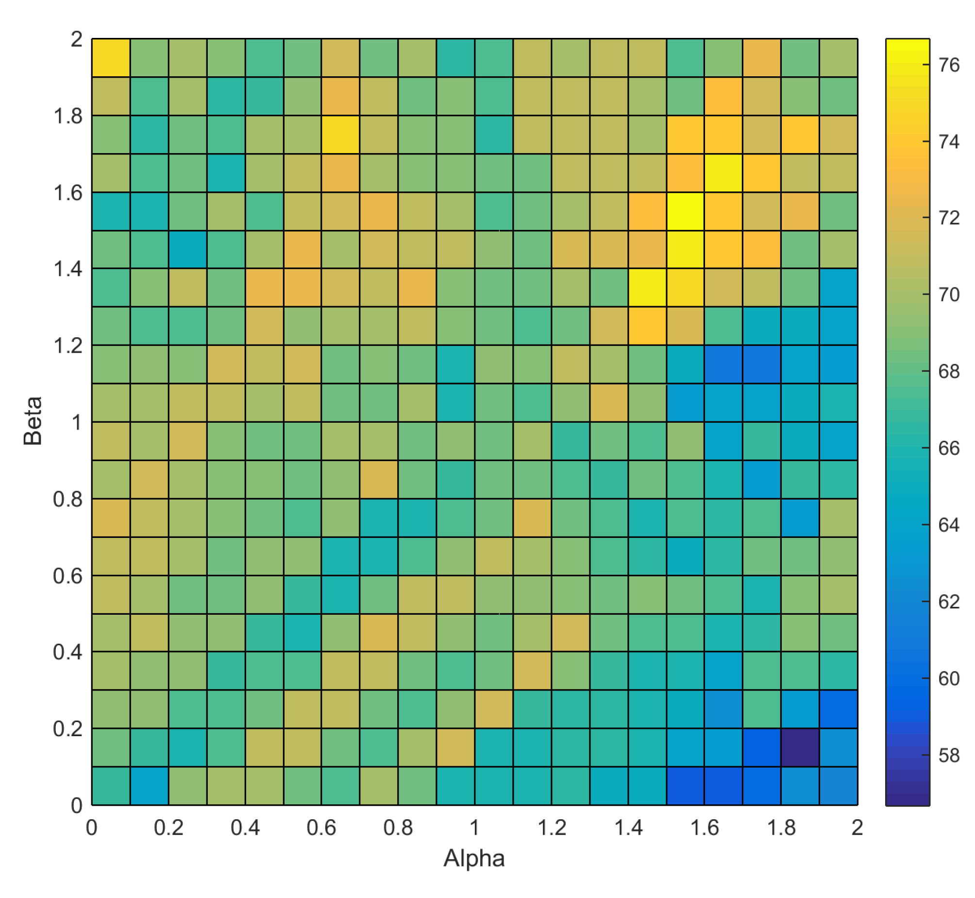
10.4. Selection of α, β and η Values

The selection of α and β is one of the crucial steps for the proposed algorithm. Depending on the α and β values, the AB Log-Det divergence can be derived into different divergence techniques [6]. The proposed algorithm performed better when $\alpha =\beta$, situation where the AB Log-Det divergence is symmetric or invariant under the permutation of its arguments. In this experiment, we have observed the performance for various values of $\alpha =\beta$ and η, and a suitable configuration of parameters for each dataset was selected.

11. Results and Discussion

The performance of the proposed Sub-ABLD algorithm is compared with the performance of the existing algorithms: CSP, JADE, MAPCSP and divCSP-WS for both the synthetic and the real BCI competition datasets. JADE algorithm performs a joint approximate diagonalization of the trial covariance matrices of the classes [45]. MAPCSP is a Bayesian algorithm that tries to find the maximum a posteriori estimates of the patterns and sources in a generative model with additive Gaussian isotropic noise [14]. The subspace implementation of divCSP-WS finds a balance between the maximization of Beta divergence between the conditional covariances of the filtered outputs for each class and the minimization of the variability within each class [1]. This algorithm contains two hyperparameters, the regularization factor λ and the real scalar ${\beta }^{\prime }$ that specifies the chosen Beta divergence. The factor λ admits an equivalence in terms of the reguralization parameter η in Sub-ABLD which link them through the mapping $\lambda \equiv \eta /(1+\eta )$, while the parameter of the Beta divergence ${\beta }_{*}^{\prime }$ was chosen in the simulations to maximize the performance .

In order to carry out a fair performance comparison, a total of six features (i.e., $p=6$) have been selected for all the algorithms. The implementation of the JADE and divCSP-WS algorithms were taken from the webpages of the authors. The baseline divCSP-WS algorithm has been downloaded from [60], while the implementation of JADE algorithm can be found at [61]. The performance comparison between all the algorithms is presented in the following subsections.

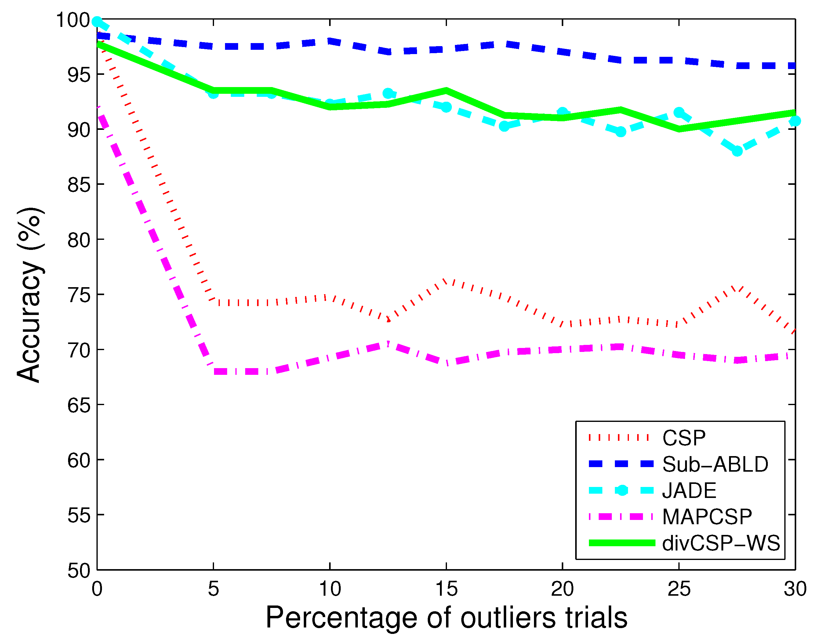
11.1. Observations for Simulated Data

To study the performance of the proposed algorithm in the presence of outliers, the experiment was done by increasing the percentage of outlier trials in the training set for both the classes. The performance of the proposed Sub-ABLD algorithm for $(\alpha ,\beta )=(1.5,1.5)$ and $\eta =1$ was obtained. The performances of the above algorithms with the increasing percentage of outliers in the training set are presented in Figure 5. It can be observed that CSP and MAPCSP perform worse in the presence of the outliers. The performances of JADE and divCSP-WS are much more robust than those of CSP and MAPCSP, but in overall the proposed Sub-ABLD algorithm seems to outperform the compared algorithms in the presence of the outliers.

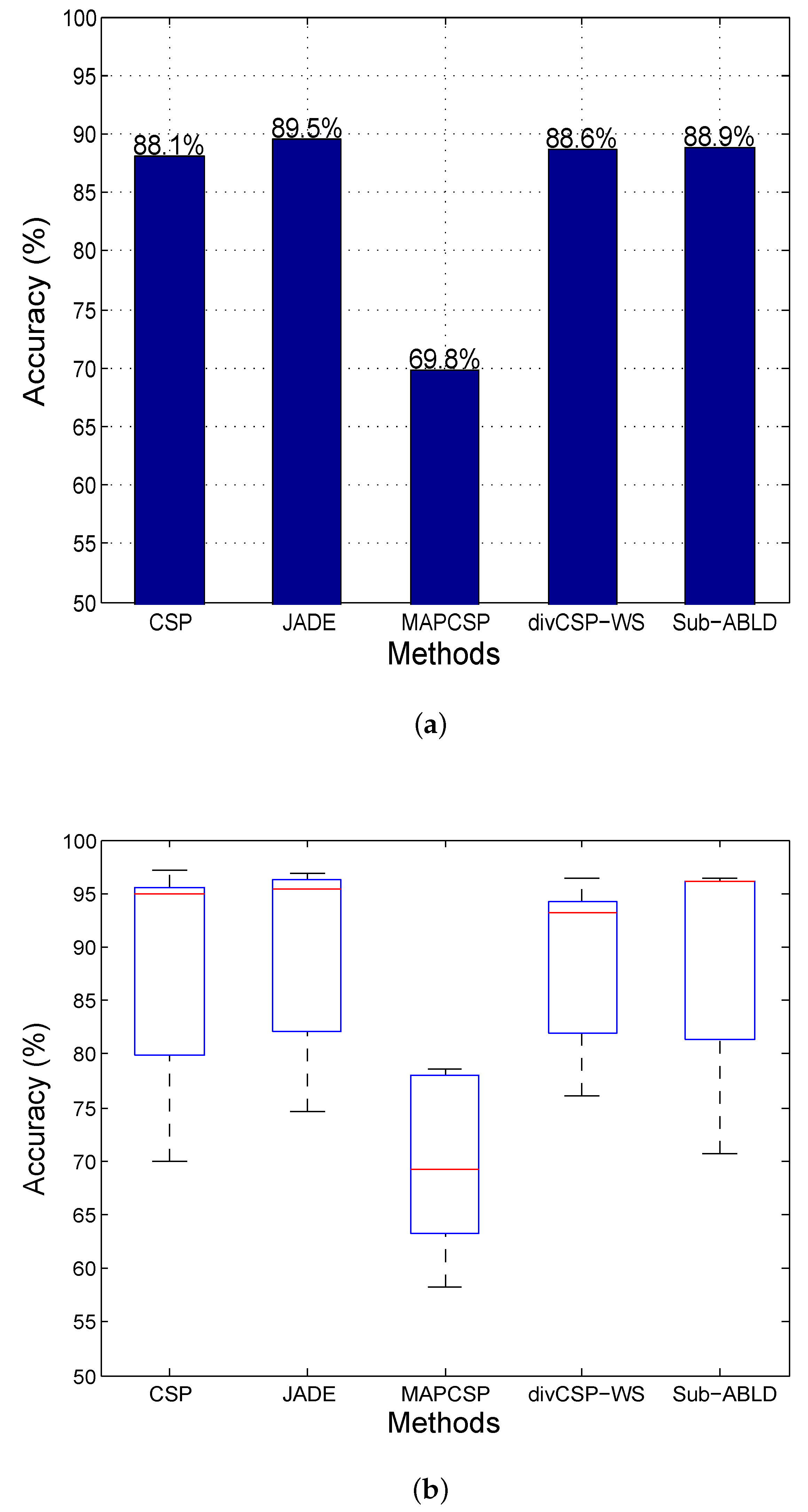
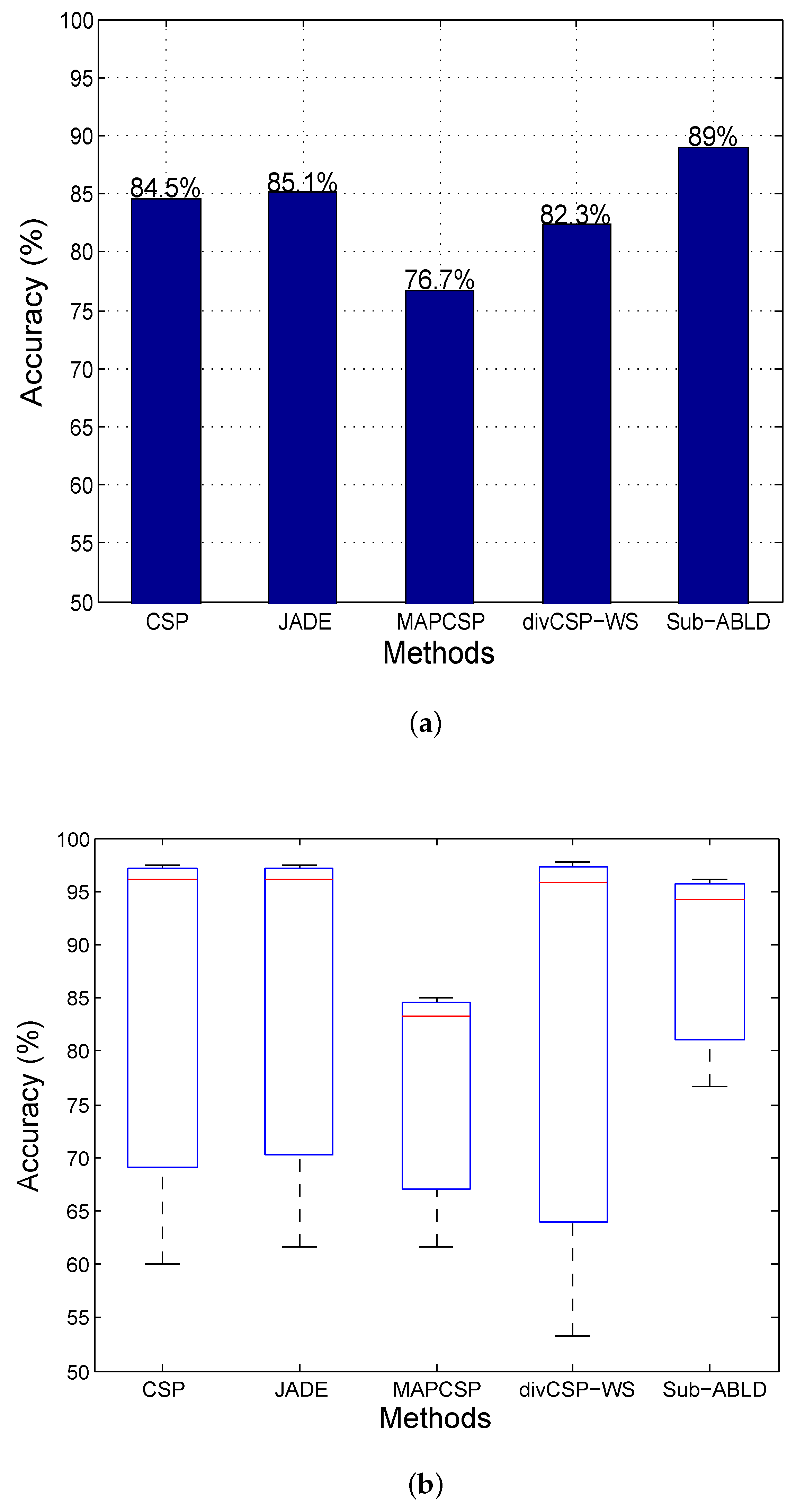
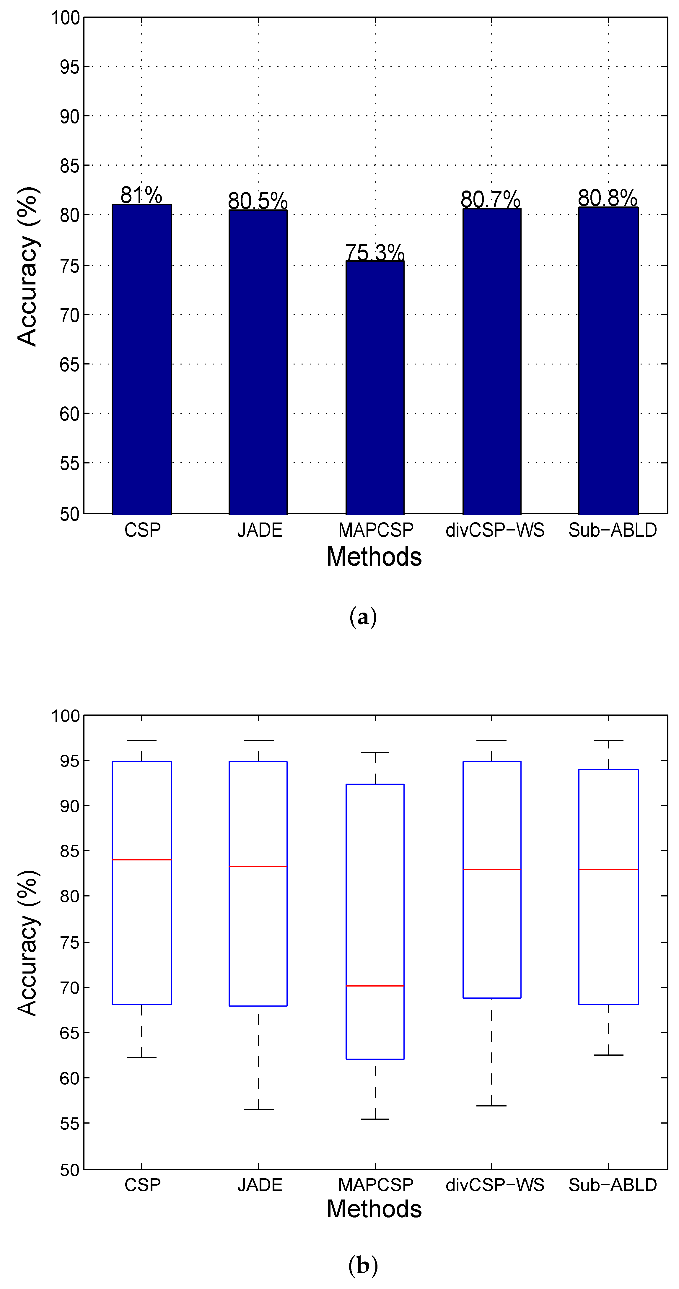
11.2. Observations for BCI Competition Datasets

In this section, the proposed algorithm is tested using three BCI competition datasets. For each dataset, the performances of the proposed algorithm for the different values of $(\alpha ,\beta )$ and η were observed. From the observation, the maximum performance of the Sub-ABLD algorithm for the particular $(\alpha ,\beta )$ and η values was selected. The selected performance is compared with the performances of other existing algorithms. Further analysis is done by using a box plot comparison for all the algorithms. The box plot analysis shows the distribution of the performances. In a box plot representation, the line inside the box represents the median performance. The upper and lower hinge of the box denote the 75-th and 25-th percentile of the overall performance distributions. The whiskers are symbolized by the two lines outside the box. The upper and lower whisker represent the maximum and minimum performance observed.

For BCI competition III dataset 3a, the Figure 6a shows the comparison of the highest average performance of the Sub-ABLD algorithm with the average performances of other existing algorithms. From the figure, it is observed that the Sub-ABLD algorithm outperforms the other existing algorithms with an average performance accuracy of $89\%$ for this dataset. The box plot comparison is shown in Figure 6b. Although, the median performance is slightly higher for CSP, JADE and divCSP, their the 25th percentile performance is much smaller than the one of the Sub-ABLD algorithm. As we will see later, is a consequence that with the Sub-ABLD algorithm the most difficult subjects have attained a significant improvement in their classification performance.

Figure 7 shows the observed average performances using BCI competition III dataset 4a. For this dataset, the algorithms JADE, Sub-ABLD and divCSP-WS perform essentially similar and slightly above than the average performance of CSP, which is 88.1%. From the box plot of the results we can observe that the 25-th percentiles for these four algorithms are also quite close.

Similar results have been obtained for the BCI competition IV dataset 2a, which are shown in Figure 8. Again the algorithms JADE, Sub-ABLD and divCSP-WS perform essentially the same as CSP, which average performance is 81%. In the box plot we can observe that the quartiles of these algorithms are approximately coincident.

To analyze the effect of performance for different divergences, we varied the parameters $(\alpha ,\beta )$ for a single subject (Subject k6 from BCI competition III dataset 3a, which is one of the subjects with worst performance for the experiment) and obtained the corresponding performance. The values of $(\alpha ,\beta )$ are varied to cover the interval $[0,2]\times [0,2]$ with a mesh of 0.1 spacings. The observed performance is shown in Figure 9. This figure reveals a tendency to improve the classification accuracy of the worst user for values of α and β that are close to the diagonal and large enough so they can effectively down-weight the contribution in the estimating equations coming from the largest and smallest generalized eigenvalues.

The proposed Sub-ABLD algorithm has been tested on both simulated and real EEG signals. On one hand, the results with synthetic data indicate that the proposed Sub-ABLD exhibits a certain robustness to the presence of outliers trials in the dataset. On the other hand, the analysis of real EEG signals is also challenging because of the possible presence of artifacts and non-stationarities. We have presented the performance of the Sub-ABLD algorithm using several real BCI datasets. For BCI competition III dataset 3a, we can observe that the proposed Sub-ABLD algorithm also outperforms the other algorithms. Whereas, the performance of the proposed algorithm is almost similar to the one obtained by JADE, divCSP-WS and CSP in the other two datasets, i.e., for the BCI competition III dataset 4a and BCI competition IV dataset 2a. Additionally, the analysis of the box-plots reveals that the proposed Sub-ABLD algorithm increased the classification performance of the subjects that do not perform well for the other methods. At the same time, it retained an almost similar performance for the remaining subjects. These observations meet our initial goal of developing a robust algorithm. The classification performance is also affected by the regularization parameter η that controls the penalty term. In general, the data with outliers give the best performance for the higher values of η and, otherwise, smaller values are preferable. In this study, the value of η has been kept constant across subjects in each dataset.

12. Conclusions

In this paper, we have explained how one can be able to use and optimize the recently proposed family of Alpha-Beta Log-Det divergences. For this purpose, we have summarized the key properties of these divergences and derived an original explicit formula for their gradient. In this work, we have adopted as an illustrative example of application the problem of spatial filter selection for the classification of two class imagery movements. We have reexamined the relation between the Common Spatial Pattern criterion with a predefined number of spatial filters for each class and its interpretation as an Alpha-Beta Log-Det divergence optimization problem, to show that a scaling factor in one of the arguments of the divergence is necessary for the equivalence of the solutions. We have proposed a subspace algorithm (Sub-ABLD) for obtaining the spatial filters that retain the discriminative information of two class MI movements. This algorithm was tested with synthetic and real datasets and compared with the other existing algorithms. The simulations have confirmed the possibility to tune up the hyperparameters of the divergence so as to improve the robustness of the obtained solutions without deteriorating the expected accuracy.

References

1. Samek, W.; Kawanabe, M.; Müller, K.R. Divergence-based framework for common spatial patterns algorithms. IEEE Rev. Biomed. Eng. 2014, 7, 50–72. [Google Scholar] [CrossRef] [PubMed]
2. Huang, Z.; Wang, R.; Shan, S.; Li, X.; Chen, X. Log-Euclidean Metric Learning on Symmetric Positive Definite Manifold with Application to Image Set Classification. In Proceedings of the 32nd International Conference on Machine Learning (ICML), Lille, France, 6–11 July 2015.
3. Salzmann, M.; Hartley, R. Dimensionality Reduction on SPD Manifolds: The Emergence of Geometry-Aware Methods. IEEE Trans. Pattern Anal. Mach. Intell. 2016. [Google Scholar] [CrossRef]
4. Sra, S.; Hosseini, R. Geometric Optimization in Machine Learning Algorithmic Advances in Riemannian Geometry and Applications: For Machine Learning, Computer Vision, Statistics, and Optimization; Springer: Berlin/Heidelberg, Germany, 2016. [Google Scholar]
5. Horev, I.; Yger, F.; Sugiyama, M. Geometry-aware principal component analysis for symmetric positive definite matrices. In Proceedings of the 7th Asian Conference on Machine Learning, Hong Kong, China, 20–22 November 2015; pp. 1–16.
6. Cichocki, A.; Cruces, S.; Amari, S.i. Log-Determinant Divergences Revisited: Alpha-Beta and Gamma Log-Det Divergences. Entropy 2015, 17, 2988–3034. [Google Scholar] [CrossRef]
7. Minh, H.Q. Infinite-dimensional Log-Determinant divergences II: Alpha-Beta divergences. arXiv 2017. [Google Scholar]
8. Dornhege, G. Toward Brain-Computer Interfacing; MIT Press: Cambridge, MA, USA, 2007. [Google Scholar]
9. Wolpaw, J.; Wolpaw, E.W. Brain-computer Interfaces: Principles and Practice; Oxford University Press: Oxford, UK, 2012. [Google Scholar]
10. Pfurtscheller, G.; Da Silva, F.L. Event-related EEG/MEG synchronization and desynchronization: Basic principles. Clin. Neurophysiol. 1999, 110, 1842–1857. [Google Scholar] [CrossRef]
11. Fukunaga, K.; Koontz, W.L.G. Application of the Karhunen-Loeve Expansion to Feature Selection and Ordering. IEEE Trans. Comput. 1970, C-19, 440–447. [Google Scholar] [CrossRef]
12. Koles, Z.J. The quantitative extraction and topographic mapping of the abnormal components in the clinical EEG. Electroencephalogr. Clin. Neurophysiol. 1991, 79, 440–447. [Google Scholar] [CrossRef]
13. Ramoser, H.; Müller-Gerking, J.; Pfurtscheller, G. Optimal spatial filtering of single trial EEG during imagined hand movement. IEEE Trans. Rehabil. Eng. 2000, 8, 441–446. [Google Scholar] [CrossRef] [PubMed]
14. Wu, W.; Chen, Z.; Gao, X.; Li, Y.; Brown, E.N.; Gao, S. Probabilistic common spatial patterns for multichannel EEG analysis. IEEE Trans. Pattern Anal. Mach. Intell. 2015, 37, 639–653. [Google Scholar] [CrossRef] [PubMed]
15. Bhatia, R. Matrix Analysis; Graduate Texts in Mathematics; Springer: Berlin/Heidelberg, Germany, 1997. [Google Scholar]
16. Wang, H. Harmonic mean of Kullback–Leibler divergences for optimizing multi-class EEG spatio-temporal filters. Neural Process. Lett. 2012, 36, 161–171. [Google Scholar] [CrossRef]
17. Samek, W.; Blythe, D.; Müller, K.R.; Kawanabe, M. Robust spatial filtering with beta divergence. In Proceedings of the Advances in Neural Information Processing Systems, Stateline, NV, USA, 5–10 December 2013; pp. 1007–1015.
18. Cichocki, A.; Amari, S. Families of Alpha- Beta- and Gamma- Divergences: Flexible and Robust Measures of Similarities. Entropy 2010, 12, 1532–1568. [Google Scholar] [CrossRef]
19. Brandl, S.; Müller, K.R.; Samek, W. Robust common spatial patterns based on Bhattacharyya distance and Gamma divergence. In Proceedings of the 2015 3rd International Winter Conference on Brain-Computer Interface (BCI), Jeongsun-Kun, Korea, 12–14 January 2015; pp. 1–4.
20. Tao, T. Topics in Random Matrix Theory; American Mathematical Society: Providence, RI, USA, 2012; Volume 132. [Google Scholar]
21. Blankertz, B.; Kawanabe, M.; Tomioka, R.; Hohlefeld, F.; Müller, K.R.; Nikulin, V.V. Invariant common spatial patterns: Alleviating nonstationarities in brain-computer interfacing. In Proceedings of the Advances in Neural Information Processing Systems, Vancouver, BC, Canada, 3–6 December 2007; pp. 113–120.
22. Lotte, F.; Guan, C. Spatially regularized common spatial patterns for EEG classification. In Proceedings of the 2010 20th International Conference on Pattern Recognition (ICPR), Istanbul, Turkey, 23–26 August 2010; pp. 3712–3715.
23. Kang, H.; Nam, Y.; Choi, S. Composite common spatial pattern for subject-to-subject transfer. IEEE Signal Process. Lett. 2009, 16, 683–686. [Google Scholar] [CrossRef]
24. Lotte, F.; Guan, C. Learning from other subjects helps reducing brain-computer interface calibration time. In Proceedings of the 2010 IEEE International Conference on Acoustics Speech and Signal Processing (ICASSP), Dallas, TX, USA, 14–19 March 2010; pp. 614–617.
25. Lu, H.; Plataniotis, K.N.; Venetsanopoulos, A.N. Regularized common spatial patterns with generic learning for EEG signal classification. In Proceedings of the 2009 Annual International Conference of the IEEE Engineering in Medicine and Biology Society, Minneapolis, MN, USA, 3–6 September 2009; pp. 6599–6602.
26. Xinyi Yong, R.K.W.; Birch, G.E. Robust Common Spatial Patterns for EEG Signal Preprocessing. In Proceedings of the IEEE EMBS 30th Annual International Conference, Vancouver, BC, Canada, 20–25 August 2008; pp. 2087–2090.
27. Kawanabe, M.; Vidaurre, C. Improving BCI performance by modified common spatial patterns with robustly averaged covariance matrices. In Proceedings of the World Congress on Medical Physics and Biomedical Engineering, Munich, Germany, 7–12 September 2009.
28. Samek, W.; Binder, A.; Müller, K.R. Multiple kernel learning for brain-computer interfacing. In Proceedings of the 2013 35th Annual International Conference of the IEEE Engineering in Medicine and Biology Society (EMBC), Osaka, Japan, 3–7 July 2013; pp. 7048–7051.
29. Lotte, F.; Guan, C. Regularizing common spatial patterns to improve BCI designs: unified theory and new algorithms. IEEE Trans. Biomed. Eng. 2011, 58, 355–362. [Google Scholar] [CrossRef] [PubMed]
30. Arvaneh, M.; Guan, C.; Ang, K.K.; Quek, H.C. Spatially sparsed common spatial pattern to improve BCI performance. In Proceedings of the 2011 IEEE International Conference on Acoustics, Speech and Signal Processing (ICASSP), Prague, Czech Republic, 22–27 May 2011; pp. 2412–2415.
31. Farquhar, J.; Hill, N.; Lal, T.N.; Schölkopf, B. Regularised CSP for sensor selection in BCI. In Proceedings of the 3rd International BCI workshop, Graz, Austria, 21–24 September 2006; pp. 1–2.
32. Yong, X.; Ward, R.K.; Birch, G.E. Sparse spatial filter optimization for EEG channel reduction in brain-computer interface. In Proceedings of the IEEE International Conference on Acoustics, Speech and Signal Processing (ICASSP 2008), Las Vegas, NV, USA, 31 March–4 April 2008; pp. 417–420.
33. Kawanabe, M.; Vidaurre, C.; Scholler, S.; Müller, K.R. Robust common spatial filters with a maxmin approach. In Proceedings of the 2009 Annual International Conference of the IEEE Engineering in Medicine and Biology Society, Minneapolis, MN, USA, 3–6 September 2009; pp. 2470–2473.
34. Kawanabe, M.; Samek, W.; Müller, K.R.; Vidaurre, C. Robust common spatial filters with a maxmin approach. Neural Comput. 2014, 26, 349–376. [Google Scholar] [CrossRef] [PubMed]
35. Wang, H.; Tang, Q.; Zheng, W. L1-norm-based common spatial patterns. IEEE Trans. Biomed. Eng. 2012, 59, 653–662. [Google Scholar] [CrossRef] [PubMed]
36. Park, J.; Chung, W. Common spatial patterns based on generalized norms. In Proceedings of the 2013 International Winter Workshop on Brain-Computer Interface (BCI), Jeongsun-kun, Korea, 18–20 February 2013; pp. 39–42.
37. Von Bünau, P.; Meinecke, F.C.; Király, F.C.; Müller, K.R. Finding stationary subspaces in multivariate time series. Phys. Rev. Lett. 2009, 103, 214101. [Google Scholar] [CrossRef] [PubMed]
38. Samek, W.; Kawanabe, M.; Vidaurre, C. Group-wise stationary subspace analysis–A novel method for studying non-stationarities. In Proceedings of the International Brain–Computer Interfacing Conference, Graz, Austria, 22–24 September 2011; pp. 16–20.
39. Samek, W.; Müller, K.R.; Kawanabe, M.; Vidaurre, C. Brain-computer interfacing in discriminative and stationary subspaces. In Proceedings of the 2012 Annual International Conference of the IEEE Engineering in Medicine and Biology Society (EMBC), San Diego, CA, USA, 28 August–1 September 2012; pp. 2873–2876.
40. Von Bünau, P.; Meinecke, F.C.; Scholler, S.; Müller, K.R. Finding stationary brain sources in EEG data. In Proceedings of the 2010 Annual International Conference of the IEEE Engineering in Medicine and Biology Society (EMBC), Buenos Aires, Argentina, 31 August–4 September 2010; pp. 2810–2813.
41. Arvaneh, M.; Guan, C.; Ang, K.K.; Quek, C. Optimizing spatial filters by minimizing within-class dissimilarities in electroencephalogram-based brain–computer interface. IEEE Trans. Neural Netw. Learn. Syst. 2013, 24, 610–619. [Google Scholar] [CrossRef] [PubMed]
42. Müller-Gerking, J.; Pfurtscheller, G.; Flyvbjerg, H. Designing optimal spatial filters for single-trial EEG classification in a movement task. Clin. Neurophysiol. 1999, 110, 787–798. [Google Scholar] [CrossRef]
43. Allwein, E.L.; Schapire, R.E.; Singer, Y. Reducing multiclass to binary: A unifying approach for margin classifiers. J. Mach. Learn. Res. 2001, 1, 113–141. [Google Scholar]
44. Dornhege, G.; Blankertz, B.; Curio, G.; Müller, K.R. Boosting bit rates in noninvasive EEG single-trial classifications by feature combination and multiclass paradigms. IEEE Trans. Biomed. Eng. 2004, 51, 993–1002. [Google Scholar] [CrossRef] [PubMed]
45. Grosse-Wentrup, M.; Buss, M. Multiclass common spatial patterns and information theoretic feature extraction. IEEE Trans. Biomed. Eng. 2008, 55, 1991–2000. [Google Scholar] [CrossRef] [PubMed]
46. Naeem, M.; Brunner, C.; Leeb, R.; Graimann, B.; Pfurtscheller, G. Separability of four-class motor imagery data using independent components analysis. J. Neural Eng. 2006, 3, 208–216. [Google Scholar] [CrossRef] [PubMed]
47. Barachant, A.; Bonnet, S.; Congedo, M.; Jutten, C. Multiclass brain–Computer interface classification by Riemannian geometry. IEEE Trans. Biomed. Eng. 2012, 59, 920–928. [Google Scholar] [CrossRef] [PubMed] [Green Version]
48. Zhang, H.; Yang, H.; Guan, C. Bayesian learning for spatial filtering in an EEG-based brain–computer interface. IEEE Trans. Neural Netw. Learn. Syst. 2013, 24, 1049–1060. [Google Scholar] [CrossRef] [PubMed]
49. Barber, D. Bayesian Reasoning and Machine Learning; Cambridge University Press: Cambridge, UK, 2012. [Google Scholar]
50. Edelman, A.; Arias, T.A.; Smith, S.T. The geometry of algorithms with orthogonality constraints. SIAM J. Matrix Anal. Appl. 1998, 20, 303–353. [Google Scholar] [CrossRef]
51. Amari, S.I. Natural gradient works efficiently in learning. Neural Comput. 1998, 10, 251–276. [Google Scholar] [CrossRef]
52. Cruces, S.; Cichocki, A.; Amari, S. From Blind Signal Extraction to Blind Instantaneous Signal Separation. IEEE Trans. Neural Netw. 2004, 15, 859–873. [Google Scholar] [CrossRef] [PubMed]
53. Nishimori, Y. Learning algorithm for ICA by geodesic flows on orthogonal group. In Proceedings of the International Joint Conference on Neural Networks (IJCNN), Washington, DC, USA, 10–16 July 1999; pp. 933–938.
54. BCI Competition III. Available online: http://www.bbci.de/competition/iii/ (accessed on 26 August 2014).
55. BCI Competition IV. Available online: http://www.bbci.de/competition/iv/ (accessed on 26 August 2014).
56. Schlögl, A.; Lee, F.; Bischof, H.; Pfurtscheller, G. Characterization of four-class motor imagery EEG data for the BCI-competition 2005. J. Neural Eng. 2005, 2, L14. [Google Scholar] [CrossRef] [PubMed]
57. Blankertz, B.; Müller, K.R.; Krusienski, D.J.; Schalk, G.; Wolpaw, J.R.; Schlögl, A.; Pfurtscheller, G.; Millan, J.R.; Schröder, M.; Birbaumer, N. The BCI competition III: Validating alternative approaches to actual BCI problems. IEEE Trans. Neural Syst. Rehabil. Eng. 2006, 14, 153–159. [Google Scholar] [CrossRef] [PubMed]
58. Tangermann, M.; Müller, K.R.; Aertsen, A.; Birbaumer, N.; Braun, C.; Brunner, C.; Leeb, R.; Mehring, C.; Miller, K.J.; Mueller-Putz, G.; et al. Review of the BCI competition IV. Front. Neurosci. 2012, 6, 55. [Google Scholar]
59. Duda, R.O.; Hart, P.E. Pattern Classification and Scene Analysis; Wiley: New York, NY, USA, 1973; Volume 3. [Google Scholar]
60. The Divergence Methods Web Site. Available online: http://www.divergence-methods.org (accessed on 4 April 2016).
61. Machine Learning in Neural Engineering. Available online: http://brain-computer-interfaces.net/ (accessed on 29 January 2015).
62. Li, R. Rayleigh Quotient Based Optimization Methods For Eigenvalue Problems. In Summary of Lectures Delivered at Gene Golub SIAM Summer School 2013; Fudan University: Shanghai, China, 2013; pp. 1–27. [Google Scholar]
Figure 1. This illustration shows the AB log-det divergence D A B ( α , β ) ( P Q ) positioned in a plane as a function of their real pair of hyperparameters ( α , β ) . It is clear from the figure, that the parameterization smoothly connects several relevant positive definite matrix divergences, like: the squared Riemannian metric ( α = 0 , β = 0 ), the KL matrix divergence or Stein’s loss ( α = 1 , β = 0 ), the dual KL matrix divergence ( α = 0 , β = 1 ), and the S-divergence ( α = 1 2 , β = 1 2 ) among others.
Entropy 19 00089 g001
Figure 2. Illustration of the strictly monotonous ascending transformation g ( · ) that, through Equation (56), maps eigenvalues of the matrix pencil ( p ( c 1 ) P , C o v ( x ) ) into the eigenvalues of the matrix pencil ( P , Q ) , in a case where the sample probabilities of the classes are uniform p ( c 1 ) = p ( c 2 ) . Note that the eigenvalues of the first pencil are bounded in the interval ( 0 , 1 ) , while the domain of the eigenvalues of the second pencil is ( 0 , ) .
Entropy 19 00089 g002
Figure 3. Illustration of the behavior of the AB log-det divergence D A B ( α , β ) ( μ , 1 ) , and of its associated weight function w α , β ( μ ) , versus μ for different values of α = β . Note that μ is shown in log-scale. (a) Squared Riemannian metric for α = β = 0 (upper plot) and its weight function (lower plot); (b) Power Log-det divergence for α = β = 1 (upper plot) and its weight function (lower plot).
Entropy 19 00089 g003
Figure 4. Illustration of the behavior of the AB log-det divergence D A B ( α , β ) ( μ , 1 ) , and of its associated weight function w α , β ( μ ) , versus μ for different values of α β . Note that μ is shown in log-scale. (a) Kullback–Leibler (KL) positive definite matrix divergence for α = 1 , β = 0 , and its weight function (lower plot); (b) Dual KL positive definite matrix div. for α = 0 , β = 1 , and its weight function (lower plot).
Entropy 19 00089 g004
Figure 5. Performance comparison of the proposed algorithm Sub-ABLD ( η = 1 , α = β = 1.5 ) with CSP, JADE, MAPCSP and divCSP-WS ( λ = 0.5 , β * = 0.25 ), versus the percentage of outlier trials.
Entropy 19 00089 g005
Figure 6. (a) Performance comparison of the proposed algorithm Sub-ABLD ( η = 2 , α = β = 1.5 ) with CSP, JADE, MAPCSP and divCSP-WS ( λ = 0.66 , β * = 1 ) using BCI competition III dataset 3a and (b) its corresponding boxplot.
Entropy 19 00089 g006
Figure 7. (a) Performance comparison of the proposed algorithm Sub-ABLD ( η = 0.5 , α = β = 2 ) with CSP, JADE, MAPCSP and divCSP-WS ( λ = 0.33 , β * = 0.5 ) using BCI competition datasets III dataset 4a and (b) its corresponding boxplot.
Entropy 19 00089 g007
Figure 8. (a) Performance comparison of the proposed algorithm Sub-ABLD ( η = 0.25 , α = β = 1.25 ) with CSP, JADE, MAPCSP and divCSP-WS ( λ = 0.2 , β * = 0 ) using BCI competition datasets IV dataset 2a and (b) its corresponding boxplot.
Entropy 19 00089 g008
Figure 9. Results of the Sub-ABLD algorithm for the subject k6 from BCI competition III dataset 3a. This figure illustrates the changes in the average classification performance with respect to the variation of the parameters α and β. Relatively good performance results are obtained close to the diagonal and for moderately large values of the parameters.
Entropy 19 00089 g009