
Use of Accumulated Entropies for Automated Detection of Congestive Heart Failure in Flexible Analytic Wavelet Transform Framework Based on Short-Term HRV Signals


Abstract
:1. Introduction
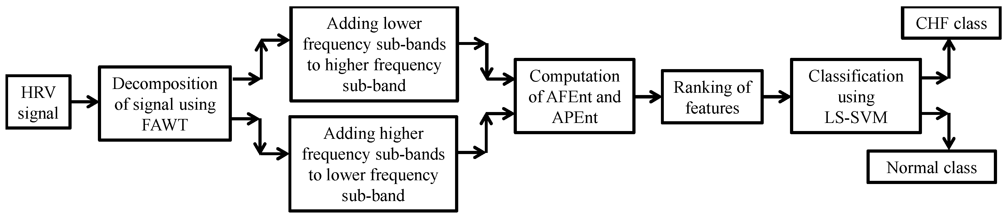
2. Methodology
2.1. HRV Dataset
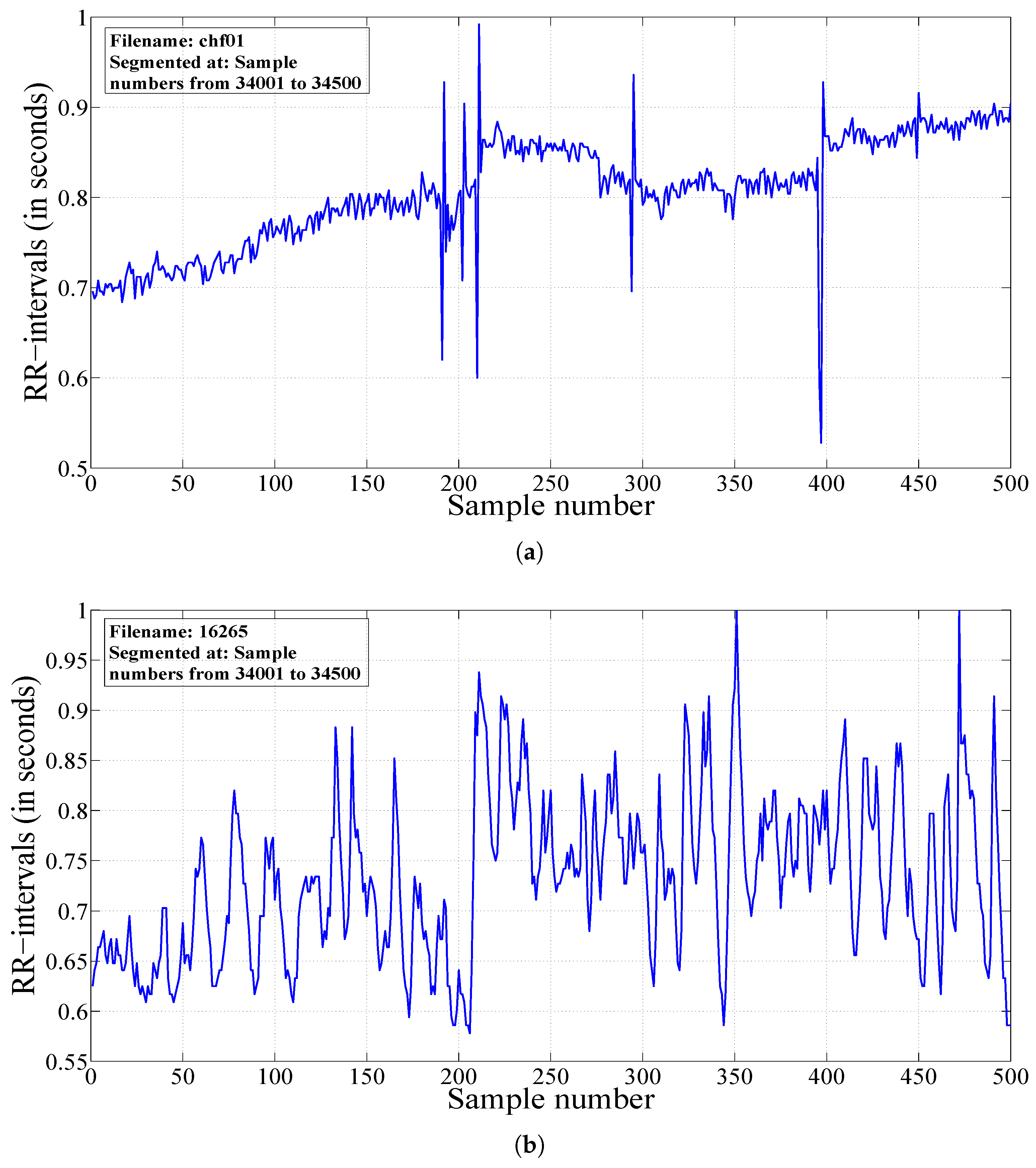
2.2. Segmentation of HRV Signals
2.3. Features Studied in This Work
2.3.1. Permutation Entropy
2.3.2. Fuzzy Entropy
- First, the sequences of length e are extracted from the HRV signal.
- Computation of the similarity degree between two sequences (j-th and k-th) using the fuzzy function [39] as follows:where μ, f and g represent the fuzzy function, the gradient and the width of the fuzzy similarity boundary, respectively and is the maximum absolute difference of the two sequence lengths.
- Computation of as follows [39]:where P denotes the total number of samples present in the HRV signal.
- Finally, the FEnt can be computed as follows [39]:
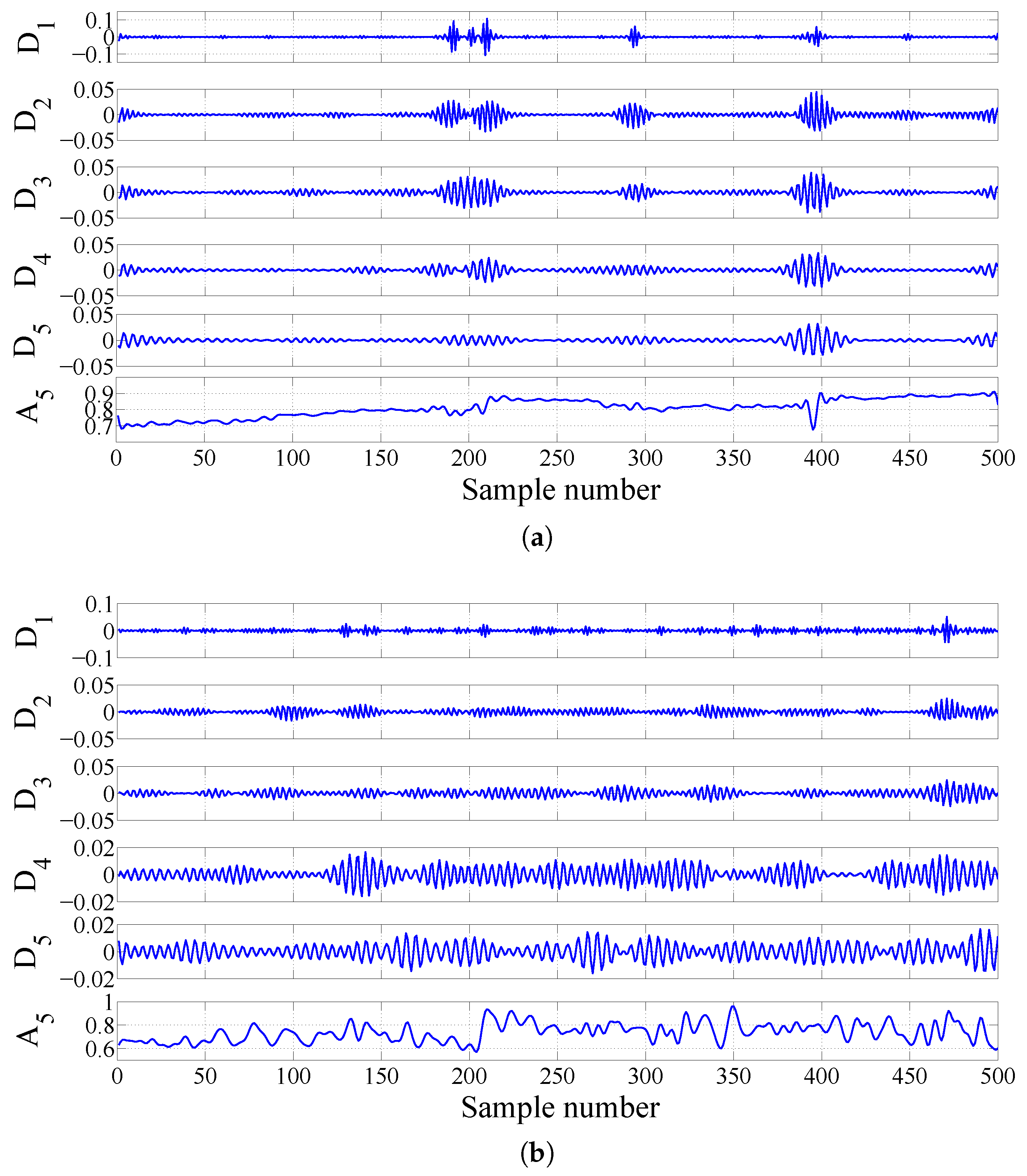
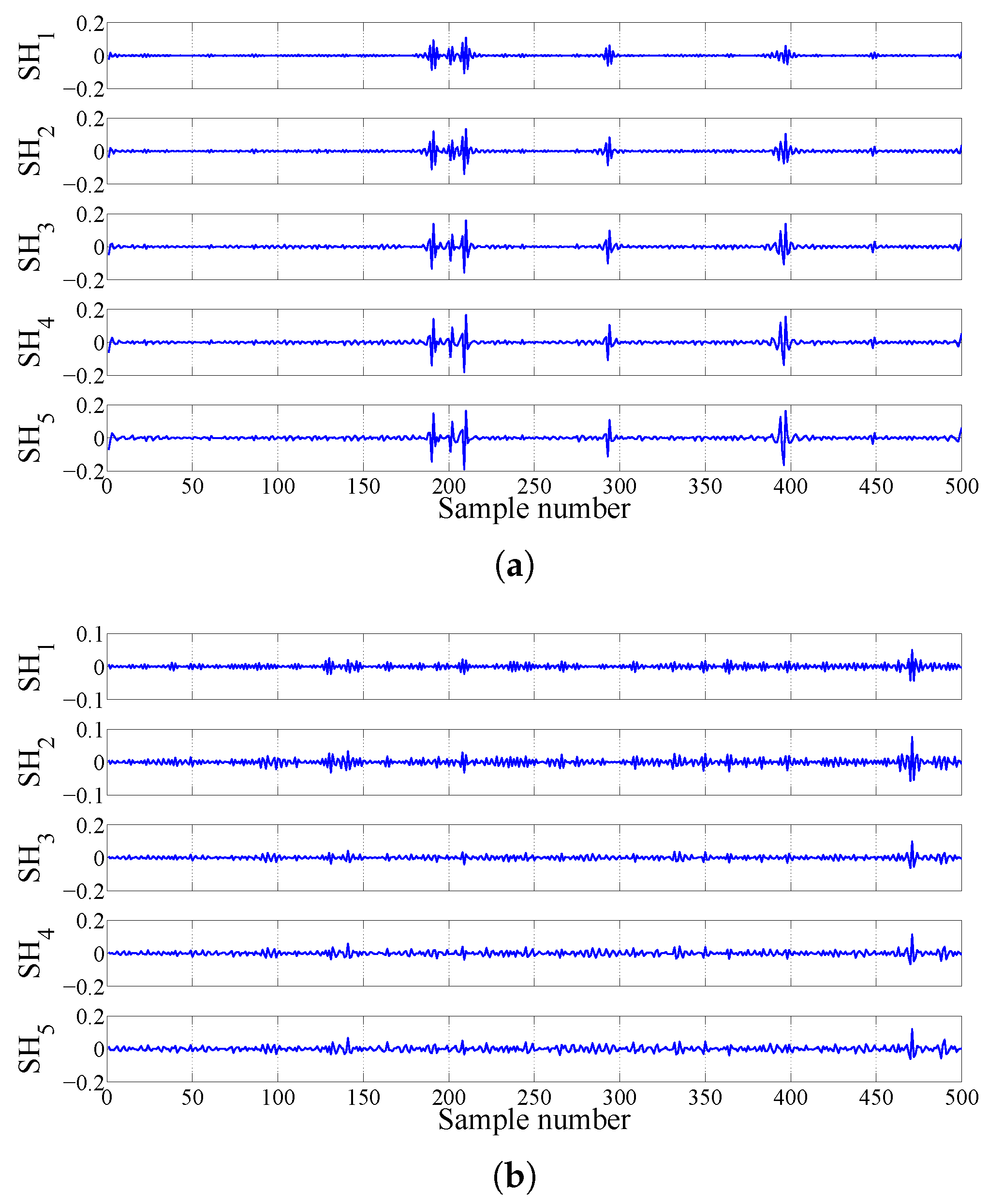
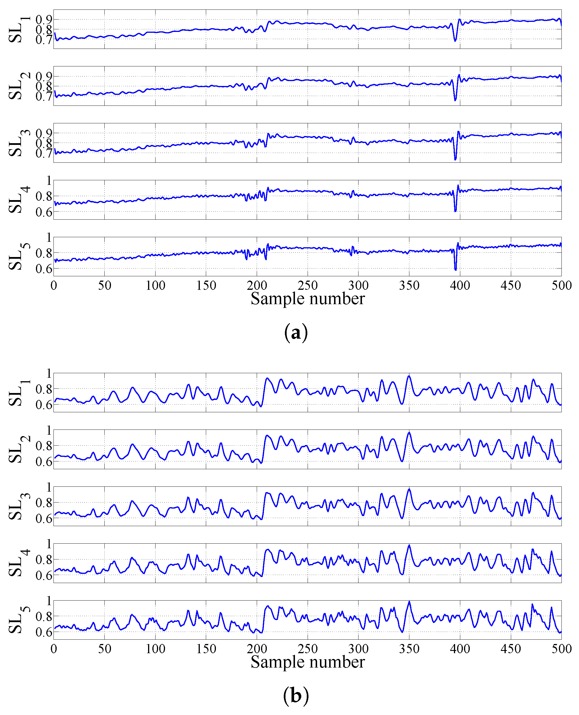
2.3.3. FAWT-Based Accumulated Entropies
2.4. Ranking and Classification
3. Results
3.1. Results with a Signal Length of 500 Samples
3.1.1. Results for Unbalanced Dataset 1
3.1.2. Results for Unbalanced Dataset 2
3.1.3. Results for Balanced Dataset 1
3.1.4. Results for Balanced Dataset 2
3.2. Results with a Signal Length of 1000 Samples
3.3. Results with a 2000-Sample Signal Length
4. Discussion
5. Conclusions
Author Contributions
Conflicts of Interest
References
- Ponikowski, P.; Anker, S.D.; AlHabib, K.F.; Cowie, M.R.; Force, T.L.; Hu, S.; Jaarsma, T.; Krum, H.; Rastogi, V.; Rohde, L.E.; et al. Heart failure: preventing disease and death worldwide. ESC Heart Fail. 2014, 1, 4–25. [Google Scholar] [CrossRef]
- National Heart, Lung and Blood Institute, What Is Heart Failure? 2015. Available online: https://www.nhlbi.nih.gov/health/health-topics/topics/hf/ (accessed on 15 January 2017).
- Pazos-López, P.; Peteiro-Vázquez, J.; Carcía-Campos, A.; García-Bueno, L.; de Torres, J.P.A.; Castro-Beiras, A. The causes, consequences, and treatment of left or right heart failure. Vasc. Health Risk Manag. 2011, 7, 237–254. [Google Scholar] [PubMed]
- Jong, T.L.; Chang, B.; Kuo, C.D. Optimal timing in screening patients with congestive heart failure and healthy subjects during circadian observation. Ann. Biomed. Eng. 2011, 39, 835–849. [Google Scholar] [CrossRef] [PubMed]
- Khaled, A.S.; Owis, M.I.; Mohamed, A.S.A. Employing time-domain methods and Poincaré plot of heart rate variability signals to detect congestive heart failure. BIME J. 2006, 6, 35–41. [Google Scholar]
- Acharya, U.R.; Kannathal, N.; Krishnan, S.M. Comprehensive analysis of cardiac health using heart rate signals. Physiol. Meas. 2004, 25, 1139–1151. [Google Scholar]
- Sood, S.; Kumar, M.; Pachori, R.B.; Acharya, U.R. Application of empirical mode decomposition-based features for analysis of normal and CAD heart rate signals. J. Mech. Med. Biol. 2016, 16, 1640002. [Google Scholar] [CrossRef]
- Giri, D.; Acharya, U.R.; Martis, R.J.; Sree, S.V.; Lim, T.C.; Vi, T.A.; Suri, J.S. Automated diagnosis of coronary artery disease affected patients using LDA, PCA, ICA and discrete wavelet transform. Knowl. Based Syst. 2013, 37, 274–282. [Google Scholar] [CrossRef]
- Patidar, S.; Pachori, R.B.; Acharya, U.R. Automated diagnosis of coronary artery disease using tunable-Q wavelet transform applied on heart rate signals. Knowl. Based Syst. 2015, 82, 1–10. [Google Scholar] [CrossRef]
- Chua, K.C.; Chandran, V.; Acharya, U.R.; Lim, C.M. Cardiac state diagnosis using higher order spectra of heart rate variability. J. Med. Eng. Technol. 2008, 32, 145–155. [Google Scholar] [CrossRef] [PubMed]
- Acharya, U.R.; Sankaranarayanan, M.; Nayak, J.; Xiang, C.; Tamura, T. Automatic identification of cardiac health using modeling techniques: A comparative study. Inf. Sci. 2008, 178, 4571–4582. [Google Scholar] [CrossRef]
- Stein, P.K.; Domitrovich, P.P.; Kleiger, R.E.; Schechtman, K.B.; Rottman, J.N. Clinical and demographic determinants of heart rate variability in patients post myocardial infarction: insights from the cardiac arrhythmia suppression trial (CAST). Clin. Cardiol. 2000, 23, 187–194. [Google Scholar] [CrossRef] [PubMed]
- Mussalo, H.; Vanninen, E.; Ikäheimo, R.; Laitinen, T.; Laakso, M.; Länsimies, E.; Hartikainen, J. Heart rate variability and its determinants in patients with severe or mild essential hypertension. Clin. Physiol. 2001, 21, 594–604. [Google Scholar] [CrossRef] [PubMed]
- Malliani, A.; Lombardi, F.; Pagani, M.; Cerutti, S. Power spectral analysis of cardiovascular variability in patients at risk for sudden cardiac death. J. Cardiovasc. Electrophysiol. 1994, 5, 274–286. [Google Scholar] [CrossRef] [PubMed]
- Pachori, R.B.; Avinash, P.; Shashank, K.; Sharma, R.; Acharya, U.R. Application of empirical mode decomposition for analysis of normal and diabetic RR-interval signals. Expert Syst. Appl. 2015, 42, 4567–4581. [Google Scholar] [CrossRef]
- Acharya, U.R.; Vidya, K.S.; Ghista, D.N.; Lim, W.J.E.; Molinari, F.; Sankaranarayanan, M. Computer-aided diagnosis of diabetic subjects by heart rate variability signals using discrete wavelet transform method. Knowl. Based Syst. 2015, 81, 56–64. [Google Scholar] [CrossRef]
- Pachori, R.B.; Kumar, M.; Avinash, P.; Shashank, K.; Acharya, U.R. An improved online paradigm for screening of diabetic patients using RR-interval signals. J. Mech. Med. Biol. 2016, 16, 1640003. [Google Scholar] [CrossRef]
- Nolan, J.; Batin, P.D.; Andrews, R.; Lindsay, S.J.; Brooksby, P.; Mullen, M.; Baig, W.; Flapan, A.D.; Cowley, A.; Prescott, R.J.; et al. Prospective study of heart rate variability and mortality in chronic heart failure. Circulation 1998, 98, 1510–1516. [Google Scholar] [CrossRef] [PubMed]
- Hadase, M.; Azuma, A.; Zen, K.; Asada, S.; Kawasaki, T.; Kamitani, T.; Kawasaki, S.; Sugihara, H.; Matsubara, H. Very low frequency power of heart rate variability is a powerful predictor of clinical prognosis in patients with congestive heart failure. Circ. J. 2004, 68, 343–347. [Google Scholar] [CrossRef] [PubMed]
- Musialik-ydka, A.; Sredniawa, B.; Pasyk, S. Heart rate variability in heart failure. Kardiol. Polska 2003, 58, 10–16. [Google Scholar]
- Asyali, M.H. Discrimination Power of Long-Term Heart Rate Variability Measures. In Proceedings of the 25th Annual International Conference of the IEEE Engineering in Medicine and Biology Society, Cancun, Mexico, 17–21 September 2003; Volume 1, pp. 200–203.
- Guzzetti, S.; Mezzetti, S.; Magatelli, R.; Porta, A.; Angelis, G.D.; Rovelli, G.; Malliani, A. Linear and non-linear 24 h heart rate variability in chronic heart failure. Auton. Neurosci. Basic Clin. 2000, 86, 114–119. [Google Scholar] [CrossRef]
- Melillo, P.; Luca, N.D.; Bracale, M.; Pecchia, L. Classification tree for risk assessment in patients suffering from congestive heart failure via long-term heart rate variability. IEEE J. Biomed. Health Inform. 2013, 17, 727–733. [Google Scholar] [CrossRef] [PubMed]
- Arbolishvili, G.N.; Mareev, V.I.; Orlova, I.; Belenkov, I.N. Heart rate variability in chronic heart failure and its role in prognosis of the disease. Kardiologiia 2006, 46, 4–11. [Google Scholar] [PubMed]
- Maestri, R.; Pinna, G.D.; Accardo, A.; Allegrini, P.; Balocchi, R.; D’addio, G.; Ferrario, M.; Menicucci, D.; Porta, A.; Sassi, R.; et al. Nonlinear Indices of Heart Rate Variability in Chronic Heart Failure Patients: Redundancy and Comparative Clinical Value. J. Cardiovasc. Electrophysiol. 2007, 18, 425–433. [Google Scholar] [CrossRef] [PubMed]
- Thakre, T.P.; Smith, M.L. Loss of lag-response curvilinearity of indices of heart rate variability in congestive heart failure. BMC Cardiovasc. Disord. 2006, 6, 27. [Google Scholar] [CrossRef] [PubMed]
- Shahbazi, F.; Asl, B.M. Generalized discriminant analysis for congestive heart failure risk assessment based on long-term heart rate variability. Comput. Methods Programs Biomed. 2015, 122, 191–198. [Google Scholar] [CrossRef] [PubMed]
- Liu, G.; Wang, L.; Wang, Q.; Zhou, G.; Wang, Y.; Jiang, Q. A new approach to detect congestive heart failure using short-term heart rate variability measures. PLoS ONE 2014, 9, e93399. [Google Scholar] [CrossRef] [PubMed]
- Bayram, I. An analytic wavelet transform with a flexible time-frequency covering. IEEE Trans. Signal Process. 2013, 61, 1131–1142. [Google Scholar] [CrossRef]
- Zhang, C.; Li, B.; Chen, B.; Cao, H.; Zi, Y.; He, Z. Weak fault signature extraction of rotating machinery using flexible analytic wavelet transform. Mech. Syst. Signal Process. 2015, 64–65, 162–187. [Google Scholar] [CrossRef]
- Theodoridis, S.; Koutroumbas, K. Feature Selection. In Pattern Recognition, 2nd ed.; Academic Press: San Diego, CA, USA, 2003; pp. 163–205. [Google Scholar]
- Suykens, J.A.K.; Vandewalle, J. Least squares support vector machine classifiers. Neural Process. Lett. 1999, 9, 293–300. [Google Scholar] [CrossRef]
- Baim, D.S.; Colucci, W.S.; Monrad, E.S.; Smith, H.S.; Wright, R.F.; Lanoue, A.; Gauthier, D.F.; Ransil, B.J.; Grossman, W.; Braunwald, E. Survival of patients with severe congestive heart failure treated with oral milrinone. J. Am. Coll. Cardiol. 1986, 7, 661–670. [Google Scholar] [CrossRef]
- Goldberger, A.L.; Amaral, L.A.N.; Glass, L.; Hausdorff, J.M.; Ivanov, P.C.; Mark, R.G.; Mietus, J.E.; Moody, G.B.; Peng, C.K.; Stanley, H.E. Physiobank, physiotoolkit, and physionet: Components of a new research resource for complex physiologic signals. Circulation 2000, 101, e215–e220. [Google Scholar] [CrossRef] [PubMed]
- Iyengar, N.; Peng, C.K.; Morin, R.; Goldberger, A.L.; Lipsitz, L.A. Age-related alterations in the fractal scaling of cardiac interbeat interval dynamics. Am. J. Physiol. 1996, 271, R1078–R1084. [Google Scholar] [PubMed]
- Bandt, C.; Pompe, B. Permutation entropy: A natural complexity measure for time series. Phys. Rev. Lett. 2002, 88, 174102. [Google Scholar] [CrossRef] [PubMed]
- Zanin, M.; Zunino, L.; Rosso, O.A.; Papo, D. Permutation entropy and its main biomedical and econophysics applications: A review. Entropy 2012, 14, 1553–1577. [Google Scholar] [CrossRef]
- Li, X.; Ouyang, G.; Richards, D.A. Predictability analysis of absence seizures with permutation entropy. Epilepsy Res. 2007, 77, 70–74. [Google Scholar] [CrossRef] [PubMed]
- Chen, W.; Wang, Z.; Xie, H.; Yu, W. Characterization of surface EMG signal based on fuzzy entropy. IEEE Trans. Neural Syst. Rehabil. Eng. 2007, 15, 266–272. [Google Scholar] [CrossRef] [PubMed]
- Kumar, M.; Pachori, R.B.; Acharya, U.R. An efficient automated technique for CAD diagnosis using flexible analytic wavelet transform and entropy features extracted from HRV signals. Expert Syst. Appl. 2016, 63, 165–172. [Google Scholar] [CrossRef]
- Bayram, I.; Selesnick, I.W. Frequency-domain design of overcomplete rational dilation wavelet transform. IEEE Trans. Signal Process. 2009, 57, 2957–2972. [Google Scholar] [CrossRef]
- Kumar, M.; Pachori, R.B.; Acharya, U.R. Characterization of coronary artery disease using flexible analytic wavelet transform applied on ECG signals. Biomed. Signal Process. Control 2017, 31, 301–308. [Google Scholar] [CrossRef]
- Pachori, R.B.; Hewson, D.; Snoussi, H.; Duchene, J. Postural Time-Series Analysis Using Empirical Mode Decomposition and Second-Order Difference Plots. In Proceedings of the IEEE International Conference on Acoustics, Speech and Signal Processing, Taipei, Taiwan, 19–24 April 2009; pp. 537–540.
- Duda, R.O.; Hart, P.E.; Stork, D.G. Pattern Classification, 2nd ed.; John Willey & Sons: Hoboken, NJ, USA, 2000. [Google Scholar]
- Gestel, T.V.; Suykens, J.A.K.; Lanckriet, G.; Lambrechts, A.; Moor, B.D.; Vandewalle, J. Bayesian framework for least-squares support vector machine classifiers, Gaussian processes, and kernel Fisher discriminant analysis. Neural Comput. 2002, 14, 1115–1147. [Google Scholar] [CrossRef] [PubMed]
- Khandoker, A.H.; Lai, D.T.H.; Begg, R.K.; Palaniswami, M. Wavelet-based feature extraction for support vector machines for screening balance impairments in the elderly. IEEE Trans. Neural Syst. Rehabil. Eng. 2007, 15, 587–597. [Google Scholar] [CrossRef] [PubMed]
- Bajaj, V.; Pachori, R.B. Classification of seizure and nonseizure EEG signals using empirical mode decomposition. IEEE Trans. Inf. Technol. Biomed. 2012, 16, 1135–1142. [Google Scholar] [CrossRef] [PubMed]
- Zavar, M.; Rahati, S.; Akbarzadeh-T, M.R.; Ghasemifard, H. Evolutionary model selection in a wavelet-based support vector machine for automated seizure detection. Expert Syst. Appl. 2011, 38, 10751–10758. [Google Scholar] [CrossRef]
- Azar, A.T.; El-Said, S.A. Performance analysis of support vector machines classifiers in breast cancer mammography recognition. Neural Comput. Appl. 2014, 24, 1163–1177. [Google Scholar] [CrossRef]
- McKnight, P.E.; Najab, J. Kruskal-Wallis Test. Corsini Encycl. Psychol. 2010. [Google Scholar] [CrossRef]
- Bhati, D.; Sharma, M.; Pachori, R.B.; Gadre, V.M. Time-frequency localized three-band biorthogonal wavelet filter bank using semidefinite relaxation and nonlinear least squares with epileptic seizure EEG signal classification. Digit. Signal Process. 2017, 62, 259–273. [Google Scholar] [CrossRef]
- Sharma, R.; Pachori, R.B. Classification of epileptic seizures in EEG signals based on phase space representation of intrinsic mode functions. Expert Syst. Appl. 2015, 42, 1106–1117. [Google Scholar] [CrossRef]
- Pachori, R.B. Discrimination between ictal and seizure-free EEG signals using empirical mode decomposition. Res. Lett. Signal Process. 2008, 2008, 293056. [Google Scholar] [CrossRef]
- Kohavi, R. A Study of Cross-Validation and Bootstrap for Accuracy Estimation and Model Selection. In Proceedings of the 14th International Joint Conference on Artificial Intelligence, Montreal, QC, Canada, 20–25 August 1995; pp. 1137–1143.
- Bhattacharyya, A.; Pachori, R.B. A multivariate approach for patient-specific EEG seizure detection using empirical wavelet transform. IEEE Trans. Biomed. Eng. 2017. [Google Scholar] [CrossRef] [PubMed]
- Sharma, R.; Pachori, R.B.; Acharya, U.R. Application of entropy measures on intrinsic mode functions for the automated identification of focal electroencephalogram signals. Entropy 2015, 17, 669–691. [Google Scholar] [CrossRef]
- Sharma, R.; Pachori, R.B.; Acharya, U.R. An integrated index for the identification of focal electroencephalogram signals using discrete wavelet transform and entropy measures. Entropy 2015, 17, 5218–5240. [Google Scholar] [CrossRef]
- Acharya, U.R.; Fujita, H.; Sudarshan, V.K.; Oh, S.L.; Muhammad, A.; Koh, J.E.W.; Tan, J.H.; Chua, C.K.; Chua, K.P.; Tan, R.S. Application of empirical mode decomposition (EMD) for automated identification of congestive heart failure using heart rate signals. Neural Comput. Appl. 2016, 1–22. [Google Scholar] [CrossRef]
- Pecchia, L.; Melillo, P.; Sansone, M.; Bracale, M. Discrimination power of short-term heart rate variability measures for CHF assessment. IEEE Trans. Inf. Technol. Biomed. 2011, 15, 40–46. [Google Scholar] [CrossRef] [PubMed]
- Yu, S.N.; Lee, M.Y. Bispectral analysis and genetic algorithm for congestive heart failure recognition based on heart rate variability. Comput. Biol. Med. 2012, 42, 816–825. [Google Scholar] [CrossRef] [PubMed]
- Narin, A.; Isler, Y.; Ozer, M. Investigating the performance improvement of HRV indices in CHF using feature selection methods based on backward elimination and statistical significance. Comput. Biol. Med. 2014, 45, 72–79. [Google Scholar] [CrossRef] [PubMed]


| Database | Total Segments | ||
|---|---|---|---|
| Signal Length = 500 Samples | Signal Length = 1000 Samples | Signal Length = 2000 Samples | |
| CHF/BIDMC | 3212 | 1606 | 803 |
| Normal/MIT-BIH | 3420 | 1710 | 855 |
| Normal/Fantasia | 500 | 250 | 125 |
| Signals at Different Frequency Scales | Accumulation of Sub-Band Signals | Signals at Different Frequency Scales | Accumulation of Sub-Band Signals |
|---|---|---|---|
| SL | A | SH | D |
| SL | A + D | SH | D + D |
| SL | A + D + D | SH | D + D + D |
| SL | A + D + D + D | SH | D + D + D + D |
| SL | A + D + D + D + D | SH | D + D + D + D + D |
| Sequence Length | AFEnt | APEnt | ||||||
|---|---|---|---|---|---|---|---|---|
| ACC (%) with Linear Kernel | ACC (%) with RBF Kernel () | ACC (%) with Morlet Wavelet Kernel (, ) | ACC (%) with Polynomial Kernel (Order ) | ACC (%) with Linear Kernel | ACC (%) with RBF Kernel () | ACC (%) with Morlet Wavelet Kernel (, ) | ACC (%) with Polynomial Kernel (Order ) | |
| 3 | 90.66 | 95.67 | 96.29 | 95.02 | 82.62 | 89.32 | 89.17 | 88.16 |
| 4 | 90.86 | 94.54 | 95.31 | 94.52 | 84.80 | 91.26 | 91.39 | 90.89 |
| 5 | 89.77 | 94.90 | 95.98 | 94.43 | 84.84 | 90.65 | 90.65 | 90.75 |
| 6 | 92.12 | 95.43 | 95.92 | 95.38 | 83.05 | 89.24 | 89.2 | 89.02 |
| 7 | 91.36 | 94.84 | 95.55 | 94.79 | 78.69 | 85.93 | 86.17 | 85.20 |
| Entropy↓ | Signals at Different Frequency Scales→ | SH | SH | SH | SH | SH | SL | SL | SL | SL | SL | |
|---|---|---|---|---|---|---|---|---|---|---|---|---|
| AFEnt | CHF | Mean ± SD | 0.0132 ± 0.0222 | 0.0313 ± 0.0420 | 0.0447 ± 0.0554 | 0.0555 ± 0.0654 | 0.0610 ± 0.0716 | 0.0361 ± 0.0467 | 0.0342 ± 0.0377 | 0.0394 ± 0.0397 | 0.0361 ± 0.0369 | 0.0291 ± 0.0296 |
| Normal | Mean ± SD | 0.0042 ± 0.0085 | 0.0268 ± 0.0185 | 0.0502 ± 0.0317 | 0.0694 ± 0.0465 | 0.0841 ± 0.0565 | 0.0702 ± 0.0488 | 0.0689 ± 0.0476 | 0.0683 ± 0.0469 | 0.0628 ± 0.0425 | 0.0568 ± 0.0352 | |
| p-value | 7.92 × 10 | 5.63 × 10 | 2.32 × 10 | 7.37 × 10 | 5.39 × 10 | 0 | 0 | 9.49 × 10 | 2.59 × 10 | 0 | ||
| APEnt | CHF | Mean ± SD | 2.6932 ± 0.0717 | 3.0413 ± 0.0870 | 3.0829 ± 0.0955 | 3.0418 ± 0.1221 | 3.0393 ± 0.1289 | 3.0657 ± 0.0950 | 3.0442 ± 0.0916 | 3.0739 ± 0.0790 | 3.0360 ± 0.1210 | 2.8731 ± 0.1484 |
| Normal | Mean ± SD | 2.6810 ± 0.0581 | 3.0708 ± 0.0489 | 3.0764 ± 0.1191 | 2.9902 ± 0.1556 | 2.9718 ± 0.1591 | 3.0192 ± 0.1019 | 2.9981 ± 0.1070 | 2.9524 ± 0.1242 | 2.8492 ± 0.1513 | 2.6972 + 0.1449 | |
| p-value | 8.09 × 10 | 1.81 × 10 | 2.13 × 10 | 2.75 × 10 | 2.42 × 10 | 5.52 × 10 | 4.32 × 10 | 0 | 0 | 0 | ||
| Feature Rank | 1 | 2 | 3 | 4 | 5 | 6 | 7 | 8 | 9 | 10 |
| Feature name | AFEnt | AFEnt | APEnt | APEnt | APEnt | APEnt | AFEnt | AFEnt | AFEnt | APEnt |
| Feature Rank | 11 | 12 | 13 | 14 | 15 | 16 | 17 | 18 | 19 | 20 |
| Feature name | APEnt | AFEnt | AFEnt | APEnt | AFEnt | AFEnt | AFEnt | APEnt | APEnt | APEnt |
| Combinations of Datasets | Kernels | Kernel Parameters | Number of Features | Sensitivity (%) | Specificity (%) | ACC (%) |
|---|---|---|---|---|---|---|
| Unbalanced Dataset 1 | Morlet wavelet | , Order = 3 σ = 1 | 18 | 98.07 | 98.33 | 98.21 |
| Polynomial | 17 | 97.76 | 97.72 | 97.74 | ||
| RBF | 14 | 97.98 | 98.33 | 98.16 | ||
| Linear | 20 | |||||
| Unbalanced Dataset 2 | Morlet wavelet | , Order = 3 σ = 1.2 | 20 | |||
| Polynomial | 17 | 96.51 | 94.20 | 96.20 | ||
| RBF | 19 | |||||
| Linear | 20 | |||||
| Balanced Dataset 1 | Morlet wavelet | , Order = 3 σ = 1 | 15 | |||
| Polynomial | 11 | |||||
| RBF | 15 | |||||
| Linear | 18 | |||||
| Balanced Dataset 2 | Morlet wavelet | , Order = 3 σ = 1.2 | 16 | |||
| Polynomial | 12 | |||||
| RBF | 16 | |||||
| Linear | 20 |
| Entropy↓ | Signals at Different Frequency Scales→ | SH | SH | SH | SH | SH | SL | SL | SL | SL | SL | |
|---|---|---|---|---|---|---|---|---|---|---|---|---|
| AFEnt | CHF | Mean ± SD | 0.0132 ± 0.0222 | 0.0313 ± 0.0420 | 0.0447 ± 0.0554 | 0.0555 ± 0.0654 | 0.0610 ± 0.0716 | 0.0361 ± 0.0467 | 0.0342 ± 0.0377 | 0.0394 ± 0.0397 | 0.0361 ± 0.0369 | 0.0291 ± 0.0296 |
| Normal | Mean ± SD | 0.0117 ± 0.0192 | 0.0377 ± 0.0323 | 0.0622 ± 0.0474 | 0.0807 ± 0.0577 | 0.0931 ± 0.0640 | 0.0824 ± 0.0533 | 0.0796 ± 0.0509 | 0.0792 ± 0.0504 | 0.0740 ± 0.0470 | 0.0659 ± 0.0404 | |
| p-value | 0.6866 | 2.50 × 10 | 5.93 × 10 | 3.37 × 10 | 3.06 × 10 | 3.65 × 10 | 5.82 × 10 | 4.04 × 10 | 9.86 × 10 | 1.41 × 10 | ||
| APEnt | CHF | Mean ± SD | 2.6932 ± 0.0717 | 3.0413 ± 0.0870 | 3.0829 ± 0.0955 | 3.0418 ± 0.1221 | 3.0393 ± 0.1289 | 3.0657 ± 0.0950 | 3.0442 ± 0.0916 | 3.0739 ± 0.0790 | 3.0360 ± 0.1210 | 2.8731 ± 0.1484 |
| Normal | Mean ± SD | 2.7088 ± 0.0721 | 3.0672 ± 0.0687 | 3.0387 ± 0.0947 | 2.9600 ± 0.1397 | 2.9510 ± 0.1405 | 3.0563 ± 0.1104 | 3.0304 ± 0.1205 | 2.9953 ± 0.1397 | 2.8926 ± 0.1602 | 2.7450 ± 0.1437 | |
| p-value | 4.15 × 10 | 3.17 × 10 | 2.41 × 10 | 6.25 × 10 | 8.31 × 10 | 0.296 | 0.255 | 6.43 × 10 | 5.69 × 10 | 1.21 × 10 | ||
| Combinations of Datasets | Kernels | Kernel Parameters | Number of Features | Sensitivity (%) | Specificity (%) | ACC (%) |
|---|---|---|---|---|---|---|
| Unbalanced Dataset 1 | Morlet wavelet | , Order = 3 σ = 1.8 | 20 | |||
| Polynomial | 17 | |||||
| RBF | 19 | |||||
| Linear | 20 | |||||
| Unbalanced Dataset 2 | Morlet wavelet | , Order = 3 σ = 1.4 | 20 | |||
| Polynomial | 11 | |||||
| RBF | 20 | |||||
| Linear | 18 | |||||
| Balanced Dataset 1 | Morlet wavelet | , Order = 3 σ = 1 | 16 | |||
| Polynomial | 10 | |||||
| RBF | 16 | |||||
| Linear | 18 | |||||
| Balanced Dataset 2 | Morlet wavelet | , Order = 3 σ = 1.2 | 20 | |||
| Polynomial | 10 | |||||
| RBF | 20 | |||||
| Linear | 18 |
| Combinations of Datasets | Kernels | Kernel Parameters | Number of Features | Sensitivity (%) | Specificity (%) | ACC (%) |
|---|---|---|---|---|---|---|
| Unbalanced Dataset 1 | Morlet wavelet | , Order = 3 σ = 1.4 | 15 | |||
| Polynomial | 15 | |||||
| RBF | 16 | |||||
| Linear | 20 | |||||
| Unbalanced Dataset 2 | Morlet wavelet | , Order = 3 σ = 1.3 | 19 | |||
| Polynomial | 11 | |||||
| RBF | 19 | |||||
| Linear | 19 | |||||
| Balanced Dataset 1 | Morlet wavelet | , Order = 3 σ = 1.8 | 16 | |||
| Polynomial | 9 | |||||
| RBF | 16 | |||||
| Linear | 19 | |||||
| Balanced Dataset 2 | Morlet wavelet | , Order = 3 σ = 1.6 | 20 | |||
| Polynomial | 9 | |||||
| RBF | 20 | |||||
| Linear | 20 |
| Authors, Year, and Reference | Studied Dataset Normal Subject | CHF Patient | Applied Methods | Number of Subjects/HRV Signals | Classifier Used | Total No. of Features | Results |
|---|---|---|---|---|---|---|---|
| Khaled et al. (2006) [5] | MIT-BIH NSR and NSR RR interval databases | BIDMC CHF and CHF RR interval databases | Time domain parameters and Poincare plots | Total 600 short-term HRV signals | BPNN | 11 | Positive predictive accuracy = 98.19% |
| Pecchia et al. (2011) [59] | NSR RR interval database | CHF RR interval database | Time and frequency domain based parameters | 54 normal subjects and 29 CHF patients | CART | 9 | ACC = 96.4% |
| Jong et al. (2011) [4] | NSR RR interval database | CHF RR interval database | DFA-based parameters | 54 normal subjects and 29 CHF patients | SVM | DFA-based features | ACC = 96% |
| Yu et al. (2012) [60] | NSR RR interval database | CHF RR interval database | Time, frequency domain parameters and bispectrum parameters | 54 normal subjects and 29 CHF patients | SVM | 16 | ACC = 98.79% |
| Narin et al. (2014) [61] | NSR RR interval database | CHF RR interval database | Standard HRV measures, nonlinear parameters and wavelet-based measures | 54 normal subjects and 29 CHF patients | SVM | 27 | ACC = 91.56% |
| Acharya et al. (2016) [58] | MIT-BIH NSR and Fantasia databases | BIDMC CHF database | EMD, 13 nonlinear parameters HRV signal length = 2000 samples | 58 normal subjects and 15 CHF patients | SVM | 22 | UD 1, ACC = 97.64% |
| 35 | UD 2, ACC = 95.79% | ||||||
| 12 | BD 1, ACC = 96.7% | ||||||
| 11 | BD 2, ACC = 94% | ||||||
| In the present work | MIT-BIH NSR and Fantasia databases | BIDMC CHF database | FAWT, AFEnt and APEnt HRV signal length = 500 samples | 58 normal subjects and 15 CHF patients | LS-SVM | 18 | UD 1, ACC = 98.21% |
| 19 | UD 2, ACC = 97.33% | ||||||
| 11 | BD 1, ACC = 98.40% | ||||||
| 12 | BD 2, ACC = 97% |
© 2017 by the authors. Licensee MDPI, Basel, Switzerland. This article is an open access article distributed under the terms and conditions of the Creative Commons Attribution (CC BY) license ( http://creativecommons.org/licenses/by/4.0/).
Share and Cite
Kumar, M.; Pachori, R.B.; Acharya, U.R. Use of Accumulated Entropies for Automated Detection of Congestive Heart Failure in Flexible Analytic Wavelet Transform Framework Based on Short-Term HRV Signals. Entropy 2017, 19, 92. https://doi.org/10.3390/e19030092
Kumar M, Pachori RB, Acharya UR. Use of Accumulated Entropies for Automated Detection of Congestive Heart Failure in Flexible Analytic Wavelet Transform Framework Based on Short-Term HRV Signals. Entropy. 2017; 19(3):92. https://doi.org/10.3390/e19030092
Chicago/Turabian StyleKumar, Mohit, Ram Bilas Pachori, and U. Rajendra Acharya. 2017. "Use of Accumulated Entropies for Automated Detection of Congestive Heart Failure in Flexible Analytic Wavelet Transform Framework Based on Short-Term HRV Signals" Entropy 19, no. 3: 92. https://doi.org/10.3390/e19030092