Article

An Entropy-Assisted Shielding Function in DDES Formulation for the SST Turbulence Model

1
School of Energy and Power Engineering, Huazhong University of Science & Technology, Wuhan 430074, China
2
School of Aerospace Engineering, Beijing Institute of Technology, Beijing 100081, China
*
Author to whom correspondence should be addressed.
Entropy 2017, 19(3), 93; https://doi.org/10.3390/e19030093
Submission received: 12 November 2016 / Revised: 7 February 2017 / Accepted: 23 February 2017 / Published: 27 February 2017
(This article belongs to the Special Issue Entropy in Computational Fluid Dynamics)

Abstract

:
The intent of shielding functions in delayed detached-eddy simulation methods (DDES) is to preserve the wall boundary layers as Reynolds-averaged Navier–Strokes (RANS) mode, avoiding possible modeled stress depletion (MSD) or even unphysical separation due to grid refinement. An entropy function fs is introduced to construct a DDES formulation for the k-ω shear stress transport (SST) model, whose performance is extensively examined on a range of attached and separated flows (flat-plate flow, circular cylinder flow, and supersonic cavity-ramp flow). Two more forms of shielding functions are also included for comparison: one that uses the blending function F2 of SST, the other which adopts the recalibrated shielding function fd_cor of the DDES version based on the Spalart-Allmaras (SA) model. In general, all of the shielding functions do not impair the vortex in fully separated flows. However, for flows including attached boundary layer, both F2 and the recalibrated fd_cor are found to be too conservative to resolve the unsteady flow content. On the other side, fs is proposed on the theory of energy dissipation and independent on from any particular turbulence model, showing the generic priority by properly balancing the need of reserving the RANS modeled regions for wall boundary layers and generating the unsteady turbulent structures in detached areas.

1. Introduction

Detached-eddy simulation (DES) takes advantage of the Reynolds-averaged Navier–Strokes (RANS) method where mean flow is attached and steady (e.g., walls), while offering, like large-eddy simulation (LES), the sensitivity to capture unsteady flow phenomena in areas of physical interest such as wakes or recirculation zones [1,2,3,4,5]. Although this strategy is beyond the computational cost of a steady RANS calculation, it reveals nearly as much information about the flow dynamics as LES. For this reason, DES has been serving as a promising way out of the limitation detaining LES from being applied to high Reynolds numbers in the past decades. While the idea of the original DES model is straightforward, DES is nevertheless one of the more difficult models to use in complex applications. A major concern is that the interface between the RANS and LES mode greatly depends on the grid spacing. The transition from RANS to LES mode would be located within the boundary layer, if the mesh is refined with grid spacing is much smaller than the boundary-layer thickness. The premature switch from RANS to LES mode will provide insufficient modeled Reynolds stresses, resulting in modeled stress depletion (MSD) and even non-physical separation [6,7]. To alleviate this deficiency, Menter and Kuntz [8] used the blending function F2 of the k-ω shear stress transport (SST) model [9] to “shield” the boundary layer, by which they implied “preserve RANS mode”, or “delay LES function” in 2004 (SST-DDES-F2). As a derivative of this proposal, Spalart et al. [7] proposed a DDES variant based on the Spalart–Allmaras model [10] in 2006 (SA-DDES), by constructing a generic shielding function fd to detect the boundary-layer region and “preserve RANS mode”. In turn, Gritskevich et al. [11,12] employed fd to consolidate a “standard” SST-DDES approach (SST-DDES-fd_cor) since the blending function F2 is found to be relatively conservative. In their work, fd was simply modified with a constant Cd1 increasing from 8 to 20, based on recalibrations in several flow cases rather than adequate physical negotiations. Recently, Zhao et al. [13] deduced an entropy function fs to distinguish the turbulent boundary layer from the external flow. This function is concluded to be general, independent of inflow conditions or any specific turbulence model. With this function, a new version of SA-based DDES (SA-SDES) is proposed. As aforementioned, due to the different combinations of baseline RANS model and shielding function, those DDES variants have been proposed with rather different characteristics, making model selection and interpretation of results challenging.
As a first step, this article is aimed at avoiding the ambiguity of numerous shielding functions for the SST-based DDES method. In particular, the performance of entropy function fs is evaluated by promoting a novel SST-SDES method. Focusing on this ambition, this paper is organized as follows: Section 2 presents constructions of the two-equation SST model and SST-based DDES methods employed in the current study. Especially, the newly developed SST-SDES is described in detail. Section 3 is dedicated to the validation of the SST-SDES method. Comparisons with SST-DDES-F2 and -fd_cor are also provided, along with the merits and deficiencies of the above methods discussed. In this part, the effects of the baseline RANS model are preliminarily discussed. Finally, Section 4 gives the conclusions and future directions of this research.

2. Numerical Methods

The numerical algorithm for solving the mean flowfield is essentially the same as presented in Reference [14]. The time-dependent, compressible Reynolds-averaged Navier–Stokes equations are formulated in a generalized coordinate system. The 5th order weighted essentially nonoscillatory (WENO) scheme [15] is used to discretize the inviscid components, while the 4th order central differencing [16] is employed for the viscous terms. Time integration is achieved by dual-time stepping with sufficient sub-iterative convergence, which results in a second-order accuracy. The two-equation SST turbulence model is chosen as the base for the construction of the following DDES variants. This model uses a parameter F1 to switch from k-ω to k-ε, which is considered as one of the popular two-equation RANS models, particularly for moderate separation prediction [9].
ρ k t + ρ u j k x j = P K D k + x j [ ( μ + σ k μ t ) k x j ]
ρ ω t + ρ u j ω x j = P ω D ω + x j [ ( μ + σ ω μ t ) ω x j ] + 2 ( 1 F 1 ) ρ σ ω 2 ω K x j ω x j ,
where the blending function F1 is defined by
F 1 = tanh { { min [ max ( k β ω y , 500 v y 2 ω ) , 4 ρ σ ω 2 k C D k ω y 2 ] } 4 } C D k ω = max ( 2 ρ σ ω 2 ω k x i ω x i ,   10 20 )                       .
F1 is equal to 0 away from the surface (k-ε model), and switches over to 1 inside the boundary layer (k-ω model).
The turbulent eddy viscosity is defined as follows
μ t = ρ k max ( ω ,   Ω F 2 / a 1 ) ,
in which F2 is a second blending function and behaves similarly to F1, defined by
F 2 = tanh { [ max ( 2 k β ω y , 500 v y 2 ω ) ] 2 } .
The source terms in the model are given by
P k = τ i j u i x j ,    D k = k 3 / 2 / l k - ω ,    l k - ω = k 1 / 2 / ( β ω ) P ω = α ν t τ i j u i x j , D ω = ρ β ω 2                                ,
where lk-ω acts as the turbulent length scale of the SST model. The model constants used in SST model are defined as a1 = 0.31 and β* = 0.09. The remaining variables are obtained by blending the coefficients in the k-ω model (φ1) with those of the k-ε model (φ2) as follows
φ = F 1 φ 1 + ( 1 F 1 ) φ 2 σ k 1 = 0 . 85 ,   σ ω 1 = 0 . 500 , β 1 = 0 . 0750 , α 1 = 0 . 553 σ k 2 = 1.00 , σ ω 2 = 0 . 856 , β 2 = 0 . 0828 , α 2 = 0 . 440

2.1. SST-DDES-F2

For fine grids, the switch from RANS to LES mode in the pure DES strategy is found to take place somewhere inside the boundary layer and produce a premature (grid-induced) separation. In order to reduce grid influence, SST-DDES-F2 was first proposed with the help of underlying zonal formulation of the SST model. The turbulent length scale lk-ω is replaced by l ˜ = min ( l k - ω , C DES Δ max / ( 1 F SST ) ) with Fsst = F1 or F2. In this work, we chose F2 as the shielding function following Reference [6,17]. Since SST model is based on a blending of k-ω and k-ε, Strelets [18] calibrated the model by running both the k-ω and k-ε models on isotropic turbulence. This leads to a blending constant as below
C DES = ( 1 F 1 ) × 0.61 + F 1 × 0.78 .
Δmax is the largest grid spacing defined by Δmax = max(Δx, Δy, Δz).
The default of SST-DDES-F2 is the relatively conservative F2 function, which would suppress the formation of resolved turbulence in detached flow regions not sufficiently removed from walls (e.g., backward facing step flow, tip gap flows in axial turbines, etc.). This is the motivation for the development of SST-DDES-fd_cor.

2.2. SST-DDES-fd_cor

With the same “shielding” purpose, Spalart et al. [7] designed a function fd to ensure that the attached boundary layers are treated in RANS regardless of the grid resolution by using the quantity
r d = v t + v U i , j U i , j κ 2 d 2 ,
where vt is the kinematic eddy viscosity, v is the molecular viscosity, Ui,j represents the velocity gradients, κ = 0.41 is the von Karman’s constant, and d is the distance to the wall. The parameter rd is slightly modified relative to the SA definition, whose value equals 1.0 in the logarithmic layer, and falls to 0 gradually towards the exterior edge of the boundary layer. This quantity is used in the function:
f d = 1 tanh ( [ 8 r d ] 3 ) ,
which is designed to be 0 in the boundary layer and 1.0 elsewhere.
Since fd depends only on the eddy viscosity and the wall distance, it can therefore, in principle, be applied to any eddy viscosity based DDES model. Whereas the shielding function fd was considered generic, it was essentially calibrated for a one-equation SA model. Gritskevich et al. [11,12] proved that a recalibration is required if the same function is to be applied to a two-equation SST model. The original shielding function fd is modified as below:
f d _ cor = 1 tanh ( [ 20 r d ] 3 ) .
In addition, the SST-DDES-fd_cor approach was consolidated with the length scale
l ˜ = l k - ω f d _ cor max ( 0 , l k - ω   C DES Δ max ) .
From the comparison between Equations (10) and (11), only one empirical constant is increased from 8 to 20. It may be questionable since the modification depends on recalibrations rather than physical negotiations. The essential parameter rd is not changed, which is relative to the SA definition. For the above reasons, the performance of SST-DDES-fd_cor will be further investigated in our work.

2.3. SST-SDES

Different from F2, fd and fd_cor, which originate from turbulence models, the entropy function fs is initially proposed to distinguish the turbulent boundary layer from the point of energy dissipation [13]. The basic hypothesis is that the turbulent boundary layer could be defined as the region where the local entropy generation rate caused by viscous dissipation is the most significant [19]. A novel entropy concept, named entropy increment ratio s vis , was proposed as follows:
s vis = Δ s vis Δ s max = Φ Φ + α ψ × Δ s Δ s max ,
where Δ s vis means the entropy increment caused by the viscous dissipation. The derivation process of Δ s vis could be referred to [13,20], and the final form is presented as below:
Δ s vis = ( 1 + μ t / μ ) Φ ( 1 + μ t / μ ) Φ + ( 1 + k t / k ) ψ × Δ s = Φ Φ + α ψ × Δ s ,
where Φ = μ 2 ( u i x j + u j x i ) 2 , ψ = k T ( T x j T x j ) , and α = μ P r t + μ t P r μ P r t + μ t P r t . It should be noted that the entropy increment caused by wall-heat convection has been neglected in Equation (14) for numerical consideration, which may reduce the precision of Δ s vis at the isothermal wall. Δ s is the state function of entropy obtained from Gibbs equations. For compressible flows, Δ s has the formation as follows:
Δ s = c v ln T T R ln ρ ρ =   c v ln [ p p ( ρ ρ ) γ ] ,
and, in incompressible flows, Δ s can be expressed by
Δ s = c v ln T T .
When the potential flows pass the wall, the mechanical energy is dissipated to zero due to the viscous frication. Therefore, the value of Δ s vis varies by orders of magnitude from the low-speed flows to hypersonic flows at the wall. Based on the modeling convenience, Δ s vis is normalized by the maximum entropy increment Δ s max , which is approximated in adiabatic boundary-layer flows and given by
Δ s max = c v ln ( 1 + γ 1 2 M a 2 ) γ .
The remaining variables in Equations (14)–(17) are cν = R/(γ − 1) the specific heat at constant volume, R the gas constant, γ = 1.4 the specific heat ratio, and T, p and ρ the local temperature, pressure and density, respectively. k = μ γ R ( γ 1 ) P r is the thermal conductivity and Pr = 0.7 is Prandtl number in laminar flow, while k t = μ t γ R ( γ 1 ) P r t and Prt = 0.9 are variables in turbulent flows. Subscript ∞ means the quantity in the far field.
With Δ s vis normalized by Δ s max as Equation (13) shows, s vis represents the viscous dissipation rate per unit mechanical energy, whose value approaches unity towards the wall with a consistent trend. The range of boundary layer is well represented by s vis > 0 [13]. Moreover, in order to avoid the disturbance of entropy increase caused by shocks and detached vortex in complex flows, the entropy function fs is proposed to confine the predicted turbulent boundary layer near the wall,
f s = 1.0     tanh ( s vis / l s 3 )
where ls is the length-scale ratio, which is designed to be less than 1.0 in the boundary layer and increase quickly in the external flows. The formation of ls is as below
l s = { C s f ( a 1 , a 2 ) d / C DES Δ max ,     s vis > 0.05                   d / C DES Δ max ,     otherwise    ,
in which Cs = 0.12 and CDES = 0.65 are empirical constants. f(a1,a2) is an anisotropic function recommended by Lilly [21], which is a function of grids aspect ratios
f ( a 1 , a 2 ) = cosh 4 27 [ ( ln a 1 ) 2 ln a 1 ln a 2 + ( ln a 2 ) 2 ]    ,
where a i = Δ i / Δ max , i = 1 , 2 and Δi is one of the two shorter edges in the three directions.
Then, the SST-SDES approach could be designed with the length scale
l ˜ = l k - ω f s max ( 0 , l k - ω C DES Δ max ) .
As mentioned above, the turbulent length scales of the above DDES methods are listed in Table 1. Note that, SST-DDES-F2 would automatically choose the smaller one by comparison of the length scales of the corresponding RANS and LES mode. For the left, they may adopt a combination of the length scales of the two modes, where the value of the corresponding shielding function lies in the range 0–1. Moreover, each shielding function could only decide the RANS modeled region near the wall. In the farfield where its value equals 1, the alternation of RANS and LES mode depends on the magnitudes of lk-ω and CDESΔ.

3. Results and Discussion

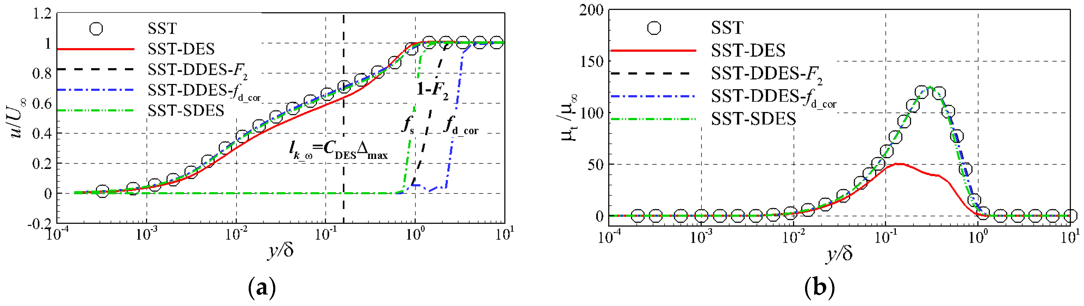
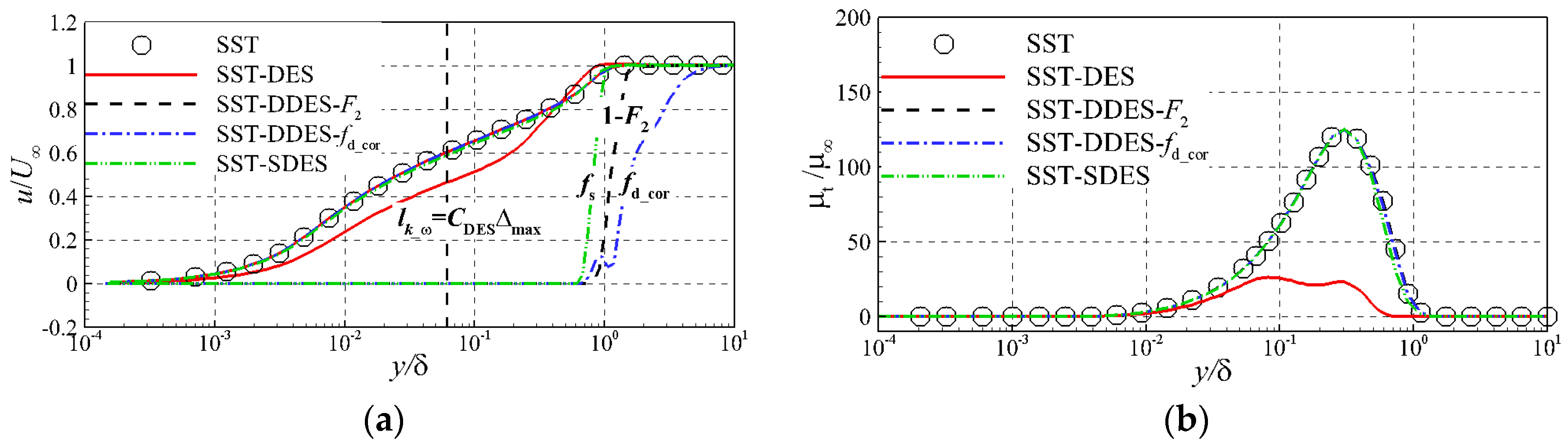
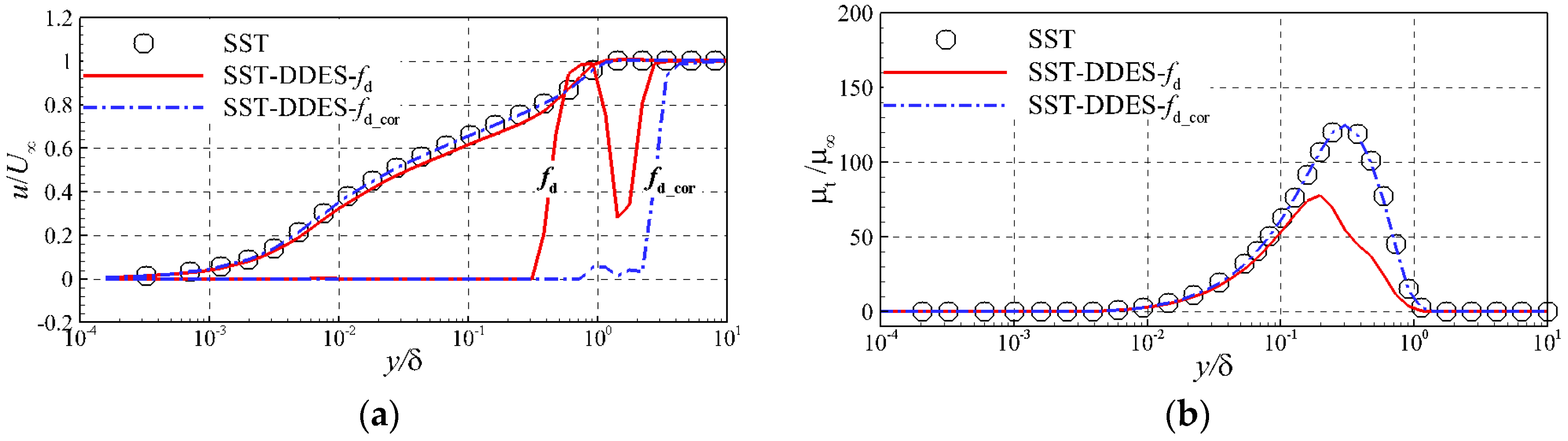
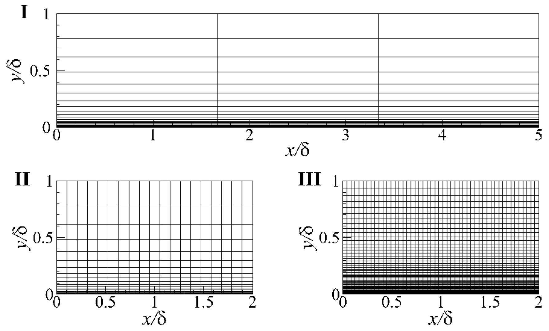
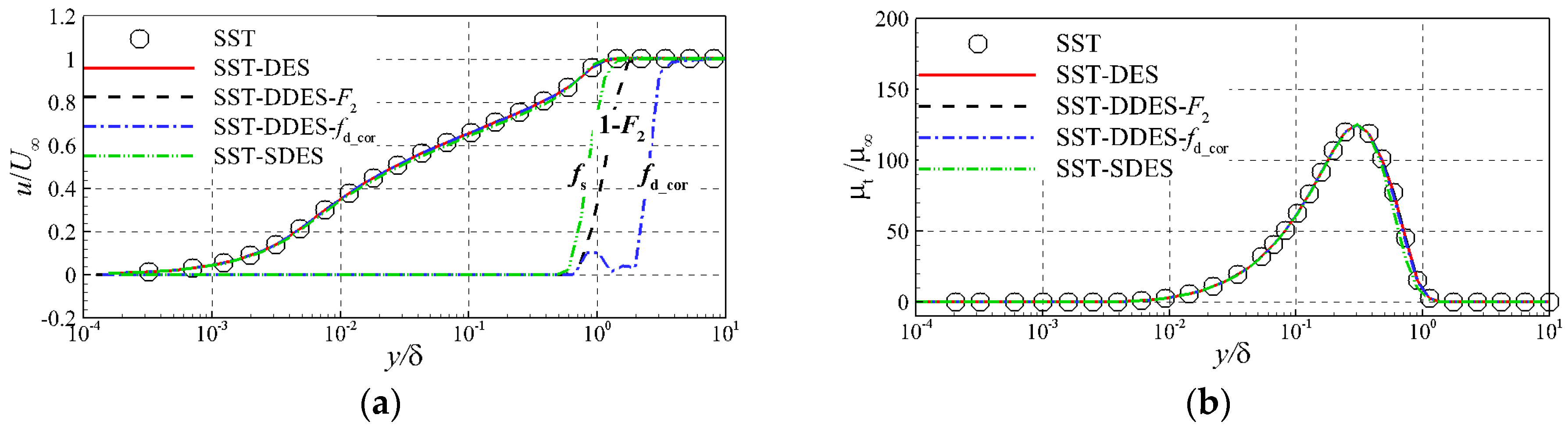
3.1. Flat Plate Flow

The performances of the above DDES methods are preliminarily investigated on a zero-pressure-gradient boundary-layer flow with Re = 2 × 10⁶/m. All cases are computed in RANS mode with the DDES option activated. Similar to the procedure adopted by Reference [7], we also present three types of grids with different mesh resolutions in order to evaluate the grid sensitivity of the above DDES methods. Figure 1 displays the sketch maps of three grid densities in a boundary layer. In a Type I grid, the wall-parallel spacing Δx and Δz set Δ via the max formula and exceed δ, so that the DES length scale is on the “RANS branch” throughout the boundary layer. The shielding functions of DDES methods have no effect in a Type I grid, and all the results are consistent with those of SST (Figure 2). However, the modified shielding function fd_cor turns out to be overly conservative as it covers double the boundary-layer thickness, while both shielding functions F2 (actually 1 − F2 in current notation) and fs accurately denote the whole layer (Figure 2a). Such a conservative shielding function fd_cor will inhibit the main DES functionality by suppressing the LES mode for resolved turbulence. The resolution of Type II grid ranges between the classical values used in LES and RANS simulations (with a target value of the grid-spacing equal to one tenth of the boundary-layer thickness). With this ambiguous grid, the RANS-modeled range (dw < CDESΔ) in SST-DES [18] only holds 18% of the boundary layer (Figure 3a), resulting in underestimating the eddy viscosity by almost 60% (Figure 3b) and the velocity profile slightly departing from that of SST at the log-law region (Figure 3a). This premature switching inside the boundary layer to the LES mode is completely eliminated for all the DDES methods, whereas the performances of the inherent shielding functions are similar to those in a Type I grid (Figure 2a). For a Type III LES grid, all spacings are much smaller than the boundary-layer thickness δ. Since the LES region where CDESΔmax < lk-ω occupies the bulk of the boundary layer, the velocity profile of SST-DES further departs from that of SST, along with the eddy viscosity being underestimated by 87% (Figure 4). All DDES methods could predict consistent results with those of SST. Compared with the performances in Type I and II grids, the modified fd_cor predicts a more accurate range of δ (fd_cor = 0), but rises to 1 more slowly than F2 and fs. Additionally, the original fd is introduced in SST-DDES (SST-DDES-fd) and the results are also shown in Figure 5. The original one increased to be 1 in a much narrower domain (Figure 5a), which results in a less-reliable shielding capability. The SST-DDES-fd underestimates the eddy viscosity by about 40% (Figure 5b). This deficiency was also revealed in References [11,12].
From the discussion above, while the shielding function fd of SA-DDES was considered generic [7], it is essentially calibrated for SA model. When it is applied into the SST-based DDES, the original fd proves to be less reliable, while the recalibrated fd_cor recommended in [11,12] turns out to be much too conservative. Compared with the performance of F2, the entropy function fs increases to 1 more quickly towards the edge of boundary layer, which is favorable for the safe protection of the LES resolved region.

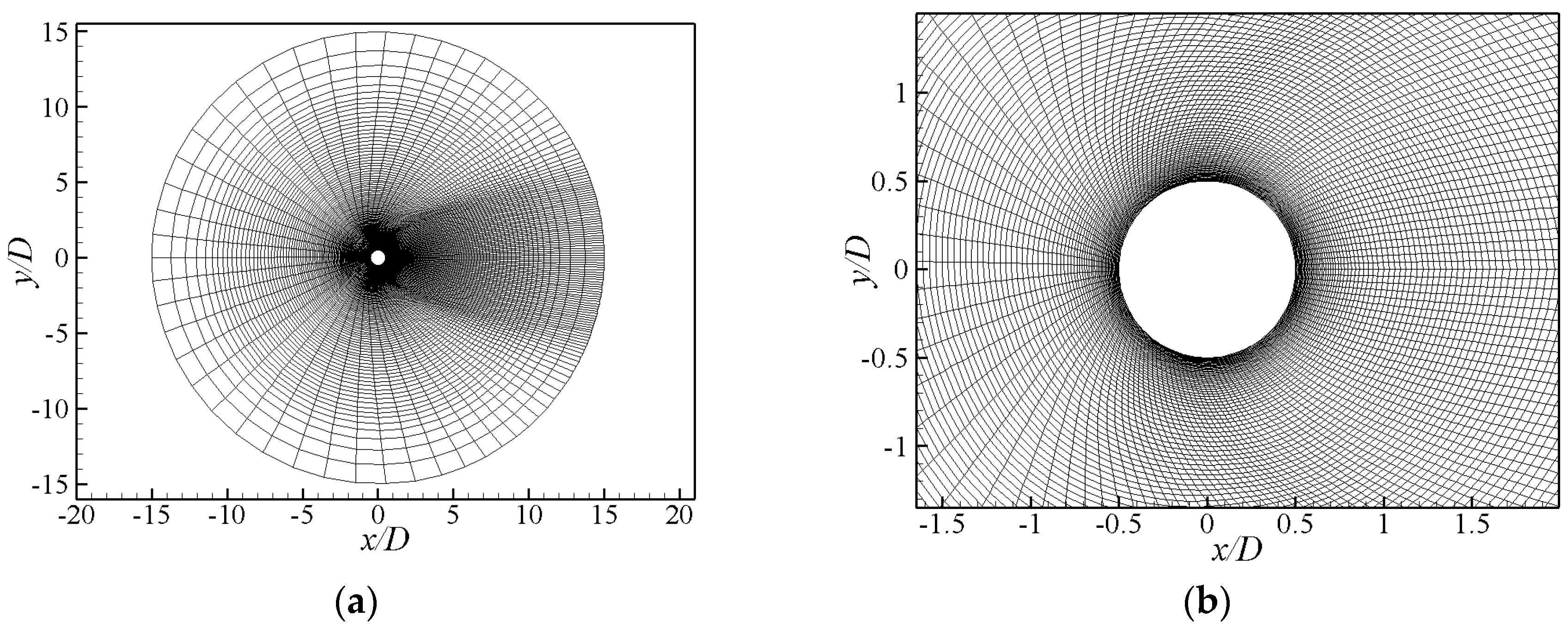
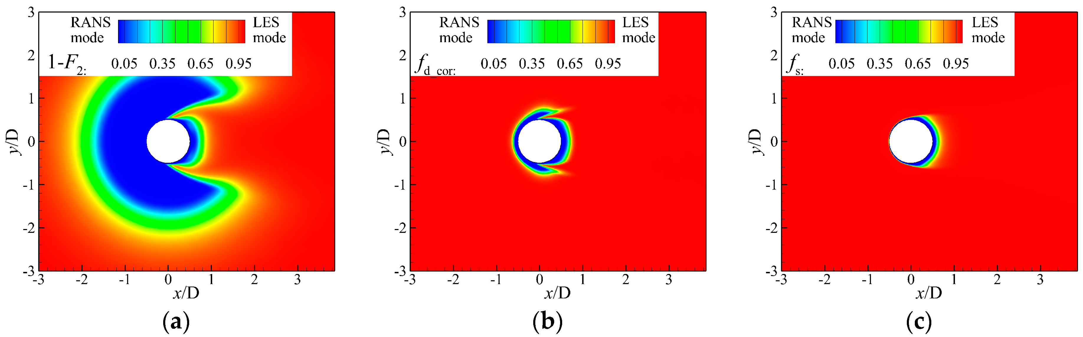
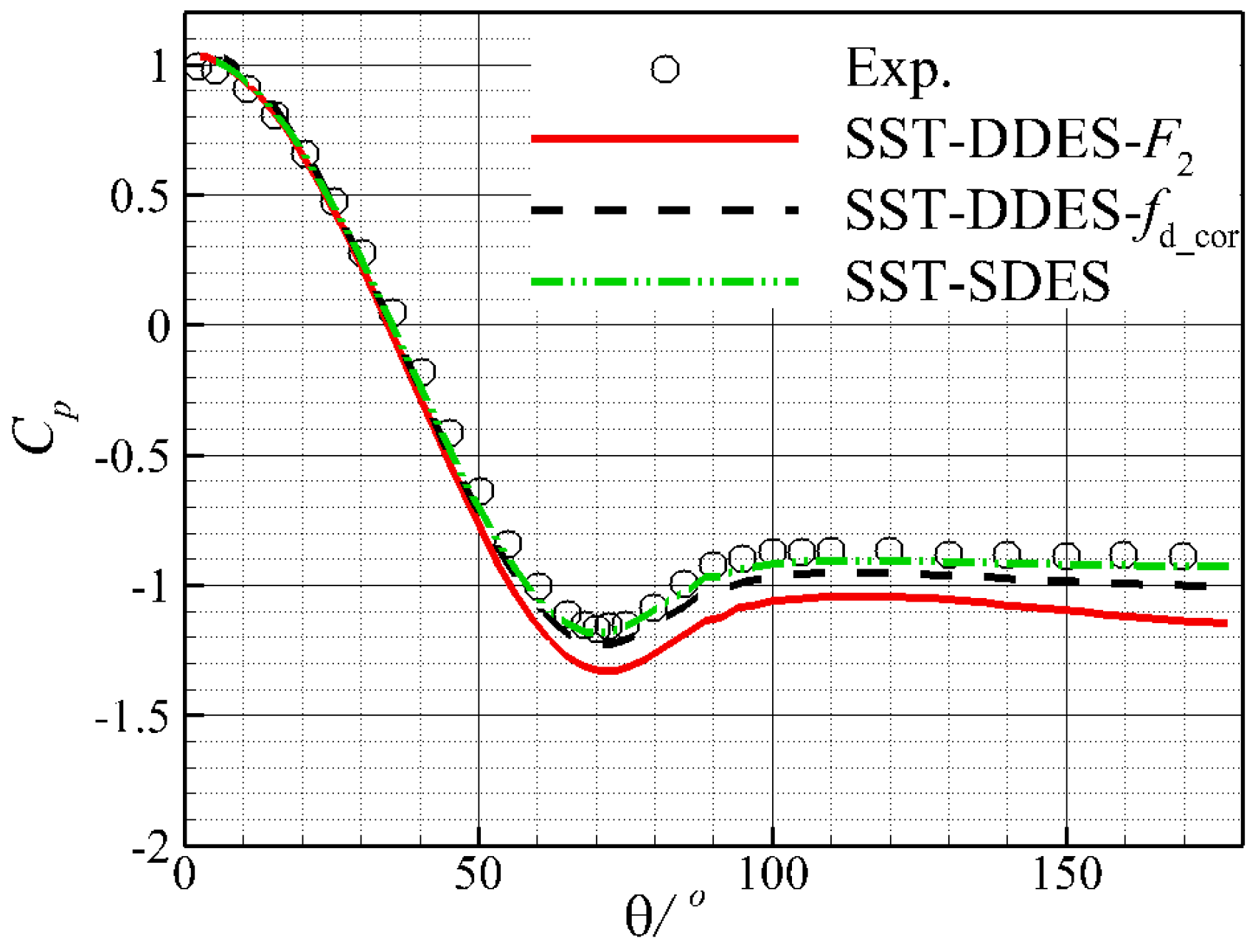
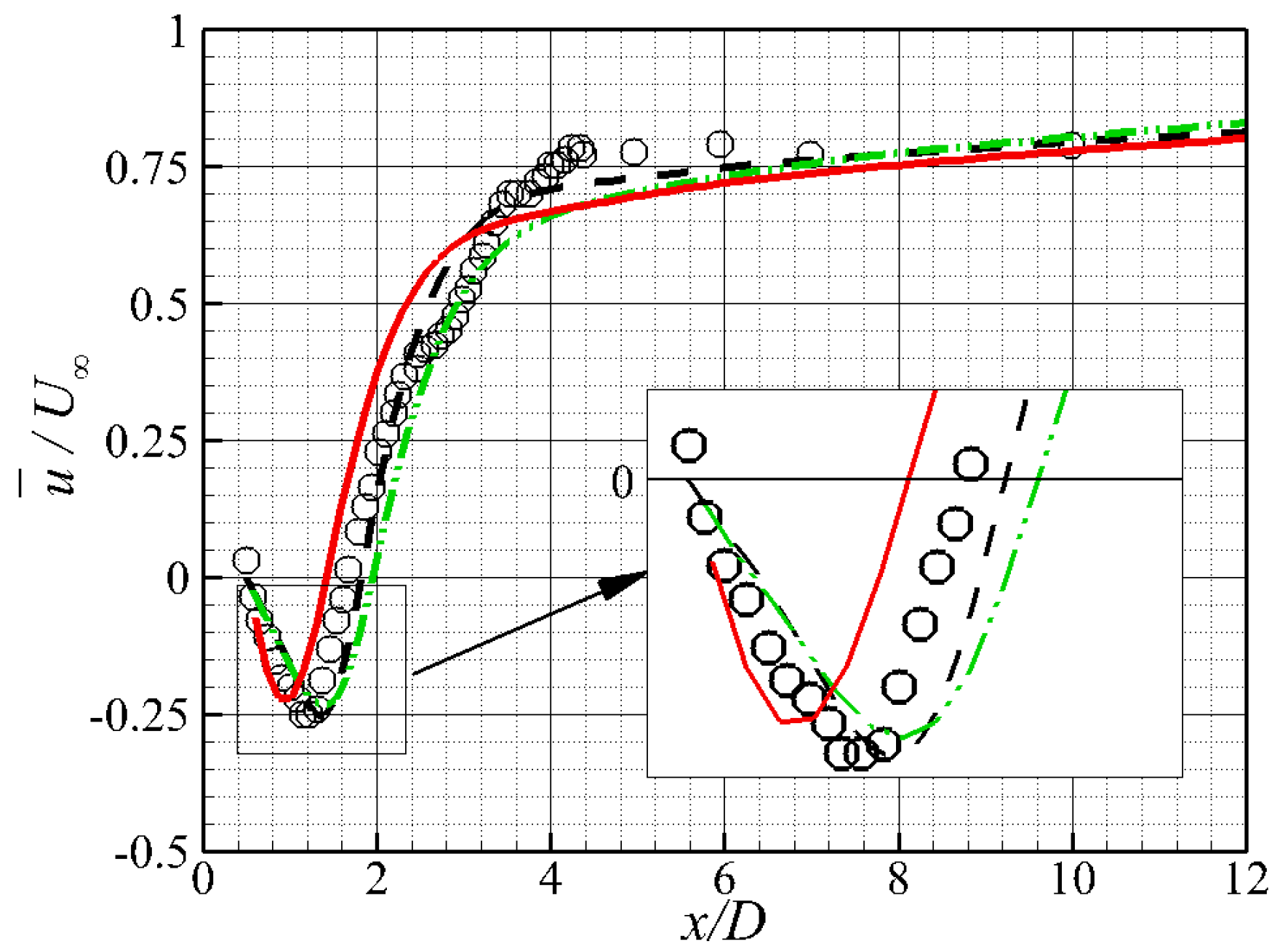
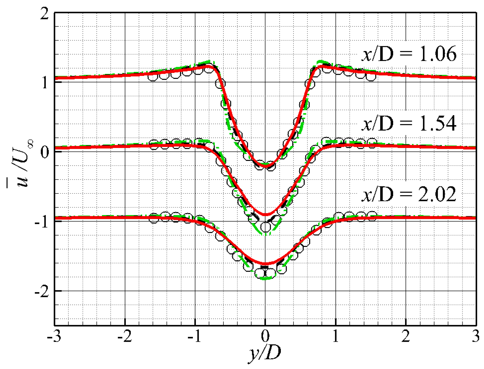
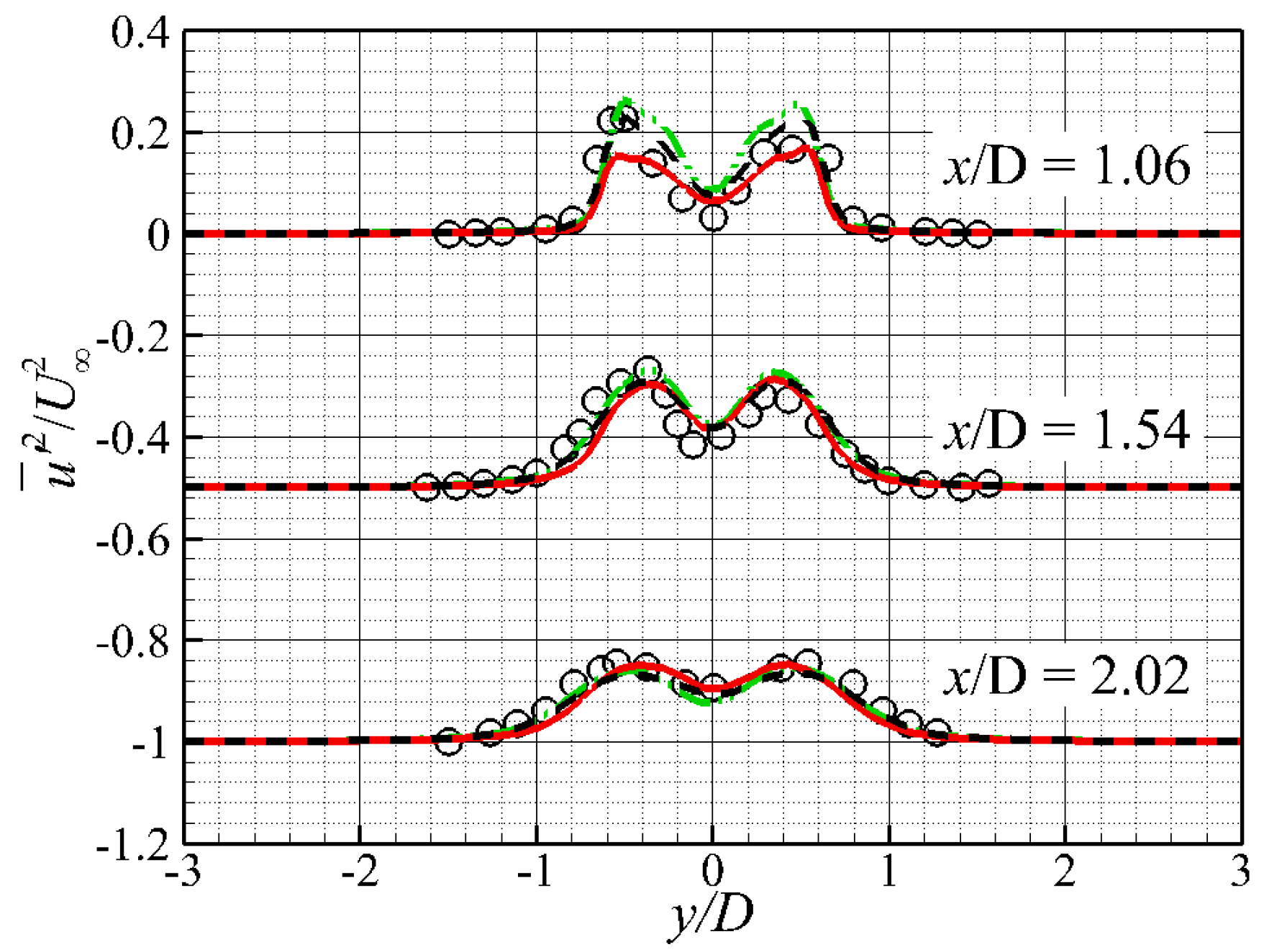
3.2. Circular Cylinder Flow

The flow past a circular cylinder at Reynolds number 3900 based on the cylinder diameter D is chosen for the intended investigations. This kind of large separated flow is considered to be the primary application of DES variants. The size of the integration domain for the O-type grid is 20D in the cross-section plane [22], and the grid extends πD/2 in the z direction (Figure 6). The grid is clustered near the cylinder and the spacing is increased in a proper ratio. The distance of the first grid line to the wall is 10−5, which corresponds to a y+ less than 1.0. The dimensions in the order “streamwise × transverse × spanwise” are 137 × 137 × 41, which had been proved to be refined enough for DES simulations [23]. Periodic boundary condition was employed at the boundaries in the spanwise direction and no-slip boundary condition was prescribed at the surface of cylinders.
Three calculations were carried out on the same grid. The time-averaged distributions of shielding functions in the three DDES methods are compared in Figure 7. As pointed out by Zdravkovich [24], when the Reynolds number varies from 350 to 2 × 10⁵, the flow past a circular cylinder is in the transition-in-shear-layers region, in which the separated boundary layer remains laminar, while a transition takes place along the free-shear layers with shedding vortexes leaving the body as large-scale turbulent vortices. Therefore, a little RANS-modeled region is needed before the separation point. However, both SST-DDES-F2 and -fd_cor preserve an obvious RANS region in front of the cylinder which seems redundant (Figure 7a,b). Comparatively, the shielding function fs employed by SST-SDES is sensitive to the local flow topology and could detect the boundary layer more physically (Figure 7c).
Table 2 presents the values of global flow quantities in all cases and the experiment. According to Bearman [25], the mean recirculation length L ¯ r / D of circular cylinders is inversely proportional to the mean base pressure coefficient C ¯ p b , whereas the mean drag coefficient C ¯ D is proportional to C ¯ p b at subcritical Reynolds numbers. Following this rule, one can easily understand the relationship between Figure 8, Figure 9 and Table 2. As Figure 8 shows, the profile of SST-DDES-F2 is notably below the experimental result, related with the shortest recirculation area (Figure 9) and the largest mean drag coefficient among the three methods (Table 2). Compared with other results, the behavior of SST-DDES-F2 tends to be that of unsteady RANS (URANS) in some sense [18], as it reserved more regions for RANS mode. In contrast, SST-SDES predicts the most convenient results with the experimental data, with the longest recirculation area and the largest Strouhal number. After all, considering the experimental data and LES results with 961 × 960 × 48 grid resolution [26], all three DDES strategies could give convenient mean and fluctuating velocity distributions in the wakes, proving the capability to solve the large-separated flows (Figure 10 Figure 11).

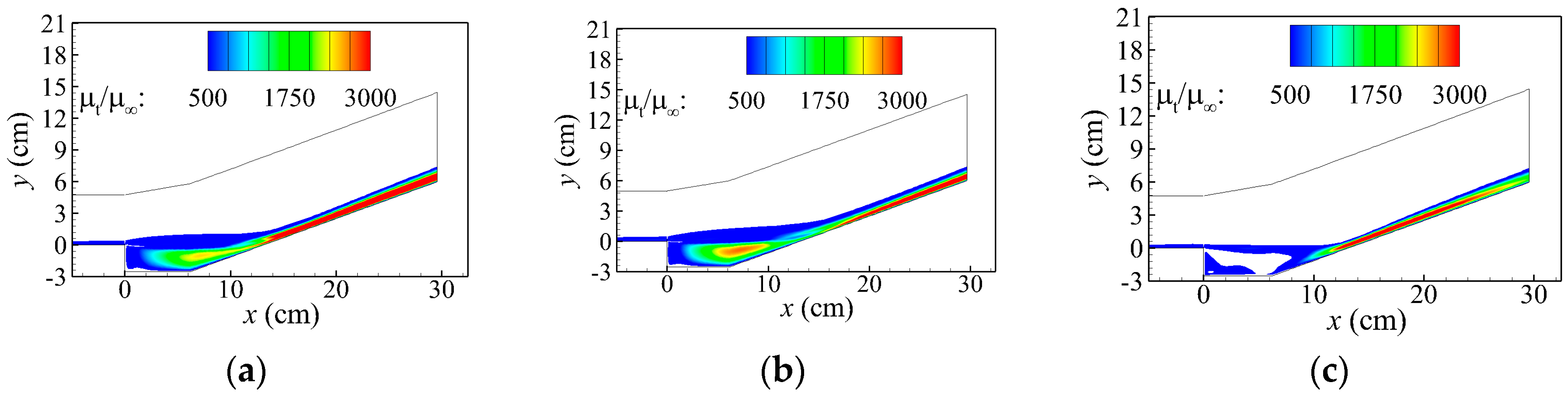
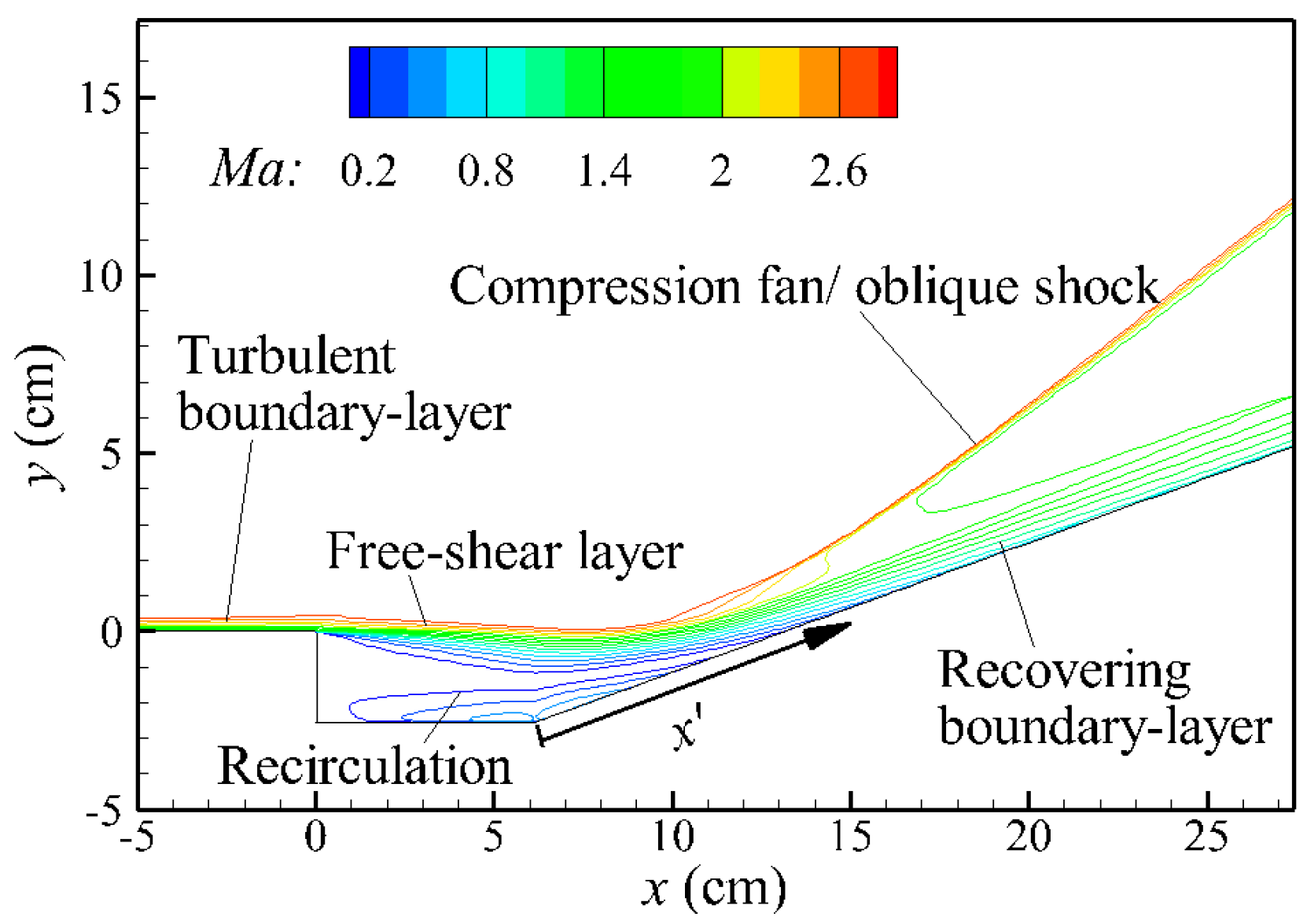
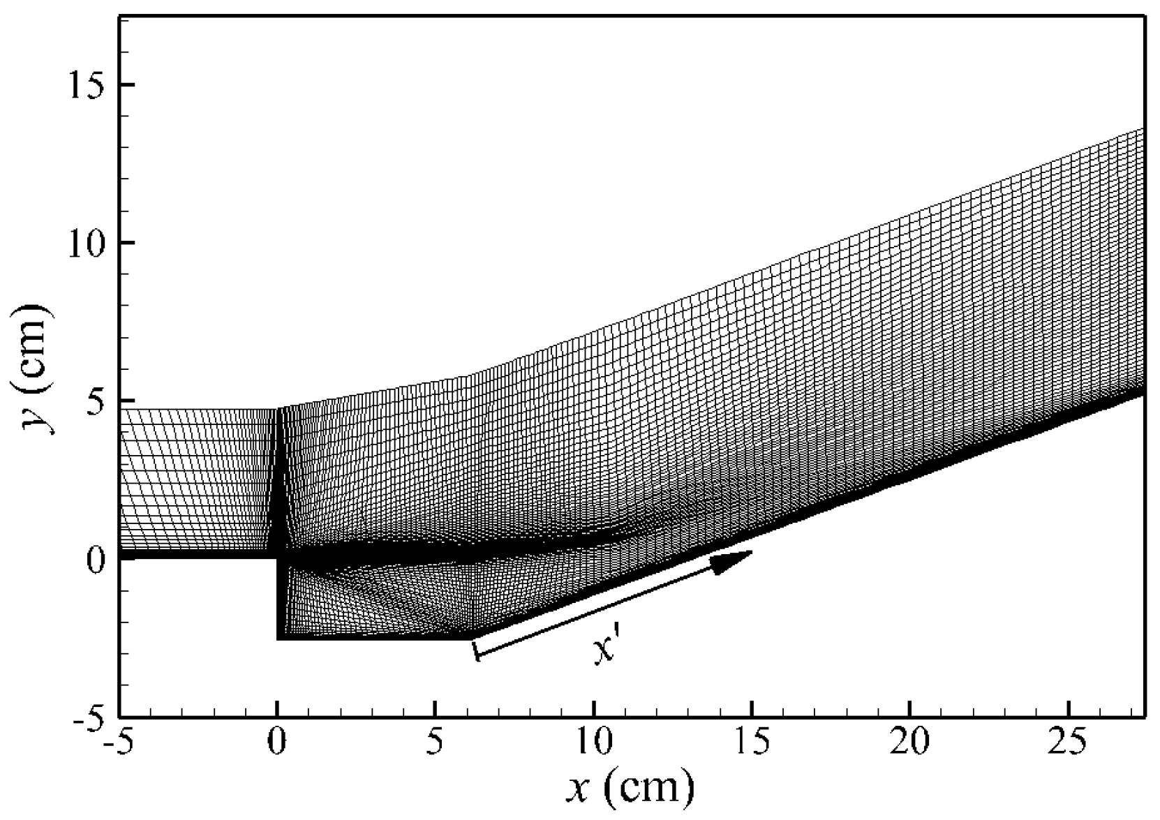
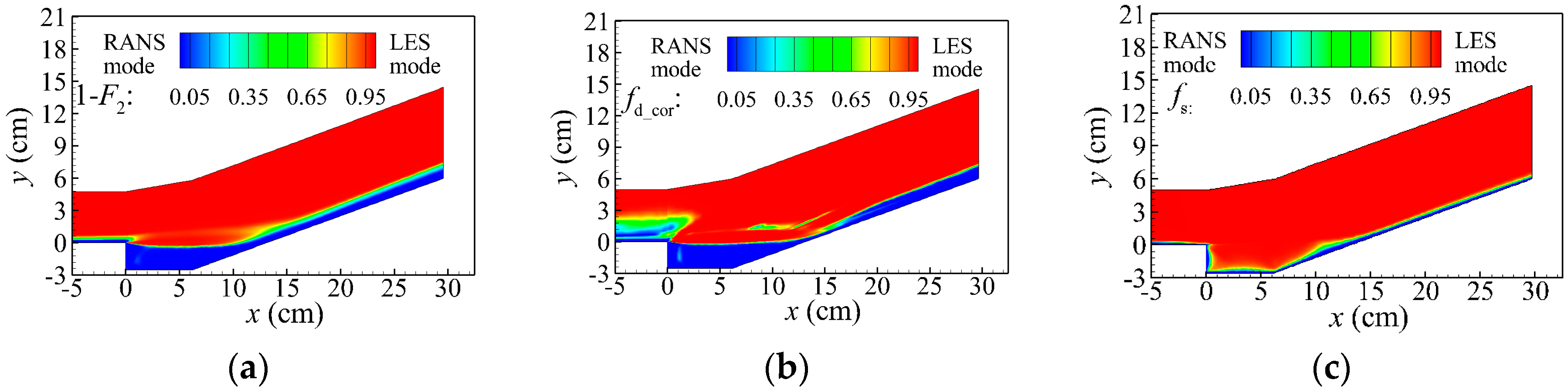
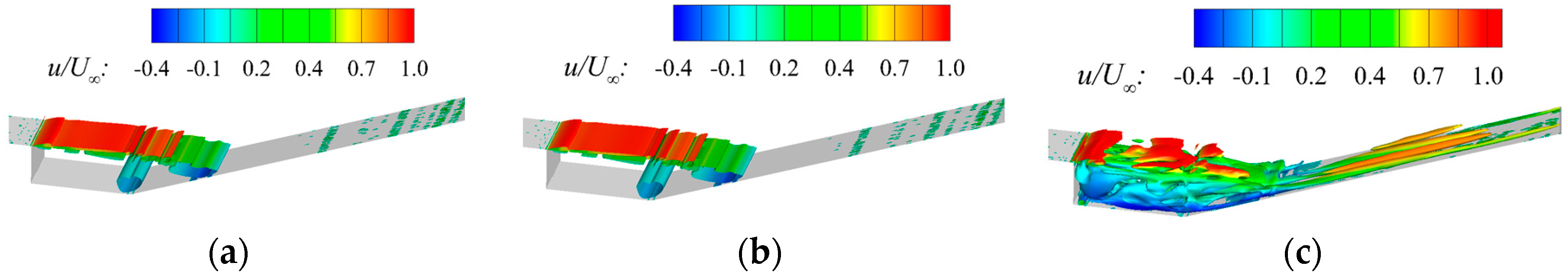
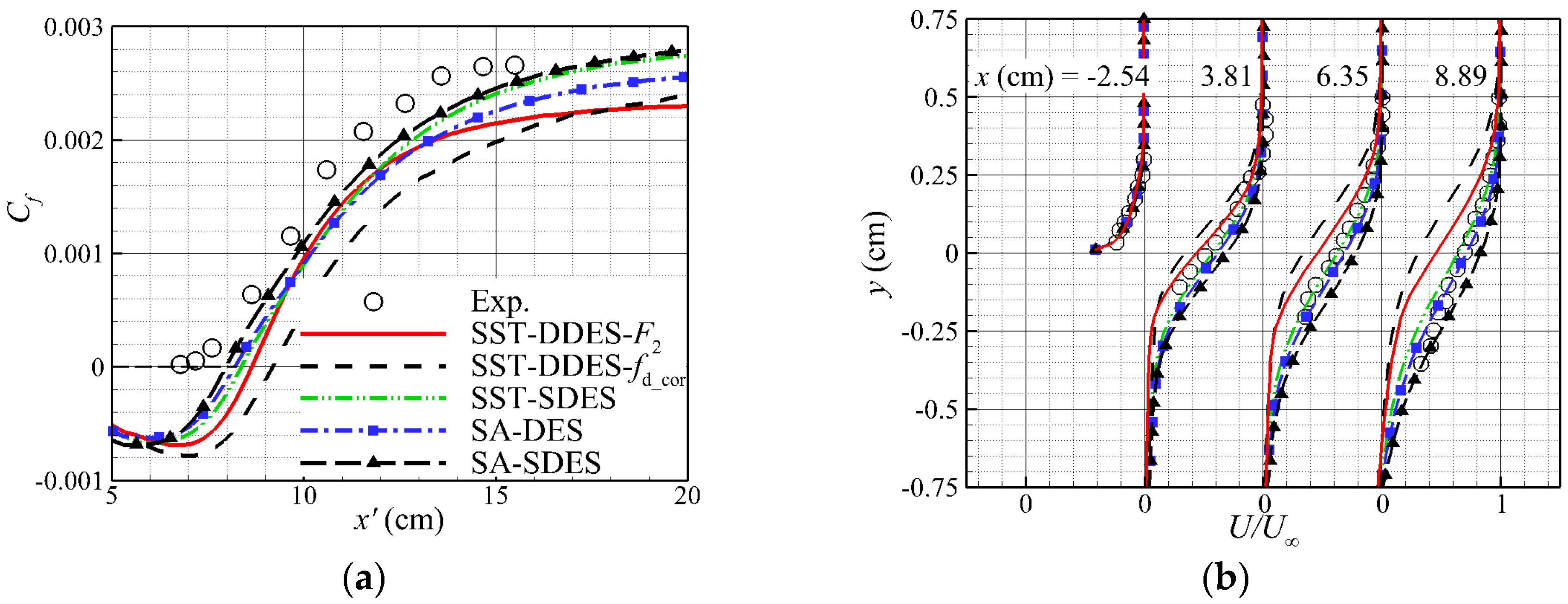
3.3. Cavity-Ramp Flow

The cavity-ramp configuration could be considered as a simplified scramjet or ramjet for the next-generation hypersonic vehicles, which may be used to provide flame stabilization. The dominant features of the flow are the free-shear layer over the cavity and a large recirculation zone behind the cavity leading edge, which should be resolved in LES mode of DES variants. After reattachment, the flow forms the turbulent boundary layer on the ramped portion of the cavity, where the RANS mode is needed (Figure 12). Settles et al. [29] had carried out corresponding experiments, and the nominal inflow Mach number, pressure, and temperature are 2.92, 21,240 Pa, and 95.37 K, respectively. As Figure 13 shows, the three-dimensional grid used for this case consists of two blocks, containing 37 × 85× 33 points upstream of the cavity and 154 × 108 × 33 points downstream of the leading edge of the cavity. The grid was clustered to all solid surfaces, while the free-shear layer and reattachment regions were paid particular attention. It should be noted that this grid resolution is almost the same as Reference [30], which was proved to be refined enough for DES-like methods but were too coarse to properly capture the eddy structure by LES. A no-slip adiabatic condition was applied to the surface, and periodic boundary conditions were employed in the z direction. Initial conditions for DDES simulations are obtained by solving the flowfield with the corresponding RANS model. This case is also employed to evaluate the performances of SA-based DES and SDES [13].
Figure 14 presents the time-averaged distribution of the shielding function inherent in corresponding DDES method. All of the three DDES methods could preserve a visible RANS-modeled region along the wall, whereas both SST-DDES-F2 and -fd_cor mistakenly shield the whole cavity as the boundary layer. Moreover, the inlet distribution of fd_cor fluctuates due to Ui,j ≈ 0 outside of the inflow boundary layer. On the other side, SST-SDES protects a reasonable extent of the boundary layer as RANS mode in the cavity and after the reattachment along the ramp (Figure 14c). Specially, the distribution of entropy function fs of SST-SDES is almost the same as the one inherent in SA-SDES, proving the independence of fs on any particular turbulence model.
Figure 15 compares the time-averaged eddy viscosity distributions of the three DDES methods. Since the cavity is treated in RANS mode by both SST-DDES-F2 and -fd_cor, there are more prominent levels of eddy viscosity than the result of SST-SDES. The entropy function fs reliably indicates the development of the reattached boundary layer along the ramp, resulting in a more reasonable eddy viscosity distribution. The instantaneous vortex structures are visualized in Figure 16, using the Q-criterion. The initial growth of the shear layer is dominated by Kelvin–Helmholtz structures, which are initially two-dimensional, and quickly break down into small vortices in the cavity. After reattachment, elongated horseshoe vortices are observed in the ramp portion, the size of which is on the order of half the domain width in the z direction [30]. Due to the abundant eddy viscosity in the cavity (Figure 15a,b), the turbulent fluctuations inherent in the separated flow are greatly suppressed, leading to fewer vortex structures (Figure 16a,b). However, for SST-SDES, the turbulence-resolving capability in the separation region is not impaired (Figure 16c), as the cavity is indicated as LES mode by entropy function fs.
Figure 17a presents the time-averaged distributions of skin friction coefficient in the recovery region. In addition, the results of SA-based DES and SDES in Reference [13] are also included for comparisons. The x-axis is parallel to the ramp, measured from the juncture of the cavity and the ramp (Figure 12). Among the three DDES methods, the results of SST-SDES are the most consistent with the experiment. Since the rise of skin frication coefficient profile indicates the rate of recovery of the boundary layer downstream of reattachment, fs could denote a comparatively accurate development of the reattached boundary layer. As aforementioned, the friction coefficient distributions are underestimated by SST-DDES-F2 and -fd_cor, due to the lack of turbulent fluctuations resolved by LES mode. Accordingly, the recovering streamwise velocity predicted by SST-SDES develops more quickly than other results, which agrees well with experimental data (Figure 17b). Compared with the three above SST-based DDES methods, SA-DES and SA-SDES tend to predict much more convenient results with the experimental data. The discrepancies may lie in the variant performances of RANS models in adverse-pressure flows [31].

4. Conclusions

A novel version of SST-based DDES, named SST-SDES, was proposed by employing the entropy function fs to shield the turbulent boundary layer as RANS mode. For comparisons, the original SST-DDES-F2 and the recalibrated SST-DDES-fd_cor were also included to interpret their different performances. In the case of turbulent boundary-layer flow, all of the three DDES methods could avoid MSD phenomena. The entropy function fs in SST-SDES accurately indicates the layer range from the point of energy dissipation, while the modified shielding function fd_cor in SST-DDES-fd_cor turns out to be overly conservative as it covers double the boundary-layer thickness. For the circular cylinder flow with fully separation, all three methods could predict consistent results, regarding their mean and instantaneous performances. However, SST-DDES-F2 preserves an obviously redundant RANS region in front of the cylinder. For the cavity-ramp flow with both separation and reattachment, the entropy function fs of SST-SDES protects a reasonable extent of the boundary layer as RANS mode, resulting in the most convenient result with the experiment. Moreover, fs depicts a consistent distribution as the one inherent in SA-SDES, proving its independence on any particular turbulence model. On the downside, both shielding function F2 and fd_cor are so conservative that they suppressed the formation of large-scale turbulent structures in the cavity.
In conclusion, all three DDES methods are capable of dealing with fully-separated flows past bluff bodies. However, for the engineering applications containing flow separations and reattachment, SST-SDES is preferred for the confident shielding function fs, which successfully balances the needs of avoiding the MSD problem and the desire of not impairing the turbulence-resolving capability. Nevertheless, a further recalibration of fd is suggested to be carried out on a more physical basis, when used in an SST-based DDES model.

Acknowledgments

This work was supported by the National Natural Science Foundation of China under Grants No. 11402024, the Civil Aerospace Technology Advanced Research Project and the Excellent Young Scholars Research Fund of the Beijing Institute of Technology.

Author Contributions

Rui Zhao conceived and developed the idea of the study, and all authors developed the calculations, discussed the results and wrote the manuscript. All authors have read and approved the final manuscript.

Conflicts of Interest

The authors declare no conflict of interest.

References

  1. Stefan, S.; Frank, T. Comparison of numerical methods applied to the flow over wall-mounted cubes. Int. J. Heat Fluid Flow 2002, 23, 330–339. [Google Scholar]
  2. Ashton, N.; West, A.; Lardeau, S.; Revell, A. Assessment of RANS and DES methods for realistic automotive models. Comput. Fluids 2016, 128, 1–15. [Google Scholar] [CrossRef]
  3. Liu, J.L.; Niu, J.L. CFD simulation of the wind environment around an isolated high-rise building: An evaluation of SRANS, LES and DES model. Build. Environ. 2016, 95, 91–106. [Google Scholar] [CrossRef]
  4. Riéra, W.; Marty, J.; Castillon, L.; Deck, S. Zonal detached-eddy simulation applied to the tip-clearance flow in an axial compressor. AIAA J. 2016, 54, 2377–2391. [Google Scholar] [CrossRef]
  5. Alam, M.F.; Thompson, D.S.; Walters, D.K. Hybrid Reynolds-Averaged Navier–Stokes/Large-Eddy simulation models for flow around an iced wing. J. Aircr. 2015, 52, 244–256. [Google Scholar] [CrossRef]
  6. Menter, F.R.; Kuntz, M.; Langtry, R. Ten years of industrial experience with the SST turbulence model. Turbul. Heat Mass Transf. 2003, 4, 625–632. [Google Scholar]
  7. Spalart, P.R.; Deck, S.; Shur, M.L.; Squires, K.D.; Strelets, M.K.; Travin, A. A new version of detached-eddy simulation, resistant to ambiguous grid densities. Theor. Comput. Fluid Dyn. 2006, 20, 181–195. [Google Scholar] [CrossRef]
  8. Menter, F.R.; Kuntz, M. Lecture Notes in Applied and Computational Mechanics; Springer: Berlin Heidelberg, Germany, 2004; Volume 19, pp. 339–352. [Google Scholar]
  9. Menter, F.R. Two-equation eddy-viscosity turbulence models for engineering applications. AIAA J. 1994, 32, 1598–1605. [Google Scholar] [CrossRef]
  10. Spalart, P.R.; Allmaras, S.R. A one-equation turbulence model for aerodynamic flows. In Proceedings of the 30th Aerospace Sciences Meeting & Exhibit, Reno, NV, USA, 6–9 January 1992.
  11. Gritskevich, M.S.; Garbaruk, A.V.; Jochen, S.; Menter, F.R. Development of DDES and IDDES formulations for the k-ω shear stress transport model. Flow Turbul. Combust. 2012, 88, 431–449. [Google Scholar] [CrossRef]
  12. Gritskevich, M.S.; Garbaruk, A.V.; Menter, F.R. Fine-tuning of DDES and IDDES formulations to the k-ω shear stress transport model. Prog. Flight Phys. 2013, 5, 23–42. [Google Scholar]
  13. Zhao, R.; Rong, J.L.; Li, X.L. Entropy and its application in turbulence modeling. Chin. Sci. Bull. 2014, 59, 4137–4141. [Google Scholar] [CrossRef]
  14. Zhao, R.; Yan, C.; Li, X.L.; Kong, W.X. Towards an entropy-based detached eddy simulation. Sci. China Phys. Mech. Astron. 2013, 56, 1970–1980. [Google Scholar] [CrossRef]
  15. Nichols, R.H.; Tramel, R.W.; Bunning, P.G. Evaluation of two high-order weighted essentially nonoscillatory schemes. AIAA J. 2008, 46, 3090–3102. [Google Scholar] [CrossRef]
  16. Shen, Y.Q.; Zha, G.C.; Chen, X.Y. High order conservative differencing for viscous terms and the application to vortex-induced vibration flows. J. Comput. Phys. 2009, 228, 8283–8300. [Google Scholar] [CrossRef]
  17. Xiao, Z.X.; Liu, J.; Huang, J.B.; Fu, S. Numerical dissipation effects on massive separation around tandem cylinders. AIAA J. 2012, 50, 1119–1136. [Google Scholar] [CrossRef]
  18. Strelets, M.K. Detached eddy simulation of massively separated flows. In Proceedings of the 39th Aerospace Sciences Meeting & Exhibit, Reno, NV, USA, 8–11 January 2001.
  19. Walsh, J.; Davies, R.D.M.; McEligot, M.D. On the use of entropy to predict boundary layer stability. Entropy 2004, 6, 375–387. [Google Scholar] [CrossRef]
  20. Adeyinka, O.B.; Naterer, G.F. Modeling of entropy production in turbulent flows. J. Fluids Eng. 2004, 126, 893–899. [Google Scholar] [CrossRef]
  21. Scotti, A.; Meneveau, C.; Lilly, D.K. Generalized smagorinsky model for anisotropic grids. Phys. Fluids A 1993, 5, 2306–2308. [Google Scholar] [CrossRef]
  22. Travin, A.; Shur, M.; Spalart, P.R.; Strelets, M. Detached eddy simulation past a circular cylinder. Flow Turbul. Combust. 2000, 63, 293–313. [Google Scholar] [CrossRef]
  23. Zhao, R.; Yan, C. Detailed investigation of detached-eddy simulation for the flow past a circular cylinder at Re = 3900. Appl. Mech. Mater. J. 2012, 401–412. [Google Scholar] [CrossRef]
  24. Zdravkovich, M.M. Flow around Circular Cylinders; Oxford University Press: Oxford, UK, 1997. [Google Scholar]
  25. Bearman, P.W. Investigation of the flow behind a two-dimensional model with a blunt trailing edge and flitted with splitter plates. J. Fluid Mech. 1965, 21, 241–255. [Google Scholar] [CrossRef]
  26. Philippe, P.; Johan, C.; Dominique, H.; Eric, L. Experimental and numerical studies of the flow over a circular cylinder at Reynolds number 3900. Phys. Fluids 2008, 20, 085101. [Google Scholar]
  27. Norberg, C. Effects of Reynolds Number, Low-Intensity Free-Stream Turbulence on the Flow around a Circular Cylinder; Chalmer University of Technology: Gothenberg, Sweden, 1987. [Google Scholar]
  28. Kravchenko, A.G.; Moin, P. Numerical studies of flow over a circular cylinder at ReD = 3900. Phys. Fluids 2000, 12, 403–416. [Google Scholar] [CrossRef]
  29. Settles, G.S.; Williams, D.R.; Baca, B.K.; Bogdonoff, S.M. Reattachment of a compressible turbulent free shear layer. AIAA J. 1982, 20, 60–67. [Google Scholar]
  30. Fan, T.C.; Tian, M.; Edwards, J.R.; Hassan, H.A. Validation of a hybrid Reynolds-Averaged/Large-Eddy simulation method for simulating cavity flameholder configurations. In Proceedings of the 31st AIAA Fluid Dynamics Conference & Exhibit, Anaheim, CA, USA, 11–14 June 2001.
  31. Wilcox, D.C. Turbulence Modeling for CFD, 3rd ed.; DCW Industries: La Canada, CA, USA, 2006. [Google Scholar]
Figure 1. Grids in a boundary layer. Top Type I, natural DES; left Type II, ambiguous spacing; right Type III, LES. δ is the boundary-layer thickness. Assume Δz ≈ Δx.
Entropy 19 00093 g001
Figure 2. Comparisons of SST-based DDES results in Type I grid. (a) Velocity and shielding functions distributions; (b) Eddy viscosity distributions.
Entropy 19 00093 g002
Figure 3. Comparisons of SST-based DDES results in Type II grid. (a) Velocity and shielding functions distributions; (b) Eddy viscosity distributions.
Entropy 19 00093 g003
Figure 4. Comparisons of SST-based DDES results in Type III grid. (a) Velocity and shielding functions distributions; (b) Eddy viscosity distributions.
Entropy 19 00093 g004
Figure 5. Performances of shielding function fd and its corrected version fd_cor on the flat plate flow when applied by SST-based DDES. (a) Velocity and shielding functions distributions; (b) Eddy viscosity distributions.
Entropy 19 00093 g005
Figure 6. X-y grid for circular cylinder at Re = 3900. (a) Global map; (b) Local map around the wall.
Entropy 19 00093 g006
Figure 7. Distributions of corresponding shielding function inherent in SST-based DDES methods around the cylinder wall. (a) 1 − F2 in SST-DDES-F2; (b) fd_cor in SST-DDES-fd_cor; (c) fs in SST-SDES.
Entropy 19 00093 g007
Figure 8. Pressure coefficient around the cylinder surface (Experiment is from Reference [28]).
Entropy 19 00093 g008
Figure 9. Mean streamwise velocity along the centerline (Experiment is from Reference [28]).
Entropy 19 00093 g009
Figure 10. Mean streamwise velocity at three locations in the near wake (Experiment is from Reference [28]).
Entropy 19 00093 g010
Figure 11. Streamwise velocity fluctuations at three locations in the near wake (Experiment is from Reference [26]).
Entropy 19 00093 g011
Figure 12. Flow structures for the cavity-ramp, depicted by time-averaged Mach number contours.
Entropy 19 00093 g012
Figure 13. Grid construction in the x-y plane.
Entropy 19 00093 g013
Figure 14. Distributions of corresponding shielding function inherent in SST-based DDES methods around the cavity-ramp wall. (a) 1 − F2 in SST-DDES-F2; (b) fd_cor in SST-DDES-fd_cor; (c) fs in SST-SDES.
Entropy 19 00093 g014
Figure 15. Comparisons of eddy viscosity distributions of SST-based DDES methods for cavity-ramp flow. (a) SST-DDES-F2; (b) SST-DDES-fd_cor; (c) SST-SDES.
Entropy 19 00093 g015
Figure 16. Isosurface of Q = U2/2H2 highlighting the turbulent structures, flooded by the magnitude of streamwise flow, U: freestream velocity, H: height of the cavity leading edge. (a) SST-DDES-F2; (b) SST-DDES-fd_cor; (c) SST-SDES.
Entropy 19 00093 g016
Figure 17. Time-averaged distributions of flow quantities. (a) skin-frication coefficients along the ramp; (b) velocity profiles in shear layer.
Entropy 19 00093 g017
Table 1. The turbulent length scales in SST-based DDES methods.
StrategiesTurbulent Length Scale
RANS ModeTransition ModeLES Mode
SST-DDES-F2lk-ω-CDESΔmax/(1 − F2)
SST-DDES-fd_corlk-ωlk-ωfd_cor max(0, lk-ωCDESΔmax)CDESΔmax
SST-SDESlk-ωlk-ωfs max(0, lk-ωCDESΔmax)CDESΔmax
Table 2. Global flow quantities computed by four DES strategies.
StrategiesGlobal Flow Quantities
L ¯ r / D C ¯ D St C ¯ p b
SST-DDES-F20.921.180.20311.144
SST-DDES-fd_cor1.051.140.20421.079
SST-SDES1.321.120.20480.957
Experiment [27]1.33 ± 0.050.99 ± 0.050.215 ± 0.0050.88 ± 0.05
L ¯ r : the time-averaged formation length based on the location of zero averaged-velocity, D: cylinder diameter, C ¯ D : time-averaged drag coefficient, St: Strouhal number, C ¯ p b : back-pressure coefficient.

