Leveraging Receiver Message Side Information in Two-Receiver Broadcast Channels: A General Approach †


1
School of Electrical Engineering and Computing, University of Newcastle, Callaghan, New South Wales 2308, Australia
2
This work was presented partially at the 2015 IEEE International Symposium on Information Theory (ISIT), Hong Kong, China, 14–19 June 2015, and the 2016 IEEE International Symposium on Information Theory (ISIT), Barcelona, Spain, 10–15 July 2016.
*
Author to whom correspondence should be addressed.
Entropy 2017, 19(4), 138; https://doi.org/10.3390/e19040138
Submission received: 9 February 2017
/
Revised: 16 March 2017
/
Accepted: 20 March 2017
/
Published: 23 March 2017
(This article belongs to the Special Issue Network Information Theory)
Abstract
:We consider two-receiver broadcast channels where each receiver may know a priori some of the messages requested by the other receiver as receiver message side information (RMSI). We devise a general approach to leverage RMSI in these channels. To this end, we first propose a pre-coding scheme considering the general message setup where each receiver requests both common and private messages and knows a priori part of the private message requested by the other receiver as RMSI. We then construct the transmission scheme of a two-receiver channel with RMSI by applying the proposed pre-coding scheme to the best transmission scheme for the channel without RMSI. To demonstrate the effectiveness of our approach, we apply our pre-coding scheme to three categories of the two-receiver discrete memoryless broadcast channel: (i) channel without state; (ii) channel with states known causally to the transmitter; and (iii) channel with states known non-causally to the transmitter. We then derive a unified inner bound for all three categories. We show that our inner bound is tight for some new cases in each of the three categories, as well as all cases whose capacity region was known previously.
1. Introduction
Communication over wireless channels motivates the study of broadcast channels [1]. In these channels, a transmitter wishes to send a number of messages to multiple receivers via a noisy shared medium, which can also be time-varying due to, for example, fading or interference. The time-varying factor is commonly referred to as the channel state.
The messages to be sent by the transmitter may already be present in parts at some of the receivers, referred to as receiver message side information (RMSI). This form of side information appears in multimedia broadcasting with packet loss. Suppose that a multimedia file is requested by multiple receivers, and the transmission is subject to packet loss. After a few rounds of transmissions, each receiver may a priori know some of the packets re-demanded (due to packet loss) by other receivers. This form of side information appears also in the downlink phase of applications modeled by the multi-way relay channel [2]. For example, consider two stations exchanging data through a satellite. Since each station is also the source of the message to be transmitted by the satellite to the other station in the downlink phase, this phase can be modeled by a broadcast channel with RMSI. As proper use of RMSI may increase transmission rates over broadcast channels, we investigate the capacity region of two-receiver broadcast channels with RMSI. We consider three categories of the two-receiver discrete memoryless broadcast channel: (i) channel without state; (ii) channel with causal channel state information at the transmitter (CSIT) including the cases where the channel state may also be available causally or non-causally at each receiver (It does not make a difference whether the channel state is available causally or non-causally at a receiver. This is due to block decoding, where the receiver decodes its requested message(s) at the end of the channel-output sequence.); and (iii) channel with non-causal CSIT including the cases where the channel state may also be available causally or non-causally at each receiver.
As we will see later, we construct transmission schemes of two-receiver broadcast channels with RMSI using a pre-coding scheme and the best transmission schemes for the channels without RMSI. We here present existing capacity results for the aforementioned three categories of both the two-receiver discrete memoryless broadcast channel without and with RMSI.
1.1. Broadcast Channel without RMSI
1.1.1. Without State
The capacity region is known for several special types of the discrete memoryless broadcast channels, such as the degraded [3], less noisy [4] (p. 121), more capable [5], deterministic [6,7] and semideterministic [8] broadcast channel. The capacity region is also known for the discrete memoryless broadcast channel with degraded message sets (a special message setup where one of the receivers requests only a common message) [9]. Marton’s inner bound with a common message [4] (p. 212) is tight for all cases in this category whose capacity region is known. This inner bound is achieved using superposition coding and Marton coding [4] (p. 207).
1.1.2. With Causal CSIT
Under this category, the capacity region is known for the following two special cases: the degraded broadcast channel with private messages where the channel state is available causally at: (i) only the transmitter [10]; or (ii) the transmitter and the non-degraded receiver [4] (p. 184). Superposition coding and the Shannon strategy [11] were used to characterize the capacity region of these two cases. Superposition coding achieves the capacity region of the degraded broadcast channel without state, and the Shannon strategy is a capacity-achieving strategy for the discrete memoryless point-to-point channel with causal CSIT.
1.1.3. With Non-Causal CSIT
Under this category, the capacity region is known for a few special cases, such as the degraded broadcast channel with private messages where the channel state is available non-causally at the transmitter and the non-degraded receiver [10], and the semideterministic broadcast channel with private messages where the channel state is available non-causally at only the transmitter [12]. Khosravi-Farsani and Marvasti [13] (Theorem 2) used superposition coding, Marton coding and Gelfand–Pinsker coding [14] to derive the best-known inner bound for the discrete memoryless broadcast channel with non-causal CSIT (i.e., it is tight for all cases with known capacity region). Superposition coding plus Marton coding achieves the best-known inner bound for the discrete memoryless broadcast channel without state, and Gelfand–Pinsker coding achieves the capacity region of the discrete memoryless point-to-point channel with non-causal CSIT.
1.2. Broadcast Channel with RMSI
1.2.1. Without State
The capacity region is known for the following three special cases: (i) the discrete memoryless channel with complementary RMSI [15,16] where both receivers need to decode all of the source messages, i.e., all of the messages not known a priori; (ii) the discrete memoryless channel with degraded message sets [17] where one of the receivers needs to decode all of the source messages and one only part of the source messages; and (iii) the less noisy channel with the general message setup [18] (Theorem 3) where each receiver has both common- and private-message requests and knows part of the private message requested by the other receiver.
1.2.2. With Causal CSIT
Under this category, the capacity region is known for the two-receiver discrete memoryless broadcast channel with complementary RMSI where the channel state is available causally at only the transmitter [19].
1.2.3. With Non-Causal CSIT
Under this category, the capacity region is known for the two-receiver discrete memoryless broadcast channel with complementary RMSI where the channel state is available non-causally at the transmitter and one of the receivers [20].
2. Summary of the Main Results
We propose a pre-coding scheme to construct the transmission scheme of a two-receiver broadcast channel with RMSI by applying the pre-coding scheme to the best transmission scheme for the channel without RMSI. We design the pre-coding scheme considering the general message setup where each receiver requests both common and private messages and knows part of the private message requested by the other receiver as RMSI. This provides a general approach for utilizing RMSI in two-receiver broadcast channels. We use our pre-coding scheme and derive a unified inner bound for three categories of the discrete memoryless broadcast channel: (i) channel without state; (ii) channel with causal CSIT (causal category); and (iii) channel with non-causal CSIT (non-causal category). The steps to derive our unified inner bound are shown in Figure 1 in which rectangles with solid sides represent the bounds established in this work. Here, we briefly explain the steps.
Step 1: We first derive an inner bound for the causal category without RMSI. We use superposition coding, Marton coding and the Shannon strategy to construct the transmission scheme. By choosing the common message to be a constant, our scheme reduces to the one used by Kramer [21] for the discrete memoryless broadcast channel without RMSI, with causal CSIT. Our inner bound is tight for all of the cases without RMSI, with causal CSIT, whose capacity region is known (mentioned in the previous section).
Step 2: We then unify our inner bound for the causal category without RMSI, and the best-known inner bound for the non-causal category without RMSI by Khosravi-Farsani and Marvasti [13] (Theorem 2). This result is analogous to the work of Jafar [22] in which a unified capacity-region expression is provided for the point-to-point channel with causal CSIT and the point-to-point channel with non-causal CSIT. Clearly, the capacity region of a non-causal case is larger than or equal to the capacity region of the corresponding causal case (where only the transmitter knows the channel state causally instead of non-causally, and the knowledge of the receivers about the channel state is the same in both cases). This relationship is not necessarily true for their inner bounds especially when one transmission scheme is not a special case of the other. One of the advantages of having a unified inner bound is that it allows us to show that the best-known inner bound ([13] (Theorem 2)) for a non-causal case is larger than or equal to the best inner bound (our inner bound) for the corresponding causal case.
By considering that the channel state is zero with probability one for the channel without state, our unified inner bound reduces to Marton’s inner bound with a common message [4] (p. 212) for the discrete memoryless broadcast channel without state. Consequently, our inner bound covers all three categories without RMSI.
Step 3: Moving on to the channel with RMSI, we propose a pre-coding scheme in order to take RMSI into account. We use our pre-coding scheme in conjunction with the schemes achieving the best inner bounds for the causal and non-causal categories without RMSI, and derive a unified inner bound, which is the best inner bound for all three categories with RMSI. This inner bound reduces to the unified inner bound without RMSI by setting RMSI to zero.
Capacity results: Using our inner bound, we obtain the following new capacity results for the discrete memoryless broadcast channel with RMSI. We also show that our inner bound is tight for all of the cases whose capacity region was known prior to this work. This demonstrates the effectiveness of our proposed approach for utilizing RMSI.
- For the channel with RMSI, without state, we establish the capacity region of two new cases, namely the deterministic channel and the more capable channel. In a concurrent work with the preliminary published version of this work [23], Bracher and Wigger [24] established the capacity region of the semideterministic channel without state for which our inner bound is also tight.
- For the channel with RMSI and causal CSIT, we establish the capacity region of the degraded broadcast channel where the channel state is available causally at: (i) only the transmitter; (ii) the transmitter and the non-degraded receiver; or (iii) the transmitter and both receivers.
- For the channel with RMSI and non-causal CSIT, we establish the capacity region of the degraded broadcast channel where the channel state is available non-causally at: (i) the transmitter and the non-degraded receiver; or (ii) the transmitter and both receivers.
3. System Model
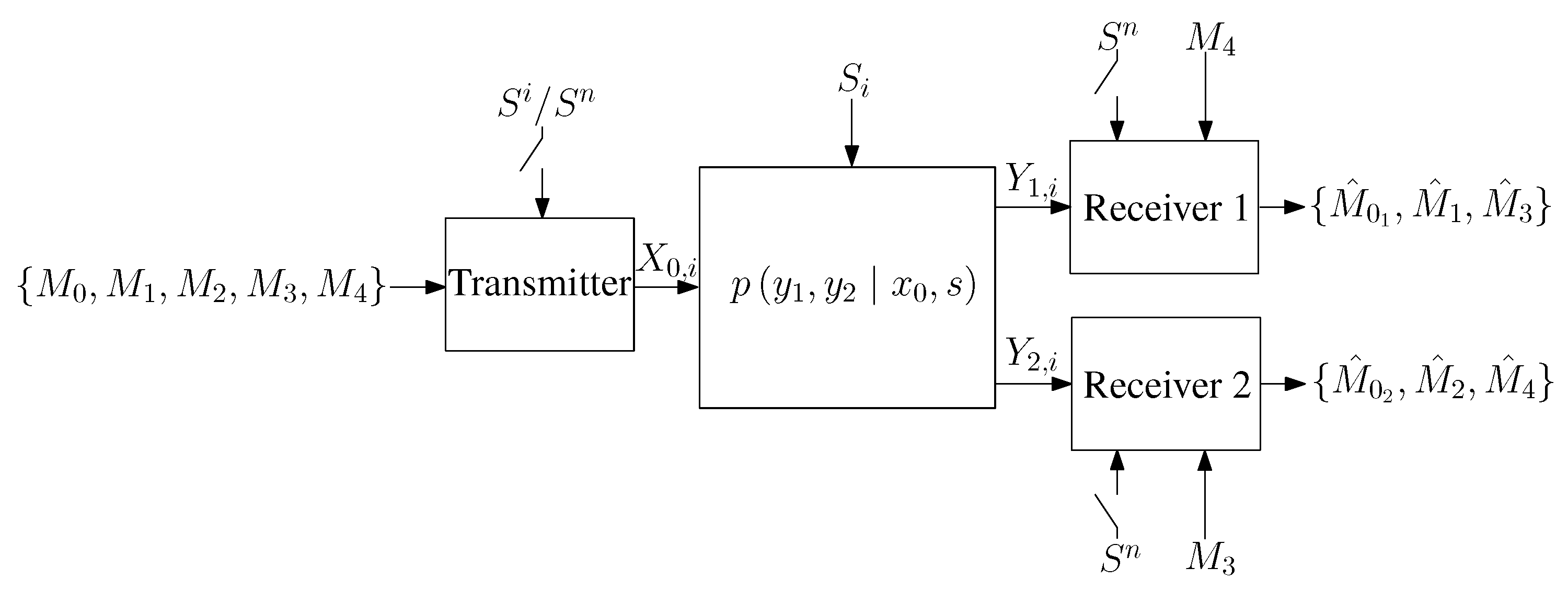
We consider the two-receiver discrete memoryless broadcast channel with independent and identically distributed (i.i.d.) states , depicted in Figure 2, where is the channel input, and are the channel outputs and is the channel state. Considering n uses of the channel, is the transmitted codeword, and , is the channel-output sequence at receiver i.
The source messages are independent, and is uniformly distributed over the set , i.e., transmitted at rate bits per channel use. Receiver 1 requests and knows as RMSI. Receiver 2 requests and knows as RMSI. For Receiver 1, is the part of the private-message request that is not known a priori to the other receiver, and is the part that is known. For Receiver 2, these are and , respectively.
The channel without state is a special case of our channel model by considering , i.e., . This implies that the transmitter and receivers know that the channel state is equal to zero at all channel uses. The channel without RMSI is also a special case of our channel model by considering .
A causal code for the channel consists of a sequence of maps for the encoding:
where × denotes the Cartesian product and denotes the j-fold Cartesian product of , i.e., where . This code also consists of two decoding functions:
where , if the channel state is available at receiver i, and otherwise. is the decoded at Receiver 1, and is the decoded at Receiver 2 where if the channel state is available at receiver i and otherwise.
A non-causal code for the channel consists of an encoding function:
i.e., . This code also consists of two decoding functions, which are defined the same as for the causal code.
A code for the channel without state is defined by choosing in the definition of either the causal code or the non-causal code.
The average probability of error for a code is defined as:
Definition 1.
For causal (non-causal) cases, a rate tuple is said to be achievable for the channel if there exists a sequence of causal (non-causal) codes with as .
Definition 2.
The capacity region of the channel is the closure of the set of all achievable rate tuples .
Definition 3.
The two-receiver discrete memoryless broadcast channel with states is said to be physically degraded if:
and it is said to be stochastically degraded or degraded if there exists a such that form a Markov chain, and we have:
Definition 4.
The two-receiver discrete memoryless broadcast channel without state is said to be deterministic if the channel outputs are deterministic functions of the channel input, i.e., .
Definition 5.
The two-receiver discrete memoryless broadcast channel without state is said to be more capable if for any probability mass function (pmf) .
4. Broadcast Channel without RMSI
In this section, we address the two-receiver discrete memoryless broadcast channel without RMSI, i.e., . We first derive an inner bound for the channel with causal CSIT. We then present the best-known inner bound for the channel with non-causal CSIT [13] (Theorem 2). We finally show that we can have a unified inner bound that covers both causal and non-causal cases, although the achievability schemes are different.
4.1. With Causal CSIT
We utilize superposition coding, Marton coding and the Shannon strategy to derive an inner bound for the discrete memoryless broadcast channel with causal CSIT, stated as Theorem 1.
Theorem 1.
A rate triple for the two-receiver discrete memoryless broadcast channel with causal CSIT is achievable if it satisfies:
for some pmf and some function . if the channel state is available at receiver i and otherwise.
The proof of this theorem is similar to the proof of Marton’s inner bound with a common message [4] (p. 212) for the discrete memoryless broadcast without state. In the encoding, we just need to add the Shannon strategy, and in the decoding, we need to consider instead of as the channel output sequence at receiver i. We here present the proof as we refer to it in Appendix A and in the next section for the channel with RMSI.
Proof of Theorem 1.
(codebook construction) The codebook of the transmission scheme is formed from three sub-codebooks constructed using the pmf . Before constructing the sub-codebooks, using rate splitting, is divided into the two independent messages of rate and of rate , such that . Sub-codebook 0 consists of i.i.d. codewords:
generated according to . Sub-codebook i, , consists of codewords:
generated according to:
where , i.e., for each , codewords are generated.
(Encoding) For the encoding, given , we first find a pair , such that:
where is the set of jointly -typical n-sequences with respect to the considered distribution [4] (p. 29). If there is more than one pair, we arbitrary choose one of them, and if there is no pair, we choose . We then construct the transmitted codeword as , .
(Decoding) Receiver 1 decodes , if it is the unique tuple that satisfies:
otherwise, an error is declared. Receiver 2 similarly decodes , if it is the unique tuple that satisfies:
otherwise, an error is declared. in the decoding is strictly greater than in the encoding.
To derive sufficient conditions for achievability, we assume without loss of generality that the transmitted messages are each equal to one by the symmetry of code construction, and where . Receiver 1 makes an error only if one or more of the following events happen:
Events leading to an error at Receiver 2 are written similarly. Based on the error events and using the packing lemma [4] (p. 45) and the mutual covering lemma [4] (p. 208), sufficient conditions for achievability are:
We finally perform the Fourier–Motzkin elimination to obtain the conditions in (1)–(5). ☐
4.2. With Non-Causal CSIT
Superposition coding, Marton coding and Gelfand–Pinsker coding were used to derive an inner bound for the discrete memoryless broadcast channel with non-causal CSIT [13] (Theorem 2). This inner bound, stated as Proposition 1, is the best-known inner bound for the non-causal category without RMSI.
Proposition 1.
A rate triple for the two-receiver discrete memoryless broadcast channel with non-causal CSIT is achievable if it satisfies:
for some pmf and some function . if the channel state is available at receiver i and otherwise.
Here, we review the scheme achieving this inner bound in order to highlight its differences with the scheme for the channel with causal CSIT.
(Codebook construction) The transmission scheme is formed from three sub-codebooks. These sub-codebooks are constructed using the pmf (i.e., is not independent of S). Before constructing the sub-codebook, using rate splitting, is divided into the two independent messages of rate and of rate , such that . Sub-codebook 0 consists of i.i.d. codewords:
generated according to where , i.e., for each , codewords are generated. Sub-codebook consists of codewords:
generated according to:
where .
(Encoding) For the encoding, given , we first find a triple such that:
If there is more than one triple, we arbitrarily choose one of them, and if there is no triple, we choose . We then construct the transmitted codeword as .
(Decoding) Receiver 1 decodes , if it is the unique tuple that satisfies:
otherwise, an error is declared. Receiver 2 decodes , if it is the unique tuple that satisfies:
otherwise, an error is declared. in the decoding is strictly greater than in the encoding.
4.3. A Unified Inner Bound
Here, we discuss that we can have a unified inner-bound expression for both causal and non-causal cases. The inequalities in (6)–(10) can be used for both the channel with causal CSIT and the channel with non-causal CSIT. This is because, for the channel with causal CSIT, is independent of S, and the terms , , and are zero. Then, the inequalities in (6)–(10) reduce to the ones in (1)–(5), and we can have a unified inner bound, stated as Corollary 1.
Corollary 1.
A rate triple is achievable for the discrete memoryless broadcast channel with causal CSIT if it satisfies (6)–(10) for some pmf and some function . It is achievable for the discrete memoryless broadcast channel with non-causal CSIT if it satisfies (6)–(10) for some pmf and some function .
Remark 1.
This unified inner bound is also the best inner bound for the channel without state. This is because it reduces to Marton’s inner bound with a common message [4] (p. 212) by considering that the channel state is zero with probability one for the channel without state. Therefore, it is a unified inner bound for all three categories without RMSI.
As discussed in Section 2, the capacity region of a non-causal case is larger than or equal to the capacity region of the corresponding causal case. However, an inner bound for a non-causal case is not necessarily larger than an inner bound for the corresponding causal case when the scheme for the latter is not a special case of the scheme for the former. By having a unified inner bound, we can show that the inner bound for a non-causal case (Proposition 1) is larger than or equal to the inner bound for the corresponding causal case (Theorem 1). This is because the domain of the unified inner bound for a causal case (including all pmfs and all functions ) is a subset of the domain of the unified inner bound for the corresponding non-causal case (including all pmfs and all functions ).
In Appendix A, we show that the scheme for the causal category, described in Section 4.1, is not a special case of the scheme for the non-causal category, described in Section 4.2. However, we show that by considering some special cases of the parameters in the scheme for the non-causal category, it asymptotically almost surely has the same codebook construction, encoding and decoding as the scheme for the causal category.
5. Broadcast Channel with RMSI
In this section, we address the two-receiver discrete memoryless broadcast channel with RMSI. We first propose a pre-coding scheme designed to construct the transmission scheme of a channel with RMSI based on the transmission scheme of the channel without RMSI. By applying this pre-coding scheme to the transmission schemes achieving the best inner bounds for the causal and non-causal categories without RMSI, we then derive a unified inner bound that covers all three categories with RMSI. This inner bound includes the unified inner bound for the three categories without RMSI, stated as Corollary 1, as a special case.
5.1. Moving from without RMSI to with RMSI
We construct a pre-coding scheme for a channel with RMSI by considering as a new common message and treating only and as the private messages. , and are then fed to the transmission scheme of the same channel without RMSI. Although Receiver 1 need not decode , having as a part of the common message does not impose any extra constraint. This is because Receiver 1 knows a priori. The same argument applies to for Receiver 2. Since Receiver 1 knows a priori and Receiver 2 knows a priori, Receiver 1 decodes over a set candidates, and Receiver 2 decodes it over a set of candidates.
Conjecture 1.
We conjecture that our pre-coding scheme is an optimal pre-coding scheme in the sense that if a transmission scheme achieves the capacity region of a channel without RMSI, then the transmission scheme, constructed by applying our pre-coding scheme to that transmission scheme, also achieves the capacity region of the same channel with RMSI.
5.2. A Unified Inner Bound
We here present our unified inner bound for the three categories with RMSI, stated as Theorem 2.
Theorem 2.
A rate tuple is achievable for the channel with causal CSIT if it satisfies:
for some pmf and some function . It is achievable for the channel with non-causal CSIT if it satisfies (11)–(15) for some pmf and some function . if the channel state is available at receiver i and otherwise.
Remark 2.
This inner bound is also used for the discrete memoryless broadcast channel with RMSI, without state, where we assume that the channel state is zero with probability one. Therefore, it is a unified inner bound for all three categories with RMSI.
Remark 3.
Having a unified inner bound for the three categories without RMSI and applying the same pre-coding scheme to them are the two basic reasons why we can also have a unified inner bound for the three categories with RMSI.
Proof of Theorem 2.
We prove Theorem 2 by applying our pre-coding scheme to the transmission schemes of the causal and non-causal categories without RMSI.
With causal CSIT: For this category, we apply our pre-coding scheme to the transmission scheme of the discrete memoryless broadcast channel without RMSI, with causal CSIT, described in Section 4.1. Based on our method, Sub-codebook 0 consists of i.i.d. codewords:
generated according to . Sub-codebook i, , consists of codewords:
generated according to:
where .
Encoding and decoding are performed similarly to the case without RMSI. For the encoding, given , we first find a pair , such that:
If there does not exist one pair, we choose . We then construct the transmitted codeword as .
For the decoding, Receiver 1 decodes , if it is the unique tuple that satisfies:
otherwise, an error is declared. Since this receiver knows as side information, it decodes over a set of candidates. Receiver 2 decodes , if it is the unique tuple that satisfies:
otherwise, an error is declared. Since this receiver knows as side information, it decodes over a set of candidates.
Based on error events, written similarly to the case without RMSI and using the packing lemma [4] (p. 45) and the mutual covering lemma [4] (p. 208), sufficient conditions for achievability are:
After performing the Fourier–Motzkin elimination, we obtain Conditions (11)–(15). Note that the terms , , and are zero for this category. The inner bound is computed over all pmfs and all functions .
With non-causal CSIT: For this category, we apply our pre-coding scheme to the transmission scheme of the channel without RMSI, with non-causal CSIT, described in Section 4.2. The resulting changes to the codebook construction, encoding and decoding are similar to the ones for the channel with causal CSIT. Based on error events written similarly to the case without RMSI and using the packing lemma and the multivariate covering lemma [4] (p. 218), sufficient conditions for achievability are:
After performing the Fourier–Motzkin elimination, we obtain Conditions (11)–(15). Note that is not independent of S for this category. The inner bound is computed over all pmfs and all functions . ☐
6. New Capacity Results
In this section, we present new capacity results for the two-receiver discrete memoryless broadcast channel with RMSI. These results are established using our inner bound in Theorem 2. We also show that our inner bound is tight for all of the cases whose capacity region was known prior to this work.
6.1. With RMSI, without State
In this subsection, we first derive a general outer bound for the discrete memoryless broadcast channel with RMSI, without state, stated as Theorem 3. This outer bound is developed based on the Nair-El Gamal outer bound for the discrete memoryless broadcast channel without RMSI, without state [25]. We then establish the capacity region for two new cases in this category: the deterministic channel, stated as Theorem 4, and the more capable channel, stated as Theorem 5.
Theorem 3.
If a rate tuple is achievable for the two-receiver discrete memoryless broadcast channel with RMSI, without state, then it must satisfy:
for some pmf and some function .
Proof of Theorem 3.
See Appendix B ☐
Theorem 4.
The capacity region of the two-receiver deterministic broadcast channel with RMSI, without state, is the closure of the set of all rate tuples , each satisfying:
for some pmf .
Proof of Theorem 4.
(Achievability) Achievability is proven by setting in (11)–(15).
(Converse) We start with the outer bound in Theorem 3. By removing Condition (17), adding Conditions (16) and (21) and enlarging the domain of this outer bound, we obtain the following looser outer bound: if a rate tuple is achievable, then it must satisfy:
for some pmf and some function .
By relaxing Conditions (27)–(31), we can write them in the form of Conditions (22)–(26). As an example, we show this for (31).
where is due to , , for the deterministic channel. ☐
Theorem 5.
The capacity region of the two-receiver more capable broadcast channel with RMSI, without state, is the closure of the set of all rate tuples , each satisfying:
for some pmf .
Proof of Theorem 5.
(Achievability) Achievability is proven by setting in (11)–(15). Note that implies that and .
(Converse) According to Theorem 3, if a rate tuple is achievable, then it must satisfy:
for some pmf and some function . Since, for the channel without state, we have:
and for the more capable channel, we have [4] (p. 123):
we can write (33) and (34) as follows.
From (32), (35), (36) and considering , if a rate tuple is achievable, then it must satisfy:
for some pmf . ☐
6.2. With RMSI, with Causal CSIT
In this subsection, we establish the capacity region of the two-receiver (stochastically) degraded broadcast channel with RMSI where the channel state is available causally: (i) at only the transmitter; (ii) at the transmitter and the non-degraded receiver; or (iii) at the transmitter and both receivers.
Theorem 6.
The capacity region of the two-receiver degraded broadcast channel with RMSI where the channel state is available causally at only the transmitter is the closure of the set of all rate tuples , each satisfying:
for some pmf and some function .
Proof of Theorem 6.
(Achievability) Achievability is proven by setting in (11)–(15). Note that, for a causal case, implies that and . (Converse) See Appendix C. ☐
Theorem 7.
The capacity region of the two-receiver degraded broadcast channel with RMSI where the channel state is available causally either at the transmitter and Receiver 1 or at the transmitter and both receivers is the closure of the set of all rate tuples , each satisfying:
for some pmf and some function . if the channel state is available at Receiver 2 and otherwise.
Proof of Theorem 7.
(Achievability) Achievability is proven by setting in (11)–(15). Note that, for a causal case, implies that , and:
(Converse) See Appendix D. ☐
6.3. With RMSI, with Non-Causal CSIT
In this subsection, we establish the capacity region of the two-receiver (stochastically) degraded broadcast channel with RMSI where the channel state is available non-causally: (i) at the transmitter and the non-degraded receiver; or (ii) at the transmitter and both receivers.
Theorem 8.
The capacity region of the two-receiver degraded broadcast channel with RMSI where the channel state is available non-causally either at the transmitter and Receiver 1 or at the transmitter and both receivers is the closure of the set of all rate tuples , each satisfying:
for some pmf and some function . if the channel state is available at Receiver 2 and otherwise.
Proof of Theorem 8.
(Achievability) Achievability is proven by setting in (11)–(15). Note that, for a non-causal case, implies that , and:
(Converse) See Appendix D. ☐
6.4. Discussion on Prior Known Results
We here show that our inner bound in Theorem 2 is also tight for all of the special cases of the two-receiver discrete memoryless channel with RMSI whose capacity region was known prior to this work.
With RMSI, without state: The capacity region of the discrete memoryless channel with complementary RMSI is achieved by multiplexing all of the requested messages into only one codebook [15,16]. This scheme is a special case of our scheme obtained by setting . Note that and are equal to zero in this message setup.
The capacity region of the discrete memoryless channel with degraded message sets (due to RMSI) is achieved by superposition coding [17]. This scheme is a special case of our scheme obtained by setting or depending on whether Receiver 1 or Receiver 2 needs to decode the whole set of the source messages, respectively. Note that either or is equal to zero in this message setup.
The less noisy broadcast channel with RMSI is a special case of the more capable broadcast channel with RMSI [4]. Thus, our scheme can also achieve the capacity region of the less noisy channel.
With RMSI, with causal CSIT: By setting , our scheme for the causal category reduces to the one used by Khormuji et al. [19] to establish the capacity region of the two-receiver discrete memoryless broadcast channel with complementary RMSI where the channel state is available causally at only the transmitter.
With RMSI, with non-causal CSIT: By setting , our scheme for the non-causal category reduces to the one used by Oechtering and Skoglund [20] to establish the capacity region of the two-receiver discrete memoryless broadcast channel with complementary RMSI where the channel state is available non-causally at the transmitter and one of the receivers.
7. Conclusions
We proposed a pre-coding scheme designed to construct transmission schemes of two-receiver broadcast channels with receiver message side information (RMSI) using the best transmission schemes for the channels without RMSI. This provides a general approach for utilizing RMSI in different two-receiver broadcast channels. Employing our pre-coding scheme, we derived a unified inner bound for three categories of the discrete memoryless broadcast channel with RMSI: (i) channel without state; (ii) channel with causal channel state information at the transmitter (CSIT); and (iii) channel with non-causal CSIT. We showed that our inner bound establishes the capacity region of some new cases in each of the three categories. We also showed that our inner bound is tight for all of the cases whose capacity region was known prior to this work. These results validated our approach for utilizing RMSI in two-receiver broadcast channels.
Acknowledgments
This work is supported by the Australian Research Council under Grants FT110100195, FT140100219 and DP150100903.
Author Contributions
Behzad Asadi developed this work in discussion with Lawrence Ong and Sarah J. Johnson. Behzad Asadi wrote the article with input from Lawrence Ong and Sarah J. Johnson. All authors have read and approved the final manuscript.
Conflicts of Interest
The authors declare no conflict of interest.
Appendix A
In this section, we show that the scheme for the causal category, described in Section 4.1, cannot be considered as a special case of the scheme for the non-causal category, described in Section 4.2. However, the rate regions achievable by both schemes have similar expression. This results in a unified inner bound for both causal and non-causal cases from which we can show that the inner bound for a non-causal case is at least as large as the the inner bound for the corresponding causal case. We will explain the reason behind this observation despite them having different schemes.
We consider a scheme as a special case of another scheme when the latter reduces to the former by considering some special cases of its parameters, e.g., superposition coding is a special case of the scheme achieving Marton’s inner bound with a common message [4] (p. 212).
Consider the encoding rule of the scheme for the non-causal category where the encoder finds a triple , such that:
The encoder for the causal category cannot check this rule since this encoder only knows at the end of the transmission. Hence, the scheme for the causal category is not a special case of the scheme for the non-causal category.
By choosing for all s and setting , the scheme for the non-causal category has the same codebook construction and decoding approach as the scheme for the causal category. The only difference is that for the channel state realization , the encoder for the non-causal category finds a triple , such that:
where:
and the encoder for the causal category finds a triple , such that:
Therefore, the transmitted codewords may be different. However, according to the properties of joint typicality [4] (p. 30), we have:
- .
- For sufficiently large n,
- If , , then, for sufficiently large n,Note that in this item, we have also used the fact that , which results in .
- , as n tends to infinity.
Consequently,
as n tends to infinity. Hence, by choosing , the scheme for the non-causal category asymptomatically almost surely has the same encoding as the scheme for the causal category. This leads the scheme for the non-causal category to achieve the same rate region as the scheme for the causal category.
Appendix B
In this section, we present the proof of Theorem 3, which is based on the proof of the Nair-El Gamal outer bound for the channel without RMSI [4] (p. 217).
Proof.
By Fano’s inequality [4] (p. 19), we have:
where as for . For the sake of simplicity, we use instead of for the remainder.
Using (A1) and (A2), if a rate tuple is achievable, then it must satisfy:
Inequalities (A3)–(A8) yield Conditions (16)–(21) by using the auxiliary random variables defined as:
where and .
We here only show how Inequalities (A3) and (A7) yield Conditions (16) and (20), respectively. We just need to follow similar steps for the rest.
In (A3), we expand the mutual information term as follows
Then, since as , by using the standard time-sharing argument [4] (p. 114), we have:
In (A7), we expand the mutual information terms as follows.
Then, since as , from (A7), (A9), (A10), the Csiszár sum identity [4] (p. 25) and the time-sharing argument, we have:
☐
Appendix C
In this section, we present the converse proof of Theorem 6. In the converse, we assume that the broadcast channel is physically degraded as the capacity region of the stochastically-degraded broadcast channel is equal to its equivalent physically-degraded broadcast channel.
Proof.
(Converse) By Fano’s inequality, we have (A1) and (A2). From (A2) and the physical degradedness of the channel, we have:
and from (A1) and (A11), we have:
Using (A1), (A2) and (A12), we obtain the following necessary conditions for achievability:
We now define the auxiliary random variables and as:
and expand the mutual information terms in (A13)–(A15) respectively as follows.
where follows from the physical degradedness of the channel.
Finally, since as , substituting (A16)–(A18) into (A13)–(A15) and using the time-sharing argument complete the converse proof. Note that is independent of , and is a function of . ☐
Appendix D
In this section, we present the converse proof of Theorems 7 and 8. We here also assume that the broadcast channel is physically degraded.
Proof.
(Converse) By Fano’s inequality, we have:
where as .
From (A20) and the physical degradedness of the channel, we have:
and from (A19) and (A21), we have:
Using (A19), (A20) and (A22), if a rate tuple is achievable, then it must satisfy:
We now define the auxiliary random variables and as:
and expand the mutual information terms in (A23)–(A25) respectively as follows.
where and follow from the physical degradedness of the channel, from the Csiszár sum identity and from the independence of and . Note that, for causal cases, is independent of , but for non-causal cases, and are dependent. For both causal and non-causal cases, is a function of .
Finally, since as , substituting (A26)–(A28) into (A23)–(A25) and using the time sharing argument complete the converse proof. ☐
References
- Cover, T.M. Broadcast channels. IEEE Trans. Inf. Theory 1972, 18, 2–14. [Google Scholar] [CrossRef]
- Ong, L.; Kellett, C.M.; Johnson, S.J. On the equal-rate capacity of the AWGN multiway relay channel. IEEE Trans. Inf. Theory 2012, 58, 5761–5769. [Google Scholar] [CrossRef]
- Gallager, R.G. Capacity and coding for degraded broadcast channels. Probl. Inf. Transm. 1974, 10, 3–14. [Google Scholar]
- El Gamal, A.; Kim, Y.H. Network Information Theory; Cambridge University Press: Cambridge, UK, 2011. [Google Scholar]
- El Gamal, A. The capacity of a class of broadcast channels. IEEE Trans. Inf. Theory 1979, 25, 166–169. [Google Scholar] [CrossRef]
- Pinsker, M.S. Capacity of noiseless broadcast channels. Probl. Inf. Transm. 1978, 14, 28–34. [Google Scholar]
- Han, T.S. The capacity region for the deterministic broadcast channel with a common message. IEEE Trans. Inf. Theory 1981, 27, 122–125. [Google Scholar]
- Marton, K. A coding theorem for the discrete memoryless broadcast channel. IEEE Trans. Inf. Theory 1979, 25, 306–311. [Google Scholar] [CrossRef]
- Körner, J.; Marton, K. General broadcast channels with degraded message sets. IEEE Trans. Inf. Theory 1977, 23, 60–64. [Google Scholar] [CrossRef]
- Steinberg, Y. Coding for the degraded broadcast channel with random parameters, with causal and noncausal side information. IEEE Trans. Inf. Theory 2005, 51, 2867–2877. [Google Scholar] [CrossRef]
- Shannon, C. Channels with side information at the transmitter. IBM J. Res. Dev. 1958, 2, 289–293. [Google Scholar] [CrossRef]
- Lapidoth, A.; Wang, L. The state-dependent semideterministic broadcast channel. IEEE Trans. Inf. Theory 2013, 59, 2242–2251. [Google Scholar] [CrossRef]
- Khosravi-Farsani, R.; Marvasti, F. Capacity bounds for multiuser channels with non-causal channel state information at the transmitters. In Proceedings of the IEEE Information Theory Workshop (ITW), Paraty, Brazil, 16–20 October 2011. [Google Scholar]
- Gel’fand, S.I.; Pinsker, M.S. Coding for channel with random parameters. Probl. Control Inf. Theory 1980, 9, 19–31. [Google Scholar]
- Oechtering, T.J.; Schnurr, C.; Bjelakovic, I.; Boche, H. Broadcast capacity region of two-phase bidirectional relaying. IEEE Trans. Inf. Theory 2008, 54, 454–458. [Google Scholar] [CrossRef]
- Tuncel, E. Slepian–Wolf coding over broadcast channels. IEEE Trans. Inf. Theory 2006, 52, 1469–1482. [Google Scholar] [CrossRef]
- Kramer, G.; Shamai, S. Capacity for classes of broadcast channels with receiver side information. In Proceedings of the IEEE Information Theory Workshop (ITW), Lake Tahoe, CA, USA, 2–6 September 2007. [Google Scholar]
- Oechtering, T.J.; Wigger, M.; Timo, R. Broadcast capacity regions with three receivers and message cognition. In Proceedings of the IEEE International Symposium on Information Theory (ISIT), Cambridge, MA, USA, 1–6 July 2012. [Google Scholar]
- Khormuji, M.N.; Oechtering, T.J.; Skoglund, M. Capacity region of the bidirectional broadcast channel with causal channel state information. In Proceedings of the Tenth International Symposium on Wireless Communication Systems (ISWCS), Ilmenau, Germany, 27–30 August 2013. [Google Scholar]
- Oechtering, T.J.; Skoglund, M. Bidirectional broadcast channel with random states noncausally known at the encoder. IEEE Trans. Inf. Theory 2013, 59, 64–75. [Google Scholar] [CrossRef]
- Kramer, G. Information networks with in-block memory. IEEE Trans. Inf. Theory 2014, 60, 2105–2120. [Google Scholar] [CrossRef]
- Jafar, S. Capacity with causal and noncausal side information: A unified view. IEEE Trans. Inf. Theory 2006, 52, 5468–5474. [Google Scholar] [CrossRef]
- Asadi, B.; Ong, L.; Johnson, S.J. A unified scheme for two-receiver broadcast channels with receiver message side information. In Proceedings of the IEEE International Symposium on Information Theory (ISIT), Hong Kong, China, 14–19 June 2015. [Google Scholar]
- Bracher, A.; Wigger, M. Feedback and partial message side-information on the semideterministic broadcast channel. In Proceedings of the IEEE International Symposium on Information Theory (ISIT), Hong Kong, China, 14–19 June 2015. [Google Scholar]
- Nair, C.; El Gamal, A. An outer bound to the capacity region of the broadcast channel. IEEE Trans. Inf. Theory 2007, 53, 350–355. [Google Scholar] [CrossRef]
Figure 1.
The steps to derive our unified inner bound (the rightmost rectangle) for the three categories: (i) channel with receiver message side information (RMSI), without state; (ii) channel with RMSI and causal channel state information at the transmitter (CSIT); and (iii) channel with RMSI and non-causal CSIT. The rectangles with dashed sides represent the bounds derived prior to this work (i.e., Marton’s inner bound with a common message [4] and non-causal CSIT inner bound [13]). The rectangles with solid sides represent the bounds derived in this work. The arrows provide the key techniques to derive each bound.
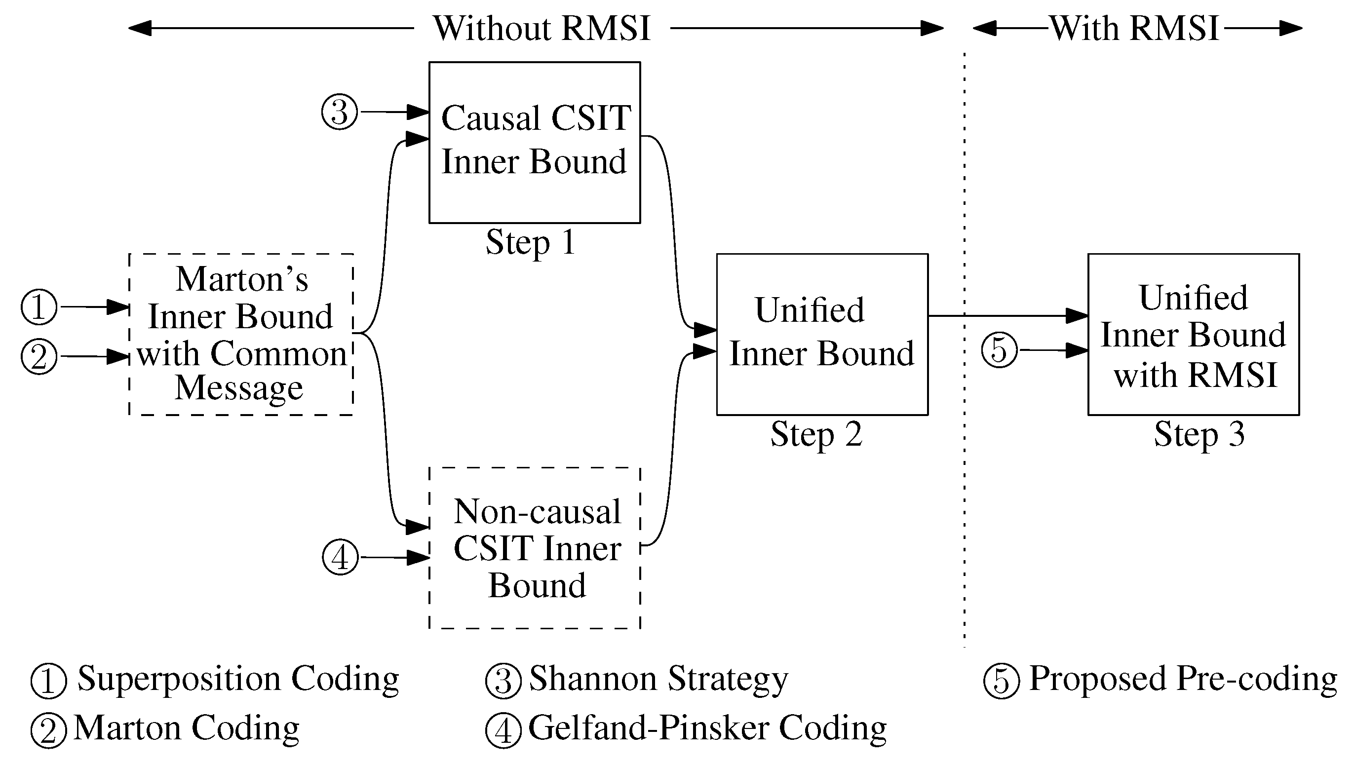
Figure 2.
The two-receiver discrete memoryless broadcast channel with i.i.d. states where the channel state may be available either causally or non-causally at each of the transmitter and receivers. Receiver 1 requests while it knows as side information. Receiver 2 requests while it knows as side information. is the decoded version of at Receiver 1, and is the decoded version of at Receiver 2.

© 2017 by the authors. Licensee MDPI, Basel, Switzerland. This article is an open access article distributed under the terms and conditions of the Creative Commons Attribution (CC BY) license (http://creativecommons.org/licenses/by/4.0/).
Share and Cite
MDPI and ACS Style
Asadi, B.; Ong, L.; Johnson, S.J. Leveraging Receiver Message Side Information in Two-Receiver Broadcast Channels: A General Approach †. Entropy 2017, 19, 138. https://doi.org/10.3390/e19040138
AMA Style
Asadi B, Ong L, Johnson SJ. Leveraging Receiver Message Side Information in Two-Receiver Broadcast Channels: A General Approach †. Entropy. 2017; 19(4):138. https://doi.org/10.3390/e19040138
Chicago/Turabian StyleAsadi, Behzad, Lawrence Ong, and Sarah J. Johnson. 2017. "Leveraging Receiver Message Side Information in Two-Receiver Broadcast Channels: A General Approach †" Entropy 19, no. 4: 138. https://doi.org/10.3390/e19040138
Note that from the first issue of 2016, this journal uses article numbers instead of page numbers. See further details here.