
Minimum Sample Size for Reliable Causal Inference Using Transfer Entropy

National Institute for Space Research, São José dos Campos 12227-010, Brazil
*
Author to whom correspondence should be addressed.
Entropy 2017, 19(4), 150; https://doi.org/10.3390/e19040150
Submission received: 20 February 2017
/
Revised: 29 March 2017
/
Accepted: 29 March 2017
/
Published: 31 March 2017
(This article belongs to the Special Issue Complex Systems and Fractional Dynamics)
Abstract
:Transfer Entropy has been applied to experimental datasets to unveil causality between variables. In particular, its application to non-stationary systems has posed a great challenge due to restrictions on the sample size. Here, we have investigated the minimum sample size that produces a reliable causal inference. The methodology has been applied to two prototypical models: the linear model autoregressive-moving average and the non-linear logistic map. The relationship between the Transfer Entropy value and the sample size has been systematically examined. Additionally, we have shown the dependence of the reliable sample size and the strength of coupling between the variables. Our methodology offers a realistic lower bound for the sample size to produce a reliable outcome.
1. Introduction
Transfer Entropy (TE) [1] is an information-theoretical functional able to detect a causal association between two variables [2,3,4,5]. TE identifies the potential driver and driven variable by statistically quantifying the flow of information from one to the other distinguishing the directionality due to its asymmetric property. Backshifting one variable at some particular lag, it returns a nonzero value indicating information flow between variables, or zero otherwise. However, in real data application, it may assume a nonzero value simply due to bias associated with the finiteness of the sample, and not because of an actual coupling [6,7].
Recently, sophisticated algorithms using transfer entropy have improved causal detection [8,9]. However, even these advanced methods require sufficient sample points to avoid false positives due to data-shortage bias. Previous studies addressed the entropy bias by estimating the probability distribution of the underlying processes [10,11,12]. However, from an inference-based approach, there is still a lack of rigorous computation regarding the appropriate minimum size of the sample for a reliable TE outcome. To overcome such an issue, a statistical hypothesis test is required to distinguish independence from a causal relation. The outcome of testing depends on the sample size. This raises concern regarding the minimum sample size required for TE to provide a reliable inference of causal relation.
To answer this, we employ TE as a statistical test and search for the lower bound of the sample size that produces a reliable true positive. For the purpose of consistency, the investigation is carried out in a stationary regime, so the sample range does not result in a different interaction behavior. To this end, paradigmatic models are used in the analysis: two coupled linear autoregressive-moving-average (ARMA) models and two coupled non-linear logistic maps. The former is used in model-driven approaches to detect Granger causality through parametric estimation [13]. The latter is a typical example of a nonlinear system that challenges causal inference due to its chaotic properties.
The results show that the minimum sample size for reliable outcome depends on the strength of the coupling. The larger the coupling, the smaller the sample size required to provide a reliable true positive. The relationship between coupling strength and sample size varies according to the model. We pinpoint the lower bound of the sample size at the limit of high coupling for each model.
2. Models
The models are constructed to describe two coupled variables X and Y; X influences Y after a lag , with coupling strength regulated by the parameter . In the following subsection, the models are defined.
2.1. Coupled ARMA[p,q]
The ARMA model is a linear regression model used as a toolkit in the Granger causality approach. Two coupled ARMA[] models X and Y are defined; X influences Y after time steps, that is,
where so that n is much bigger than any sample size N; is a uniformly distributed random number; and are parameters that regulate the state transition and stochasticity respectively; finally, is the coupling parameter. For , the two variables are uncoupled, while if , the Y variable is completely defined by X. The parameter is fixed throughout the whole analysis. In the methodology section, we investigate the role of and in detecting .
2.2. Couple Logistic Maps
Inspired by the studies of both Gyllenber [14] and Hastings [15] to describe migration dynamics within two populations, we define the coupled logistic maps with delay as follows
The dynamics of X is the standard logistic map, and the dynamics of Y has two terms. The first is a local logistic growing rate, while the other represents a migration effect, where individuals from the X migrate to Y after time steps. We assume that both populations have the same growth rate . The parameter is the coupling between X and Y and represents the migration influx controlling the growth of one population to the detriment of the other.
3. Methodology
Consider two given sets of discrete variable and . Any causal relationship between them should be restrained in the temporal order of the X and Y elements. Let us suppose that X influences Y after units of time. One can detect this relationship using the TE functional. TE evaluates the reduction in the uncertainty of the past of a possible driver due to the knowledge of the present of a possible driven Y when the past of is given. Figure 1 illustrates the idea behind the sampling for TE calculation. The TE from X to Y is evaluated as follows
Whenever X and Y are infinite independent random variables, the expression (3) is zero. However, in the case of two finite datasets, TE will be greater than zero, even if X and Y are supposed to be independent. This bias is due to a finite size effect, and it has to be addressed via a statistical inference procedure.
Let us assume a null hypothesis stating that X and Y are independent for a particular lag . At this lag, an ensemble of surrogate data is generated from the original data. A confidence interval is defined as a percentile of the surrogate’s TE distribution. If the TE calculated from the original dataset (original TE) is significantly higher than the confidence interval, then the null hypothesis is rejected and causality is detected. However, for a small dataset, the bias is considerable when compared to the original TE [16]. The small-sample issue leads to a type II error, e.g., X and Y are not independent, but the hypothesis is falsely accepted.
The minimum number of sample points that prevent such bias has been estimated. Assuming the processes as being independent and with each having equiprobable B partitions, one can find a preliminary lower bound for the proper sample size such that .
Our computational approach improves this naive estimation by investigating the dependence of the TE value with the sample size N. It searches for the smallest so the original TE is significantly higher than the confidence interval. The trustworthiness of TE is tested for the models presented in Section 2, contemplating its particularities.
The methodology is described as follows. The reliability of the true positives is tested against several sample sizes. For each sample size tested, 100 runs with different initial conditions are performed. For each run, an ensemble of 2000 surrogates is obtained from the original data, and the respective TE is calculated at a fixed . A significance level of is chosen, so the 99.95 percentile of the surrogate ensemble is defined as the upper confidence bound, which for the sake of simplicity we have called the threshold . Whenever the original TE is higher than , the null hypothesis is rejected. Otherwise it is accepted. This produces a comparison-wise error rate of when considering the multiple comparisons between the 100 runs of different initial conditions. In other words, a significance level of 4.9% is obtained when all the 100 TEs calculated from the original dataset are significantly higher than all the respective . In the analysis, we consider the most coarse-grained measure, i.e., a bipartition of the variable’s dynamics domain using two ordinal patterns. Appendix A presents the details of the probability estimation while Appendix B explains the upper bound of Transfer Entropy.
4. Results
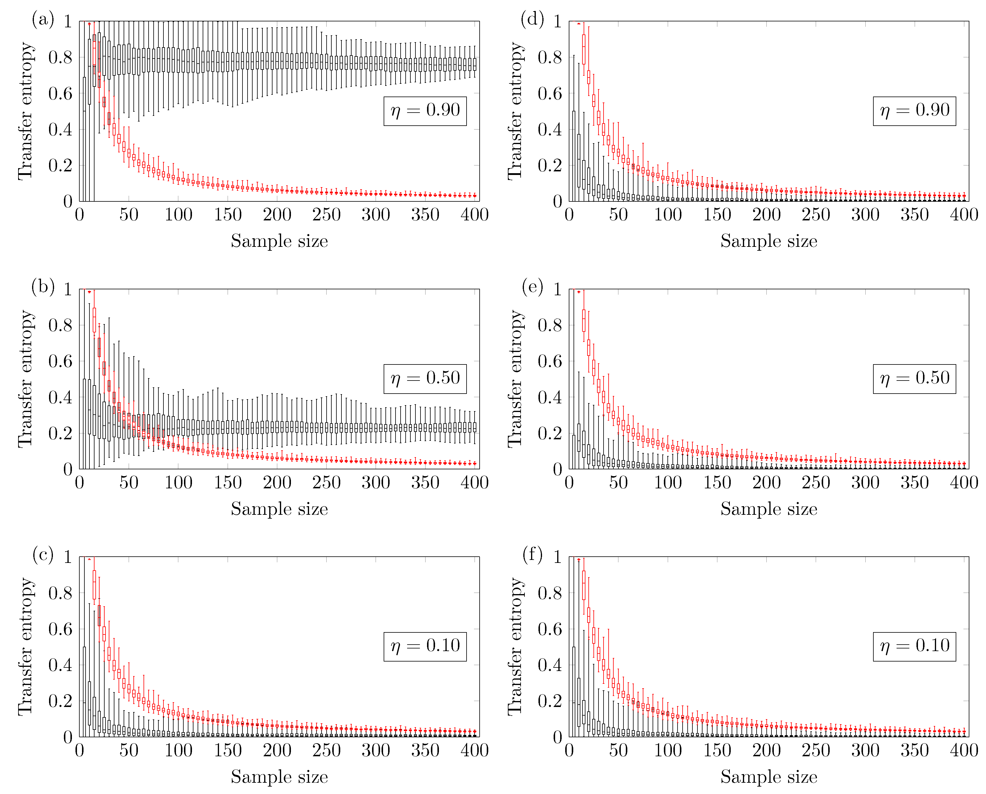
In this section, the minimum sample size required to avoid type II error is pinpointed with a significance level of 4.9%. Figure 2, Figure 3, Figure 4 and Figure 5 show the boxplot regarding the 100 TE values versus the sample size N. The ends of the whiskers represent the minimum and maximum TE values. The TE calculated from the original time series is seen in black, and the threshold (family-wise error rate of 0.0005) is seen in red. The minimum reliable sample size is defined as the smallest N therefore the minimum TE value calculated from the original time series is higher than the maximum TE calculated from the threshold. All statements have been made according to a confidence level of 4.9% (comparison-wise error rate).
4.1. Coupled ARMA[p,q]
Figure 2 shows the results for the two coupled ARMA[1,1] models. The reliable minimum sample size depends on the coupling strength of the model. Figure 2a shows results for coupling strength ; the TE method yields a reliable true positive if one uses . Figure 2b shows results for coupling strength ; the TE method yields a reliable true positive if one uses . Finally, Figure 2c shows results for coupling strength ; no minimum sample size is identified (up to ). This means that there is a higher chance of obtaining false negatives. Figure 2d–f show the TE of versus the sample size. In this case, the methodology presents a negligible chance of type I error, which is the incorrect rejection of a true null hypothesis.
In the particular case of the ARMA[] model, Figure 3 shows that the reliable minimum sample size does not depend significantly on the memory of the autoregressive term. The results refer to the autoregressive window size .
We also investigated the relationship between the reliable minimum sample size and the parameter that regulates the stochasticity. Figure 4a,b show the results for and . One can notice that depends on the ARMA parameter . For , the minimum reliable sample size is , and for , the minimum reliable sample size is . So the higher the parameter is, the larger the value must be to obtain a reliable true positive.
4.2. Couple Logistic Maps
Figure 5 shows that the value here changes more abruptly according to the coupling strength in the nonlinear coupled logistic map if compared with the ARMA model. Figure 5a shows the results for coupling strength of . In this case, one requires sample points for the proper detection of the influence of X on Y. This lower bound is very close to the one identified in the ARMA model with the same coupling strength. Figure 5b shows the results for the coupling strength ; in this case, the number of sample points for a reliable true positive is . For the coupling strength , no minimum sample size is identified (up to ). Figure 5c shows a high probability of obtaining false negatives, so no lower bound is identified. Figure 5d–f show that the TE method presents a negligible chance of type I error.
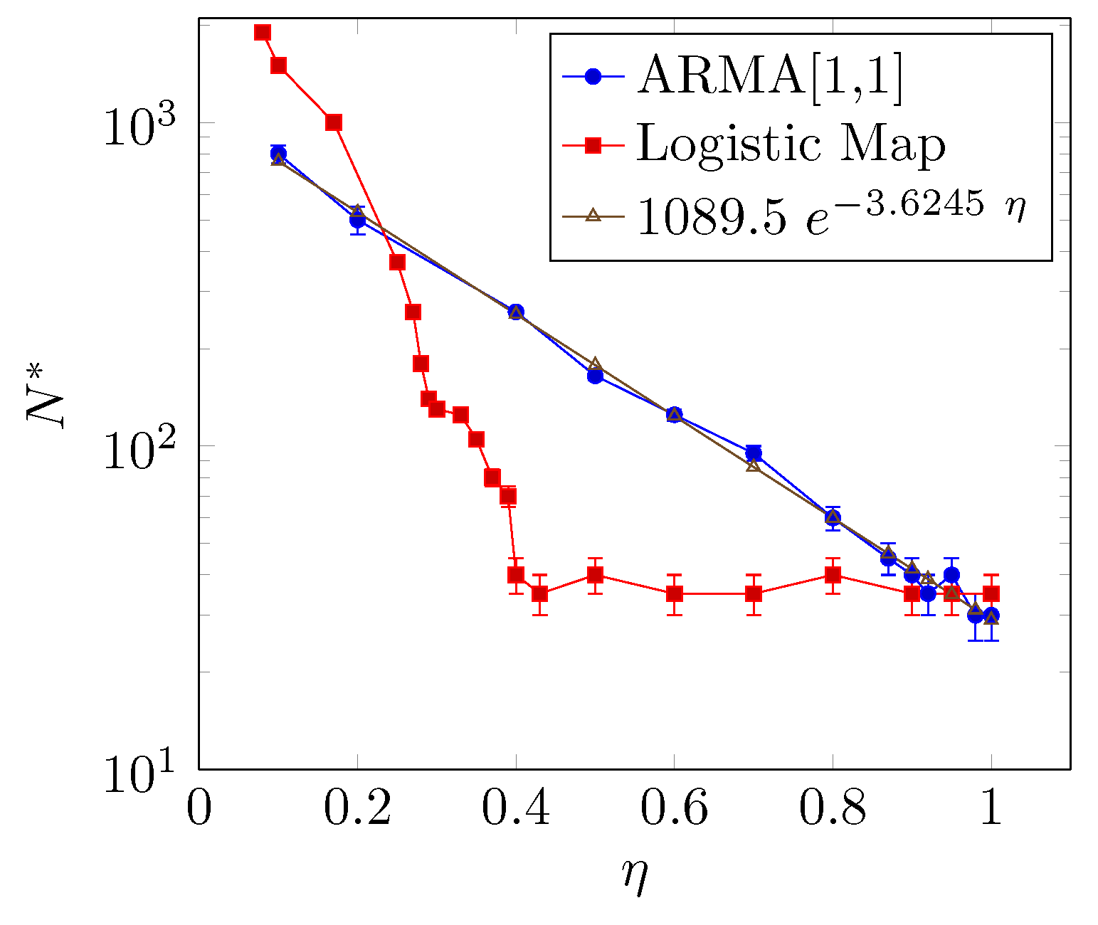
Figure 6 shows the relationship between the reliable minimum sample size and the coupling parameter . The larger the coupling parameter is, the smaller the that is required, but the way decays with is different for the two models. The relationship between and for the ARMA[1,1] model presents an exponential decay, whereas for the coupled logistic map, presents an abrupt decay when and a saturation behavior around for .
The result regarding the coupled logistic map depicted in Figure 6 can be explained as follows: The saturation happens because around , the driven synchronizes its dynamics with the driver. Figure 7a shows the behavior of the system for , i.e., below the synchronization transition. Furthermore, Figure 7b shows the behavior when the system is very close to the synchronized state between the systems with . We stress that this result is important and unexpected because it shows that, even in an almost synchronized state, the underlying methodology can detect interactions correctly.
Moreover, at the high coupling limit, the minimum sample size of the ARMA[1,1] model is , somewhat small if compared with the logistic maps, namely . Despite the fact that this coupling analysis considers only ideal and simplified models, this number can be thought of as the lower bound for the entropy transfer using a significance level of 5% and two ordinal patterns.
4.3. Three Ordinal Pattern
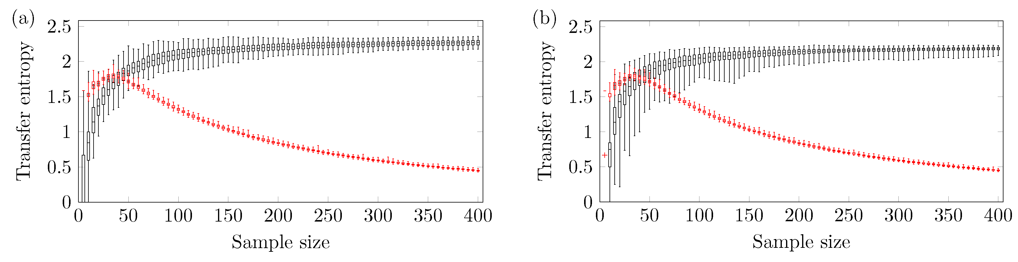
A larger amount of sample points is needed to obtain a reliable outcome using three ordinal patterns. Figure 8 shows the relationship between TE and N using three ordinal patterns and . One can see that the ARMA[1,1] model requires at least sample points, while the logistic model needs at least sample points.
5. Conclusions
In this paper, we have presented a quantitative analysis to find the minimum sample size that produces a reliable true positive outcome using Transfer Entropy. We have tested two paradigmatic models: the linear ARMA model, commonly used in Granger causality approaches; and the well known nonlinear logistic map. The models are constructed to describe two coupled variables X and Y; X influences Y after a lag with coupling strength regulated by the parameter .
The analysis shows that the size of depends on the coupling strength , being the larger and the smaller. This result is expected since the information flow increases with the coupling [5,17], therefore it is reasonable to conclude that the larger the coupling is, the smaller the sample size required to infer causality.
However, the relationship between and depends on the model. For the coupled ARMA model, decreases exponentially as increases whereas, for the coupled logistic map, decays abruptly for followed by a saturation as increases.
Furthermore, at the high coupling limit, the value of approaches sample points. This result establishes the lower bound of the reliable minimum sample size for inference-based causality testing using Transfer Entropy. For this particular case, we use a probability estimation through bipartition of the variable domain. We have shown that the higher the partitioning is, the higher the value is. This methodological procedure can be reproduced for different models, control experimental data and also probability estimation.
Acknowledgments
This research was supported by the São Paulo Research Foundation FAPESP (Grant No. 2015/50122-0, 2014/14229-2 and 2015/07373-2).
Author Contributions
Antônio M. T. Ramos and Elbert E. N. Macau conceived and designed the numerical experiments; Antônio M. T. Ramos performed the experiments; Antônio M. T. Ramos and Elbert E. N. Macau analyzed the data; Antônio M. T. Ramos wrote the paper. Both authors have read and approved the final manuscript.
Conflicts of Interest
The authors declare no conflict of interest.
Appendix A. Probability Estimation
The probability is estimated using the ordinal partitions symbolization [18,19]. The procedure transforms an experimental sample into a sequence of n-tuples called order patterns of size n. Each contains n indexes of the original sample. The indexes are arranged in such a way that their respective values follow an ascending order.
The order patterns are generated by sampling n values with delay , so that the i-sample is defined as . In the context of phase-space reconstruction of dynamical systems, n is also known as the embedding dimension and as the embedding delay [20,21]. In this study, we test and .
The two kinds of models considered here are discrete recurrence relation, so there is no slow response time in the dynamics, therefore no scatter sampling across the time series is necessary. Besides, an embedding delay equal to one is enough for the ordinal patterns to capture the intrinsic features of the model’s dynamics.
Appendix B. Upper Bound of Transfer Entropy
The upper bound of the TE can be obtained through the following consideration: Equations (1) and (2) are devised to make X and Y uncouple when , and conversely, if then Y is entirely described by X. In the latter case, which leads us to . Assuming Y and to be independent, then . This finally leads us to the upper bound of the TE as for equiprobable B partitions in the variable’s domain.
References
- Schreiber, T. Measuring information transfer. Phys. Rev. Lett. 2000, 85, 461–464. [Google Scholar] [CrossRef] [PubMed]
- Balasis, G.; Donner, R.V.; Potirakis, S.M.; Runge, J.; Papadimitriou, C.; Daglis, I.A.; Eftaxias, K.; Kurths, J. Statistical mechanics and information-theoretic perspectives on complexity in the earth system. Entropy 2013, 15, 4844–4888. [Google Scholar] [CrossRef]
- Li, Z.; Li, X. Estimating temporal causal interaction between spike trains with permutation and transfer entropy. PLoS ONE 2013, 8, e70894. [Google Scholar] [CrossRef] [PubMed]
- Runge, J.; Riedl, M.; Müller, A.; Stepan, H.; Kurths, J.; Wessel, N. Quantifying the causal strength of multivariate cardiovascular couplings with momentary information transfer. Physiol. Meas. 2015, 36, 813–825. [Google Scholar] [CrossRef] [PubMed]
- Cafaro, C.; Ali, S.A.; Giffin, A. Thermodynamic aspects of information transfer in complex dynamical systems. Phys. Rev. E 2016, 93, 022114. [Google Scholar] [CrossRef] [PubMed]
- Miller, G.A. Note on the Bias of Information Estimates. In Information Theory in Psychology: Problems and Methods II–B; Free Press: Glencoe, IL, USA, 1955; pp. 95–100. [Google Scholar]
- Green, B.F.; Rogers, M.S. The Moments of Sample Information When the Alternatives Are Equally Likely. In Information Theory in Psychology: Problems and Methods II–B; Free Press: Glencoe, IL, USA, 1955; pp. 101–108. [Google Scholar]
- Sun, J.; Cafaro, C.; Bollt, E.M. Identifying the coupling structure in complex systems through the optimal causation entropy principle. Entropy 2014, 16, 3416–3433. [Google Scholar] [CrossRef]
- Runge, J.; Heitzig, J.; Petoukhov, V.; Kurths, J. Escaping the curse of dimensionality in estimating multivariate transfer entropy. Phys. Rev. Lett. 2012, 108, 258701. [Google Scholar] [CrossRef] [PubMed]
- Wolpert, D.H.; Wolf, D.R. Estimating functions of probability distributions from a finite set of samples. Phys. Rev. E 1995, 52, 6841–6854. [Google Scholar] [CrossRef]
- Holste, D.; Große, I.; Herzel, H. Bayes’ estimators of generalized entropies. J. Phys. A Math. Gen. 1998, 31, 2551–2566. [Google Scholar] [CrossRef]
- Bonachela, J.A.; Hinrichsen, H.; Munoz, M.A. Entropy estimates of small data sets. J. Phys. A Math. Theor. 2008, 41, 202001. [Google Scholar] [CrossRef]
- Barnett, L.; Seth, A.K. Granger causality for state-space models. Phys. Rev. E 2015, 91, 040101. [Google Scholar] [CrossRef] [PubMed]
- Gyllenberg, M.; Söderbacka, G.; Ericsson, S. Does migration stabilize local population dynamics? Analysis of a discrete metapopulation model. Math. Biosci. 1993, 118, 25–49. [Google Scholar] [CrossRef]
- Hastings, A. Complex interactions between dispersal and dynamics: Lessons from coupled logistic equations. Ecology 1993, 74, 1362–1372. [Google Scholar] [CrossRef]
- Roulston, M.S. Estimating the errors on measured entropy and mutual information. Physica D 1999, 125, 285–294. [Google Scholar] [CrossRef]
- Sun, J.; Bollt, E.M. Causation entropy identifies indirect influences, dominance of neighbors and anticipatory couplings. Physica D 2014, 267, 49–57. [Google Scholar] [CrossRef]
- Bandt, C.; Pompe, B. Permutation entropy: A natural complexity measure for time series. Phys. Rev. Lett. 2002, 88, 174102. [Google Scholar] [CrossRef] [PubMed]
- Bandt, C.; Shiha, F. Order patterns in time series. J. Time Ser. Anal. 2007, 28, 646–665. [Google Scholar] [CrossRef]
- Takens, F. Detecting Strange Attractors in Turbulence; Springer: Berlin/Heidelberg, Germany, 1981; pp. 366–381. [Google Scholar]
- Packard, N.H.; Crutchfield, J.P.; Farmer, J.D.; Shaw, R.S. Geometry from a time series. Phys. Rev. Lett. 1980, 45, 712–716. [Google Scholar] [CrossRef]
Figure 1.
Diagrammatic representation of the sampled values used to calculate the Transfer Entropy (TE) between X and Y. The solid black box represents the period of interest and the other two dashed boxes represent the lagged intervals for analysis.
Figure 1.
Diagrammatic representation of the sampled values used to calculate the Transfer Entropy (TE) between X and Y. The solid black box represents the period of interest and the other two dashed boxes represent the lagged intervals for analysis.
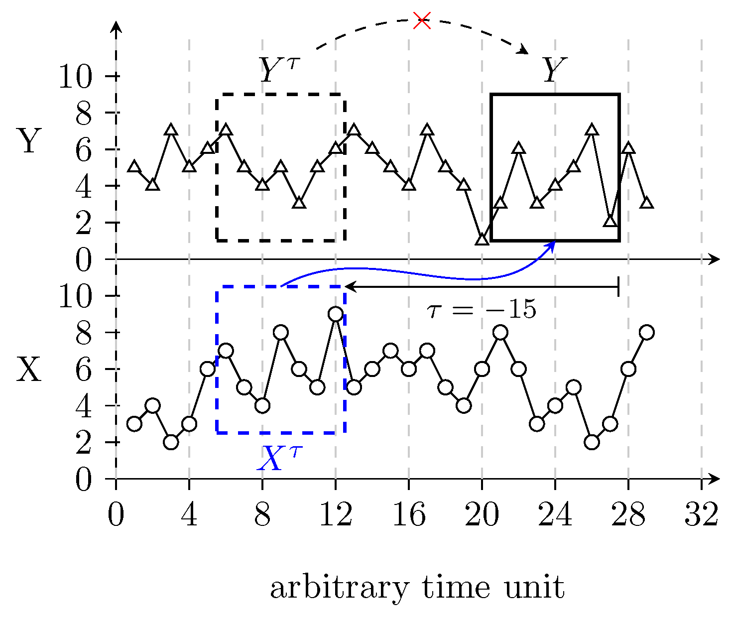
Figure 2.
The black boxplots refer to the time series of the coupled autoregressive-moving-average (ARMA)[1,1] model, and the red boxplots refer to its surrogates. Left: Transfer Entropy of versus the sample size for the following coupling parameter (a) ; (b) ; (c) . Right: Transfer Entropy of versus the sample size for the following coupling parameter (d) ; (e) ; (f) .

Figure 3.
Transfer Entropy of versus the sample size for different autoregressive window sizes (a) , (b) and (c) .
Figure 3.
Transfer Entropy of versus the sample size for different autoregressive window sizes (a) , (b) and (c) .
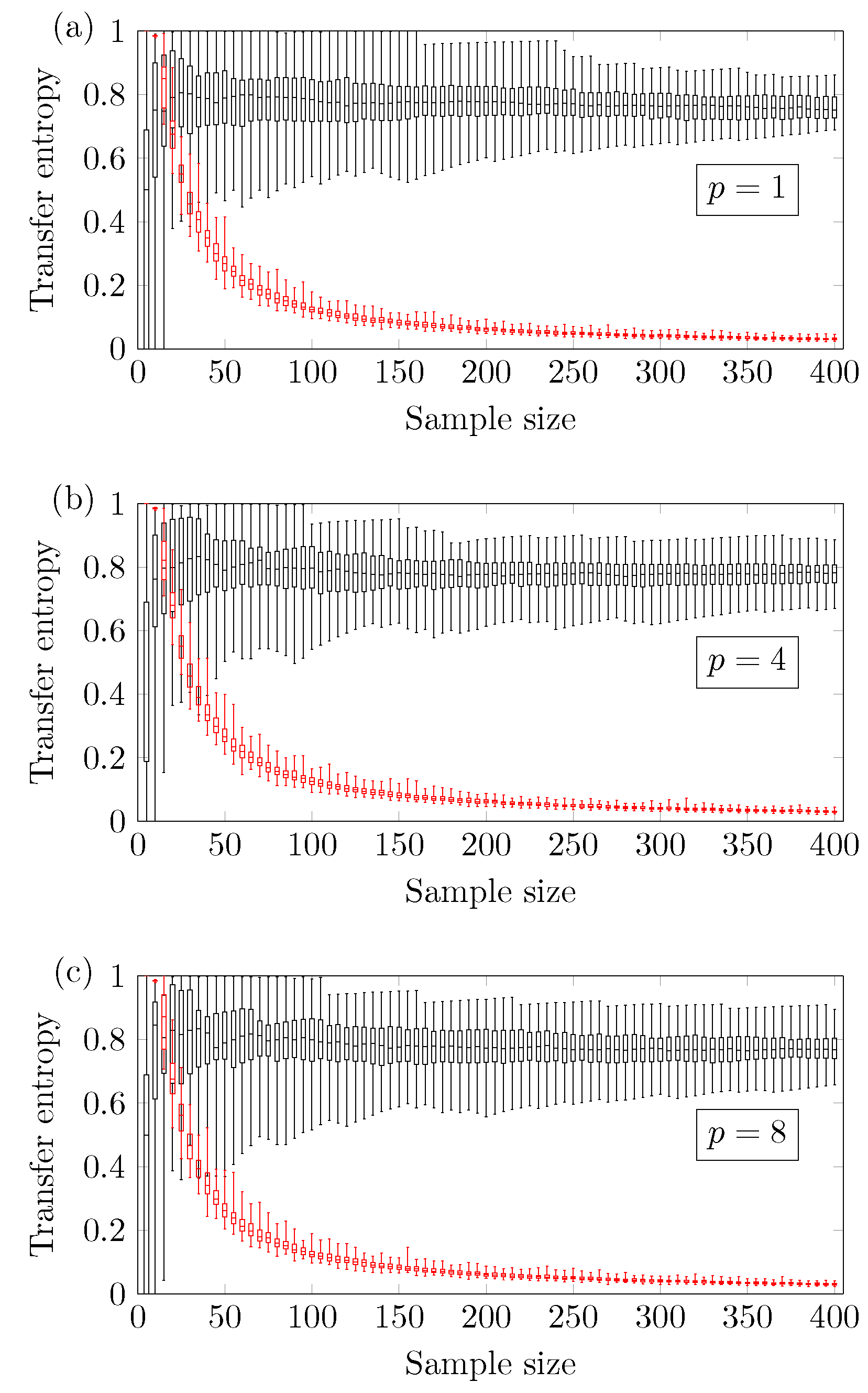
Figure 4.
Transfer Entropy of versus the sample size for different stochastic parameters (a) and (b) .
Figure 4.
Transfer Entropy of versus the sample size for different stochastic parameters (a) and (b) .
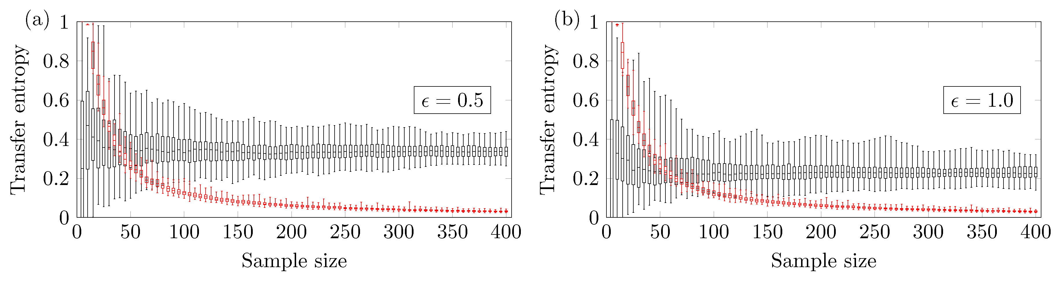
Figure 5.
The black boxplots refer to the time series of the coupled logistic maps, and the red boxplots refer to its surrogates. Left: Transfer Entropy of versus the sample size for the following coupling parameter (a) ; (b) ; (c) . Right: Transfer Entropy of versus the sample size for the following coupling parameter (d) ; (e) ; (f) .
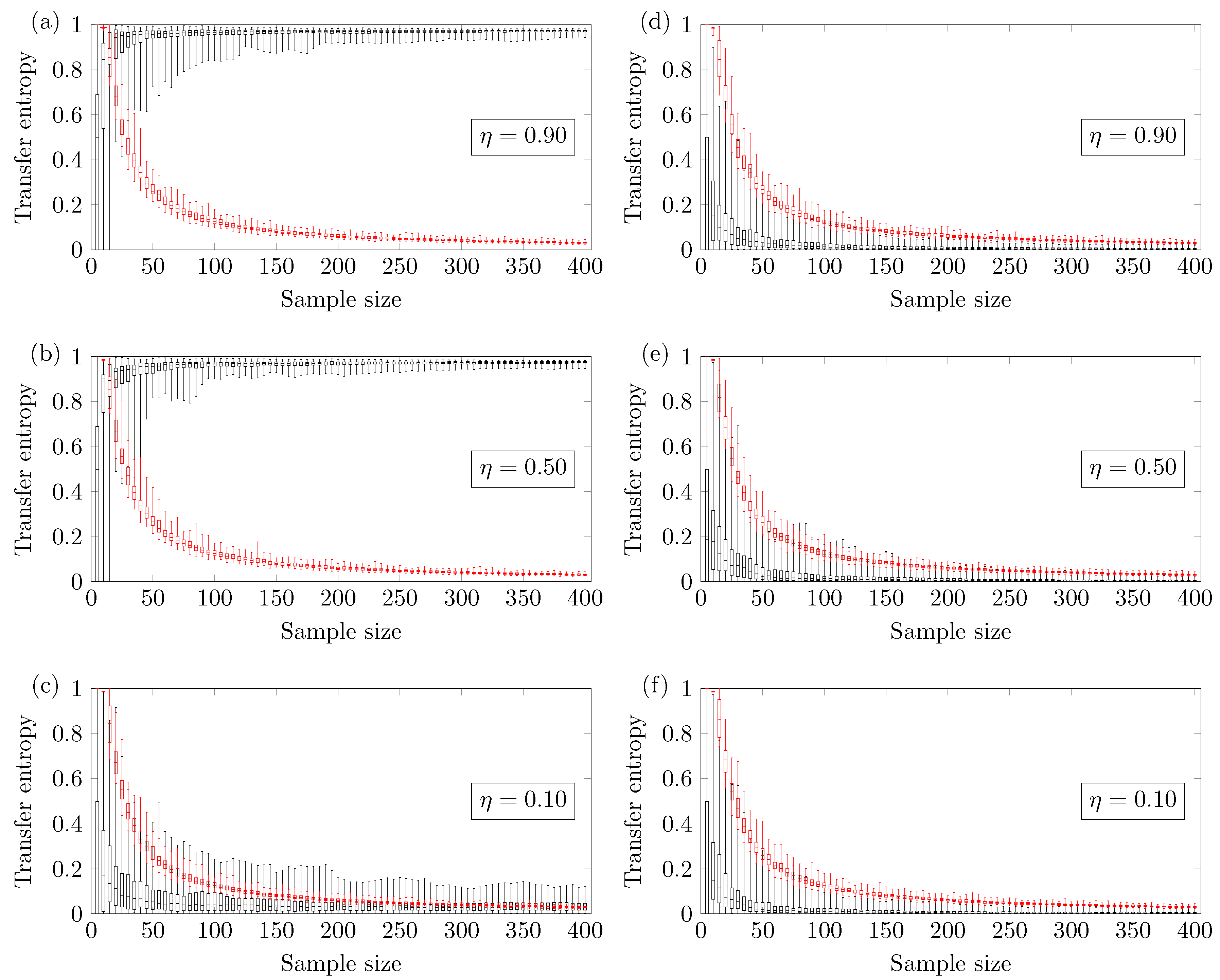
Figure 6.
Reliable minimum sample size versus the coupling parameter , using a binary partition for probability estimation.
Figure 6.
Reliable minimum sample size versus the coupling parameter , using a binary partition for probability estimation.

Figure 7.
Behavior of the coupled logistic maps according to the coupling strength . (a) Shows the behavior when ; and (b) shows the synchronized behavior when .
Figure 7.
Behavior of the coupled logistic maps according to the coupling strength . (a) Shows the behavior when ; and (b) shows the synchronized behavior when .
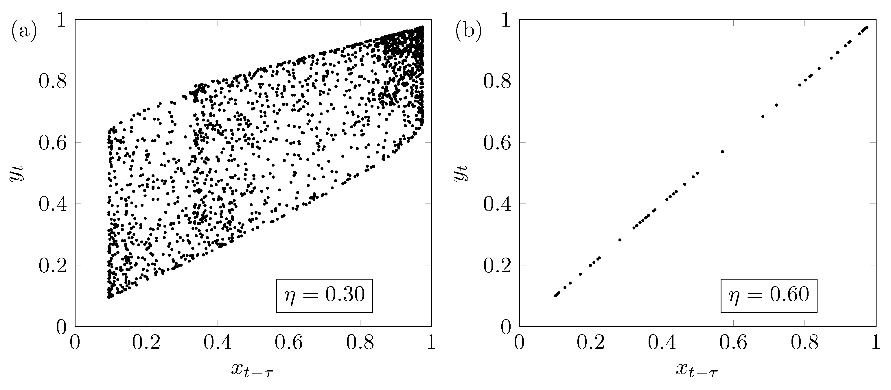
Figure 8.
Transfer Entropy of versus sample size N using three ordinal patterns and coupling parameters . (a) Coupled ARMA[1,1] model; (b) Couple logistic maps.
Figure 8.
Transfer Entropy of versus sample size N using three ordinal patterns and coupling parameters . (a) Coupled ARMA[1,1] model; (b) Couple logistic maps.
© 2017 by the authors. Licensee MDPI, Basel, Switzerland. This article is an open access article distributed under the terms and conditions of the Creative Commons Attribution (CC BY) license (http://creativecommons.org/licenses/by/4.0/).
Share and Cite
MDPI and ACS Style
Ramos, A.M.T.; Macau, E.E.N. Minimum Sample Size for Reliable Causal Inference Using Transfer Entropy. Entropy 2017, 19, 150. https://doi.org/10.3390/e19040150
AMA Style
Ramos AMT, Macau EEN. Minimum Sample Size for Reliable Causal Inference Using Transfer Entropy. Entropy. 2017; 19(4):150. https://doi.org/10.3390/e19040150
Chicago/Turabian StyleRamos, Antônio M. T., and Elbert E. N. Macau. 2017. "Minimum Sample Size for Reliable Causal Inference Using Transfer Entropy" Entropy 19, no. 4: 150. https://doi.org/10.3390/e19040150
Note that from the first issue of 2016, this journal uses article numbers instead of page numbers. See further details here.