1. Introduction
Nowadays, one of the main problems in the oil industry is related with
hydrocarbon reservoir heterogeneity, variability, and anisotropy. All of these properties are very complicated from the point of view of measuring, mathematical modeling, and computer simulation [
1]. From the wild
variability of the data (especially the petrophysical ones) obtained for one rock sample produces unavoidable failure of the extrapolation of results to another seemingly similar one. This problem of not only dramatically poor extrapolability of costly data banks, but also of results averaging, becomes especially dangerous during the scaling of reservoir properties, especially of the “
poroperm” (the relation between the rock porosity and permeability). In the present research, we are looking for the simplified mathematical assumptions to model the rock multiscale geometry with minimum uncertainty. One of the most successful mathematical models is based on exploring the
fractal concepts of similarity and scale invariance, applied to establish the main power law among the pores’ geometrical descriptors, such as the density of the fractures, or other types of pores, per rock volume unit (see, e.g., Oleschko et al. [
2,
3]). The tree-like geometry of percolation networks was always of special interest of Mandelbrot, the father of fractal geometry. In the set of our previous publications [
4,
5,
6] we have discussed the advantages of using the scaling, as well as hierarchical representations of several complex systems. Some simplified models of oil, oil-in-water, and water-in-oil emulsion propagation in capillary networks in random porous media based on their physically real
tree-like geometry were proposed [
4,
5,
6].
Mathematically, such tree-like fractals are represented as ultrametric spaces and there exist well developed theories of fractional (pseudo-)differential equations on such spaces [
7,
8,
9,
10,
11,
12,
13,
14,
15], which were applied in [
4,
5,
6] to represent the dynamics of fluids in these tree-like capillary networks. The class of homogeneous trees with the constant number of vertices,
p > 1, leaving each vertex, the so called
p-adic trees, is especially useful for theoretical modeling as representing a mathematically simple model which, at the same time, represents the basic features of fluids’ propagation through capillary/fractures networks. Notwithstanding,
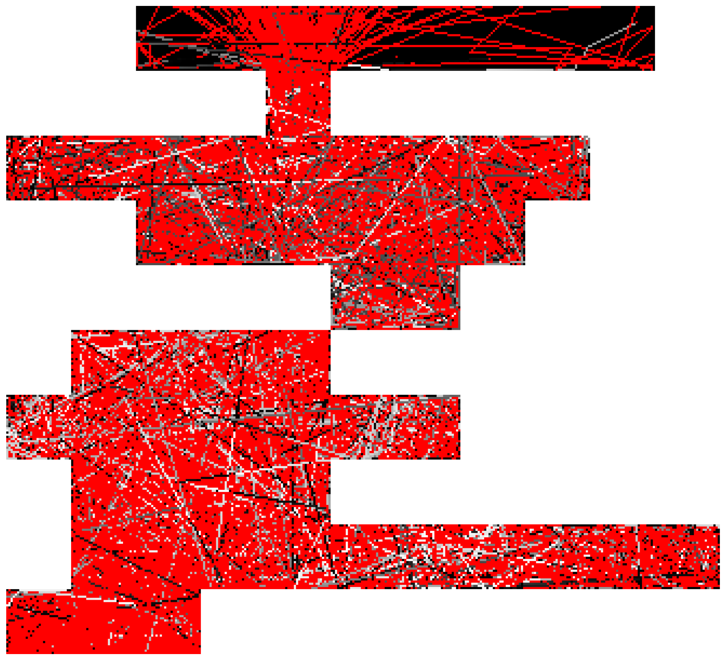
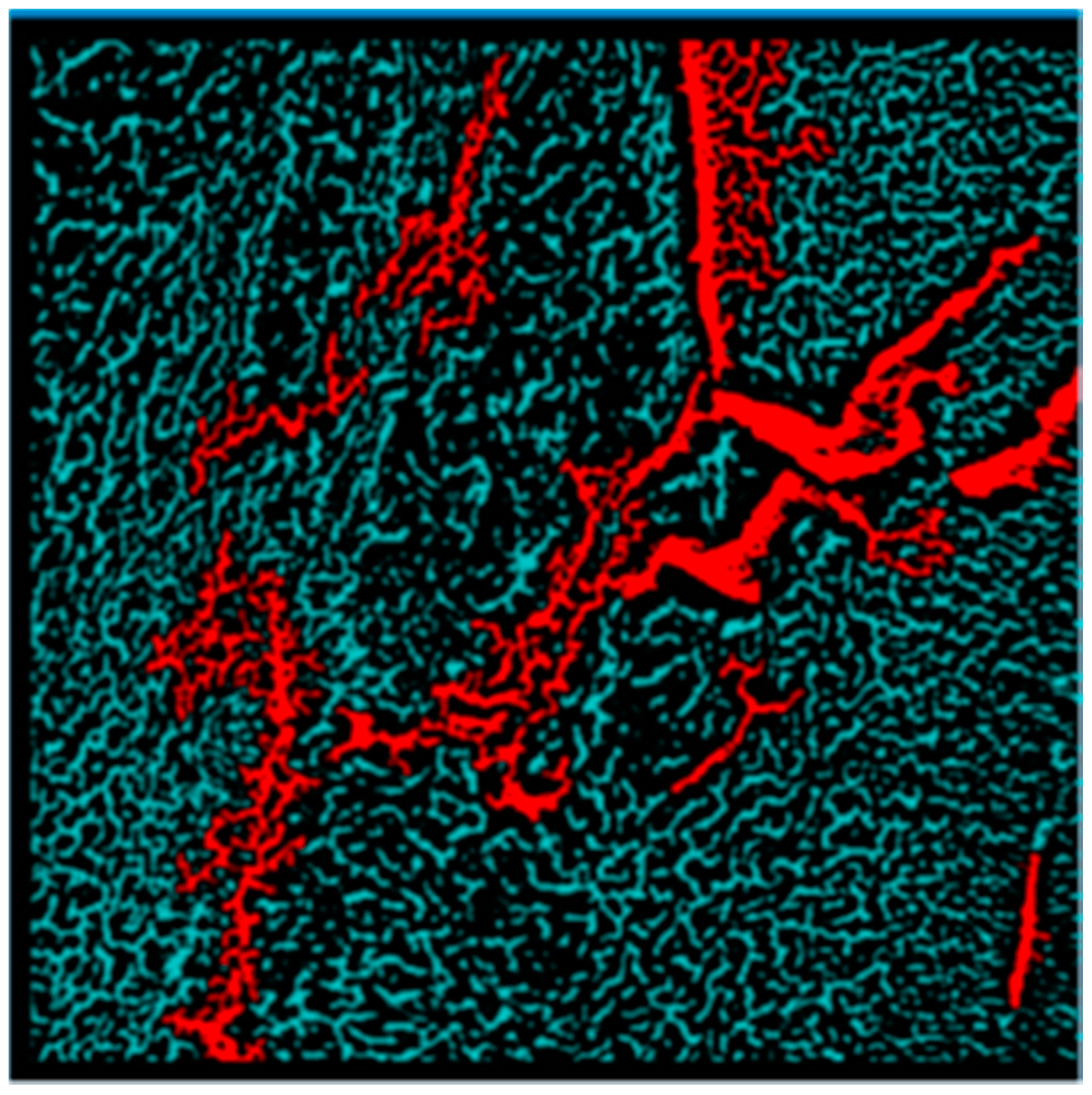
our recent experience has shown that the tree-like geometry is also common for the preferential flow of fluids through fracture patterns on the macroscopic scale (
Figure 1).
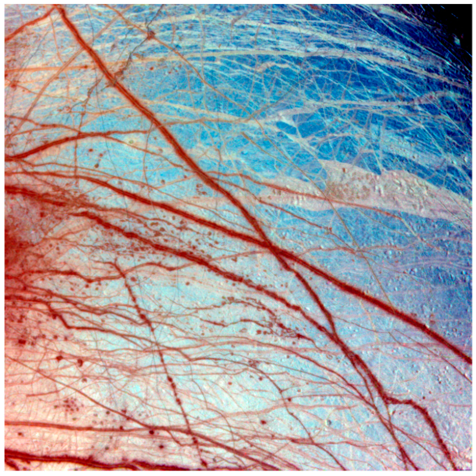
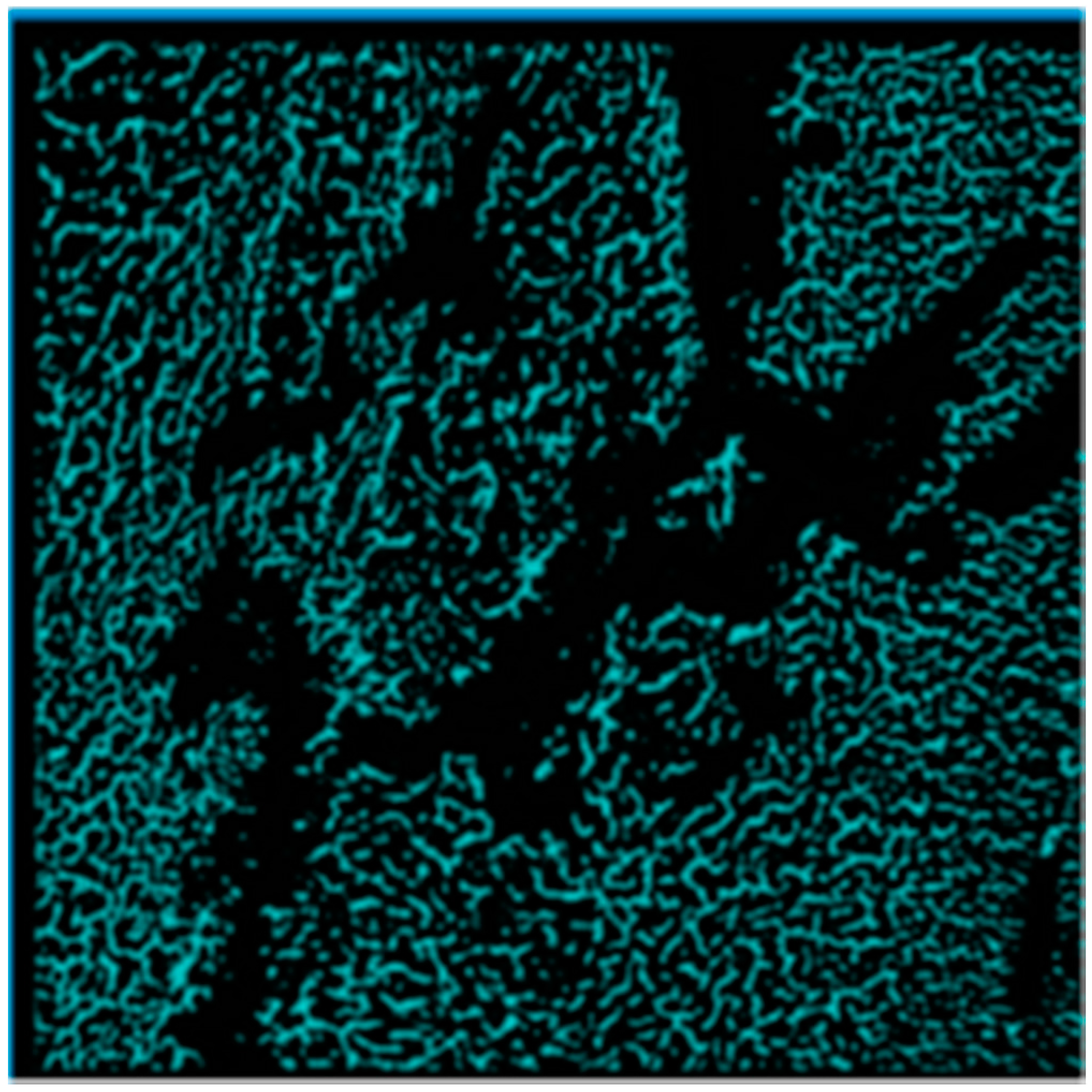
The very similar tree-like geometrical/topological patterns are observed on the mega-scale. The best example came from images obtained by the Voyager spacecraft during the Galileo mission from 1995 to 2003 revealing that the surface of Europa, one of the moons of Jupiter, is crossed by numerous tree-like intersecting ridges and dark bands (called lineae). These features seem to be very similar, at least in appearance, to the Earth fracture system (
Figure 2, courtesy of Dr. P. Geissler). Note, these patterns across Europa´s surface assuggested by numerous scientists [
16], indicate that the thin outer ice shell might be separated from the moon’s silicate interior by a liquid water layer, delayed or prevented from freezing by tidal heating. They were related by Selvans [
17]. with the plate tectonics on ice. By our opinion, and after the recent discovery of geysers on Europa, the water flow network can be related with the tree-like geometry of the surface roughness, observed in
Figure 2.
We point out that, although the ultrametric pseudo-differential equations studied in [
4,
5,
6] describe some distinguishing features of propagation of fluids in capillary networks, they did not explicitly reflect coupling with the physical parameters of such networks. Roughly speaking, they were designed on the basis of abstract reasoning about the natural mathematical form of fluid dynamics on the tree-like configuration space. In this paper we start with dynamical equations matching the tree-like structure to the real physical complex, scaling, and hierarchical systems. The “spatial part” of these equations is given by discrete difference operators (in general nonlinear) representing the hierarchy of interactions at the different levels of a tree. Citing Mandelbrot’s pioneering work, we try to document that the “
randomness is controlled by the geometry of the space” [
21]. We can only add “is controlled by the multiscale geometry of the space and time”.
Similar equations have been used in modeling the hierarchic structure of turbulence flows (see, e.g., [
22,
23,
24,
25,
26,
27,
28]). However, for a moment we can speak only about the mathematical similarity because, in our geo-physical model, the hierarchic structure is given by the geometry of the physical structure, the hierarchic tree-like network of capillaries or fractures (and not by the structure of the process, as in the case of turbulence). The discrete (hierarchic difference operator) structure of the dynamical equations leads to straightforward identification of the physical parameters in their coefficients.
Starting with hierarchic difference equations on capillary trees, we proceed to their “space-continuous” image, where continuity is with respect to the ultrametric topology on a tree. In such an ultrametric continuous limit we obtain the evolutionary equation of which “spatial part” is given by nonlinear
p-adic fractional differential operators. This equation can be treated as the
p-adic analog of the
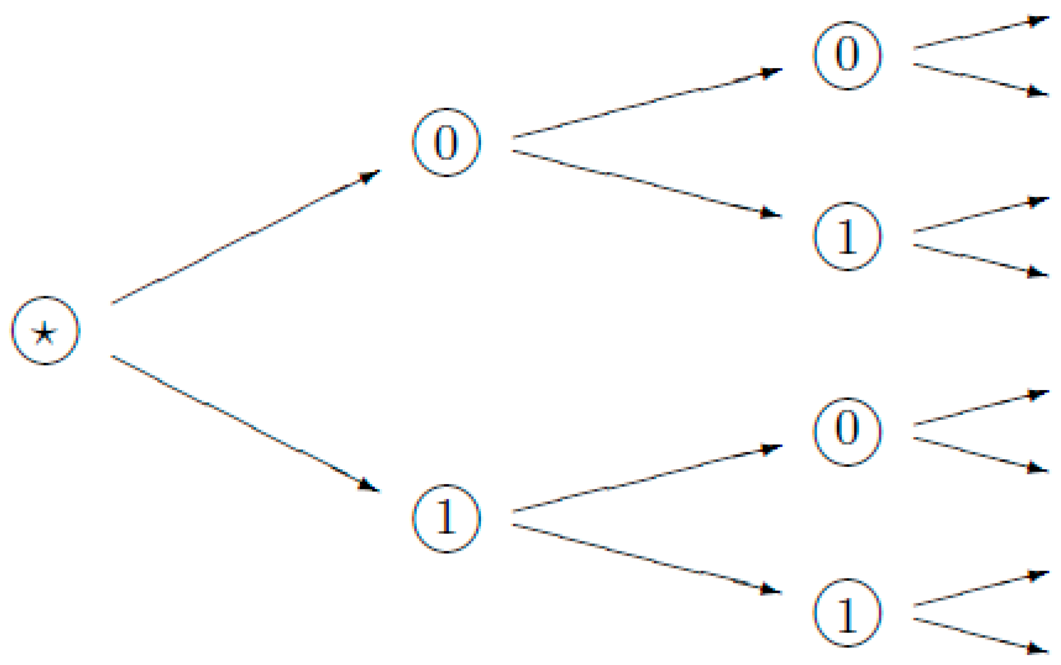
Navier–Stokes equation. In this paper we consider only the simplest binary trees, 2-adic numbers. The reason is very simple: in the very common example of porous media with alternative volumetric expansion and contraction, each fracture is going away from the point of departure in two directions (
Figure 3).
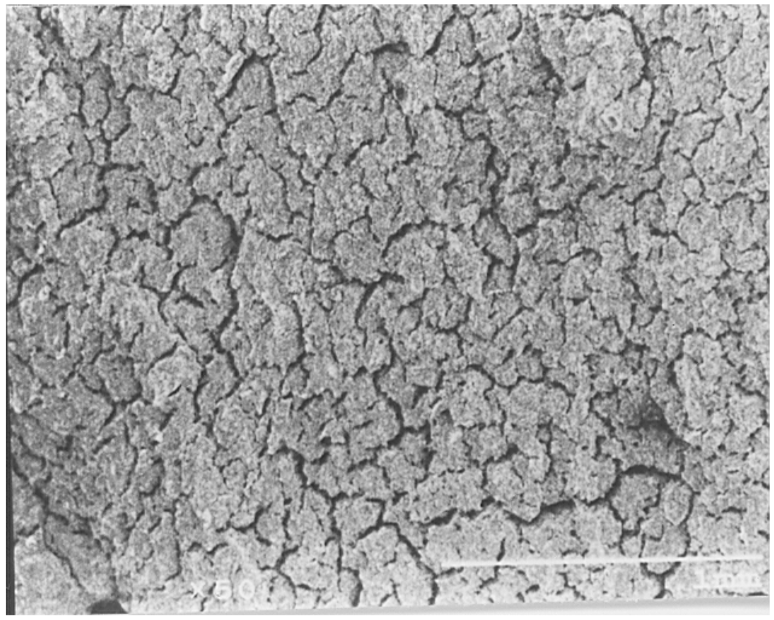
In the case of cracking soil, with high shrink-swell activity associated with the fracture formation (for instance, Vertisol), the fracture density is related by the power law with the number of points of tree-like pore space ramification (
Figure 4).
The general p-adic case, p > 1, can be treated similarly. However, it would be essentially more complicated, technically.
On one hand, our derivation justifies the use of the
p-adic (ultrametric) pseudo-differential equations to model fluid flows in capillary networks in porous media, cf. [
4,
5,
6]. On the other hand, by proceeding from the discrete tree-like dynamics, for which the physical meaning of dynamics’ parameters are well defined, to “continuous” pseudo-differential equations, we also clarify the physical meaning of their parameters. As a purely mathematical consequence of our modeling, we can count stimulation of the interest to development of a general theory of nonlinear ultrametric dynamics.
The paper is structured as follows.
Section 2 is devoted to the brief presentation of the basics about trees and ultrametric spaces.
Section 3 is devoted to the derivation of discrete tree-like dynamical equations describing fluid flows in capillary networks in porous media. In
Section 4 we present essentials of the theory of
p-adic numbers (encoding branches of homogeneous trees) and the corresponding theory of the Fourier transform and pseudo-differential operators (this presentation is really very brief and the reader can find details, e.g., in our paper [
4]). Finally, in
Section 5 we transform the system of discrete tree-like dynamical equations into
p-adic (for the simplest case
p = 2) nonlinear pseudo-differential equations which can be treated as the tree-set analog of the Euclidean space-based system of the Navier–Stokes equations.
Concluding this introductory section we remark that novel applications of ultrametric methods are not restricted to our recent studies in geophysics [
4,
5,
6]. We can also point to a series of studies performed in [
30,
31,
32,
33].
2. Tree-Like Models for Capillary Networks in Porous Media
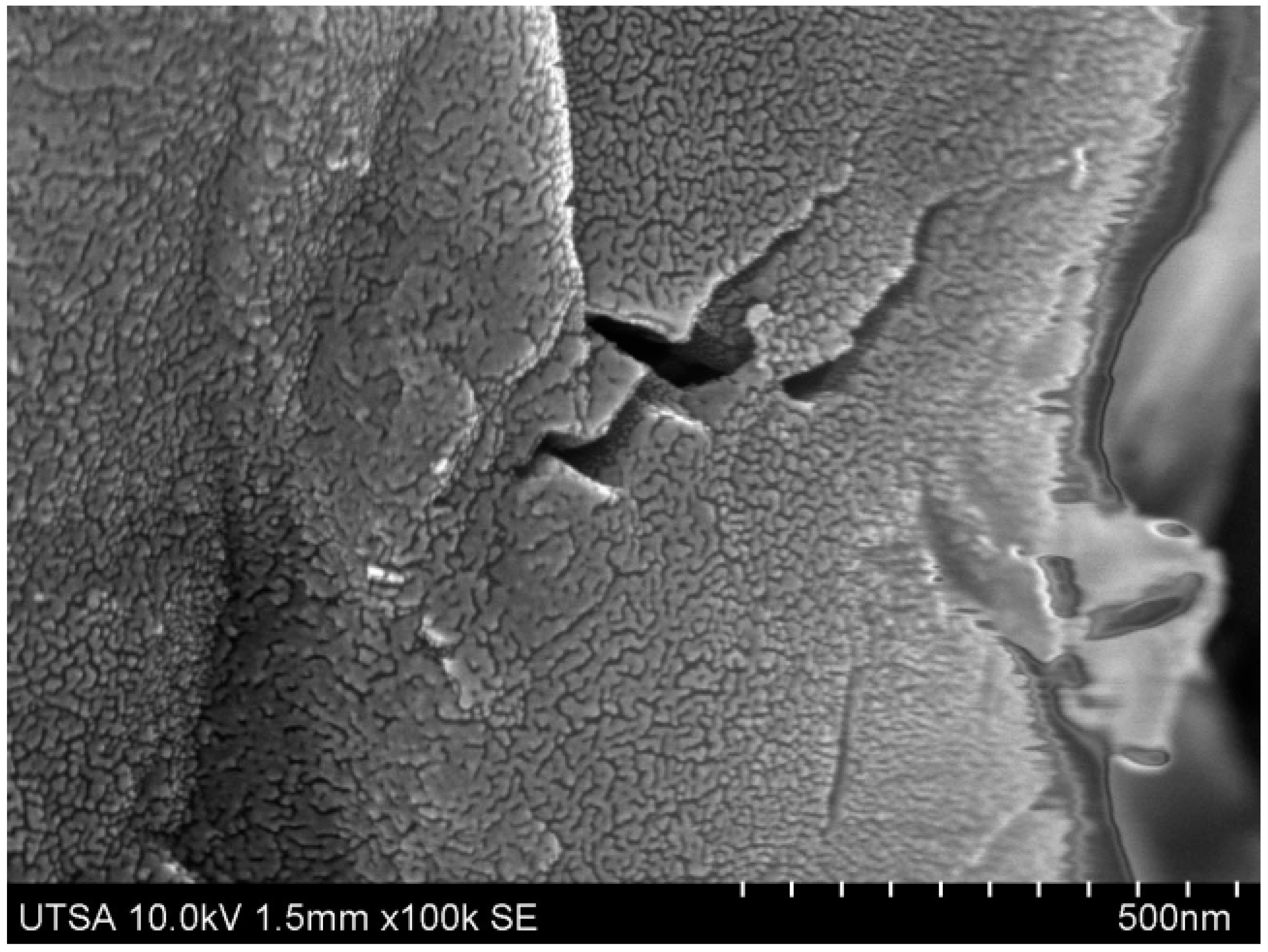
The capillary networks present in rocks have very complex structure (see, e.g.,
Figure 4,
Figure 5 and
Figure 6). Mathematically, they can be represented as graphs of very large variety. In mathematical models, it is very convenient to use approximations preserving some distinguished features of complex spatial objects related to NRFs. The tree-like approximation of the graphs of capillary networks in porous media combines (relative) simplicity with encoding of the
basic fractal features of such networks.
This motivates consideration of the tree-like models, instead of general graphs (although, in real applications, we should proceed with more complex networks which are not reduced to the tree-like objects).
The detailed presentation of the tree-like modeling in geology can be found in paper [
4], with motivations, images from oil industry research, and the corresponding mathematical formalism. Now, we just briefly recall the basics which will be used in the theoretical modeling of fluid flow in capillary networks in
Section 3 and
Section 5.
We start by recalling that a tree is an undirected graph in which any two vertices are connected by exactly one path. We shall work with rooted trees. Such a tree has the special vertex (denoted by the symbol R) which is selected as the root. This is similar to selection of one point in the Euclidean space as the center of the coordinate system. On a rooted tree it is possible to introduce orientations. Each edge can be assigned a direction, either away from or towards R. Such graphs play the important role in graph theory and they are known as directed rooted trees.
Let T be a rooted tree. Let us consider the following (partial) order structure on the set of its vertices. By this order structure, for two vertices, x and y, we set x ≤ y if and only if the path from R to x passes through y. This order structure determines the hierarchic structure on the tree. Consider an arbitrary tree (finite or infinite) T, such that the path in the tree between arbitrary two vertices is finite, and the number of edges incident to each of the vertices is finite. If a vertex I is incident to mI + 1 edges, it has the branching index mI. To each such a tree we shall associate an ultrametric space, so called absolute of the tree. This space is defined in the following way.
The infinitely-continued path starting in the vertex I is a path with the beginning in I, which is not contained in a larger path with the beginning in I.
Let us now fix some vertex R of a tree: its “root”.
The space of infinitely-continued paths in the tree, which begin in the root R is called the absolute of the tree.
This definition does not depend on the choice of the root R. Now we define the metric on the absolute X = X(T) of the tree T. Each x X can be represented as a sequence of vertices starting with the root R, . Take two points x, y X. These two branches have the finite common root-path, with vertices (the kth vertices in branches x and y are not equal). Now we see . One can check that this is the ultrametric on the absolute, i.e., it satisfies not only the usual triangle inequality, but even the strong triangle inequality: ρ(x,y) max[ρ(x,z),ρ(z,y)].
If the tree
T is homogeneous with
mI =
m = const, then ρ(
x,
y)
= 1/
mk. Such homogeneous trees will play an important role in our further modeling,
Section 4 and
Section 5.
3. Tree-Like Analogs of Navier–Stokes Equations
By fixing the special fractal model, namely, the tree-like ultrametric model, we shall derive ultrametric analogs of the basic equations of fluid dynamics, which are based on the commonly used Euclidean space representation of capillary networks. Our equations can be written in the form of nonlinear pseudo-differential equations on ultrametric spaces; see
Section 5 (in fact, we consider the simplest ultrametric tree, the 2-adic tree, in
Figure 7).
In the previous articles [
4,
5,
6] we derived the ultrametric analogs of the probabilistic dynamics based on the balance equations for capillary networks in porous random media. Now we plan to obtain the ultrametric representation of the dynamics of fluid’s velocity (averaged in a capillary). We start with the hierarchic discrete analog of the Navier–Stokes equations in
Section 3.2. These discrete tree-like equations will be transformed into (nonlinear) ultrametric pseudo-differential equations in
Section 5.
One of the problems of theoretical modeling in the ultrametric framework [
4,
5,
6] was establishing the connection between the abstract theory of ultrametric pseudo-differential equations and concrete physical parameters related to fluid flow. Here we shall make a step towards the solution of this problem. Physical parameters incorporated in the discrete tree-like equations are then “lifted” to the corresponding pseudo-differential ultrametric equation.
Our approach leading to a discrete tree-like version of the Navier–Stokes equations is similar to
shell models leading to discrete (in space) chain representations of this equation (see, e.g., [
22,
23,
24,
25,
26,
27]). Instead of linear chains, which are standardly used for the discrete approximation of partial differential equations in the Euclidean spaces, we proceed towards the
tree-structured discrete representations. Thus, we shall take into account the hierarchic tree-like structure of the system of capillaries in porous random media. Here we apply the ideas explored in modeling of the hierarchic structure of turbulent flows of fluid [
26,
27,
28], cf. especially with the model of article [
27]. Although our study is not about turbulence, the mathematics for the simulation of hierarchic flows from [
26,
27,
28] can be applied to our situation, as well as to flows with the internal hierarchy corresponding to a capillary tree.
3.1. Shell Models for the Navier–Stokes Equations
The shell models for the Navier–Stokes equations were elaborated as an attempt to simplify the study of turbulence phenomenon encoded in these equations. As was pointed out, in our research, we are not interested concretely in turbulence. Our interest to the shell models is of the conceptual nature: we treat the shell modeling as a procedure of extraction of the basic features of phenomena described by a complex nonlinear system of partial differential equations.
Consider the standard Navier–Stokes equations:
Here the following variables and parameters are in use: velocity field
u, pressure field
p, viscosity
v, density
d (the latter two are constants), and external force
f. The standard symbolism of the vector-field theory is used (the nabla operator, Laplacian, gradient, vector gradient, divergence):
The main mathematical problem in studies of the Navier–Stokes turbulence is of the following nature [
25]: “Along the line of chaos research, the Navier–Stokes turbulence has come to be considered as a typical and important dynamical phenomenon which is due to a chaotic attractor with, however, a huge dimension estimated to be more than at least some millions by using Kolmogorov scaling argument. Therefore, although it is now widely accepted that the Navier–Stokes turbulence is an example of chaos phenomena, and high-performance computers have become available recently, the computing power is still far from sufficient and properties of the underlying huge dimensional chaotic attractor are not well-understood yet, and especially we do not have an idea of what chaos properties correspond to the well-known robust statistical properties of fluid turbulence as the Kolmogorov scaling and the intermittency”. Thus, one wants to simplify the dynamics and move from the Euclidean continuous space to its discrete model, which is essentially simpler. Our approach is based on the tree-like configuration space and can also be considered as a simplification of the dynamics of fluid propagation in porous media. Instead of the continuous model for such media, we work on the capillary network.
In the standard shell models [
22,
23,
24,
25], instead of the complete Euclidean space representation given by the Cartesian system of coordinates (
x,
y,
z) with the corresponding vector of fluid velocity
,
,
), there are only some special variables that are explored, representing
a shell of the Fourier transform. The new system of equations is
discrete and still nonlinear; the space structure does not present explicitly. One of the basic models is the
Gledzer–Ohkitani–Yamada model [
22,
23,
24,
25]. This model can be considered as a truncation of the Navier–Stokes equations. The physical state of each shell is represented by a single discrete variable
,
n = 0, 1, 2, …. We remark that in the latter model a shell is given by the set of the wave numbers
k:
<
k <
, where
In the shell model representation of the Navier–Stokes equations, only local couplings between nearest (and next to them) neighbor shells are preserved; contribution of others is ignored.
The analogy between the shell representation of the Navier–Stokes equations and our coming tree-like representation is only formal—the split of space into hierarchically-ordered cells corresponds to the split of a tree composed of capillaries into its levels counted from tree’s root. Similarly to the shell model, we exclude the three-dimensional space structure and the new equations are written with respect to specially-discretized and -averaged velocity-field in a capillary network.
The shell models for the Navier–Stokes equations were designed to study turbulence. We have already pointed out that our research is not oriented to turbulence studies. Roughly speaking, we model the capillary size coarse graining for fluid flow in a network of capillaries in porous random media. Such a model matches with the ultraemetric diffusion description. However, the existing hierarchic models of turbulence played the important role of the conceptual background.
3.2. Tree-Like Analogs of the Navier–Stokes Equations: The Case of the Binary Tree
To model the multi-fractal structure of turbulence, in [
26,
27,
28] the shell model of
Gledzer–Ohkitani–Yamada was generalized and the cell-structure was combined with the hierarchic tree-like structure. We now follow the ideas of the work [
27], but just formally, by omitting technicalities. To simplify considerations, we proceed with the 2-adic tree of capillaries (see
Appendix for the general case). It has the root
vertices,
,
,
,
, …,
. We are interested in edges connecting vertices and representing capillaries of the network. They can be labeled in the same way as corresponding vertices, i.e.,
and
there are
edges connecting vertices of the (
n − 1)-th level with vertices of the
n-th level:
or:
In the present model the diameters and lengths of edges are coupled by scaling ½. The 2-adic tree is the simplest ultrametric space; our model can be generalized to the p-adic trees, where p > 1 is a natural number. In such a model lengths and diameters of capillaries are scaled by the factor 1/p. In principle, there are no visible barriers to extend the model to general ultrametric spaces. However, the general case has to be handled more carefully. Ultrametric spaces represent a very general class of trees of capillaries; here the scaling factors for lengths and diameters of capillaries can depend on the concrete vertex.
In contrast to the “Euclidean equations of Navier–Stokes”, our capillary system is constructed of one-dimensional edges. In the present model, motion of fluid, e.g., oil in a capillary is characterized by the averaged (over capillary’s volume) velocity (t). Thus, we are not interested in the velocity at each point of a capillary, but in its average over it.
To write a hierarchic tree-like system of equations for velocity (t), we assume that fluid in the capillary interacts only with fluid in neighboring (from the viewpoint of the tree topology) capillaries, i.e., the dynamics of (t) is determined by functions of (t) and corresponding velocities for the (n − 1)th and (n + 1)th levels. The latter level gives a contribution with (t) and (t). The upper level contributions can be represented in the following way:
Let
j = 2
i − 1 or
j = 2
i, then the (
n − 1)-th level contributes through
(
t). The simplest coupling (similar to the classical Navier–Stokes equations) has the quadratic form. Thus, we obtain the following system of ordinary differential equations representing dynamics in the tree-structured network of capillaries. Here,
denotes the
force acting to the fluid in the
j-th capillary of the
n-th level,
denotes
viscosity, which is assumed to be constant:
Here ; the coefficient A represents the amplitude for the transition of the fluid from the capillary of the previous level to the two “child-capillaries” of the next level; the coefficients B and C represent amplitudes for the transition from the n-th level to the (n + 1)-st level.
This is the simplest hierarchic (nonlinear) system representing, in a “capillary coarse graining” manner, the flow of fluid through the capillary network. It takes into account only the transition from, and to, the nearest levels. A closer analogy with the Navier–Stokes equations can be obtained by taking into account, for each level
n, two successive levels, i.e.,
n − 2,
n − 1 and
n + 1,
n + 2. By omitting the low indices, labeling capillaries of the fixed level of the hierarchy, we can write such generalized systems of dynamical equations for fluid flow in a capillary network as follows:
The system of Equation (3) is a closer analog of the “Euclidean Navier–Stokes equations”. In the tree-like representation the diffusion term of the latter correspond to involvement of not only the closest neighboring levels, but the closest higher and lower levels (tree-like analogy with the second difference scheme, cf. also with the hierarchic shell models, e.g., [
27]). It is easy to represent the system of Equation (3) in the detailed two-index form, as Equations (1) and (2), but it would become too complex and less visualizable.
3.3. Connection with Dynamics on the 2-Adic Space
To couple the discrete tree-like analog of the Navier–Stokes Equations (1), (2), or (3) with theory of
p-adic
pseudo-differential equations (in fact, equations with the
p-adic fractional derivatives, Vladimirov’s operators), we remark that the edge
can be represented by the vertex
or, more precisely, by the pathway starting at the root
and finishing in the latter vertex. Then (see [
3]) each vertex represents the
p-adic ball, in our 2-adic model, the vertex
represents the ball
of the radius
, whose center is determined by the pathway of vertices,
Thus, the capillary coarse-grained velocity
(
t) can be represented as a function of the corresponding ball,
(
t) =
(
t,
) =
). The theory of
p-adic and more general ultrametric pseudo-differential equations was presented in an applications-friendly manner and in significant detail in our recent article [
4]. The mathematical foundations of this theory were set in works [
7,
8,
9,
10,
11,
12,
13,
14,
15] (see also the extended bibliography presented in the monograph [
10]). Our aim is to write the tree-like analog of the Navier–Stokes equations (see Equations (1) and (2)) for the simplest model based on interactions only between three successive levels of the network hierarchy.
We now move to the mathematical representation of the above discussion. Here we have to start with the brief introduction to p-adic numbers (encoding homogeneous tress with p > 1 branches leaving each vertex).
4. P-Adic Numbers, Fractional Differential Operators, Fourier Transform, and Convolution
In this section we briefly present basics of the theory of
p-adic Fourier transform (see [
4] for a non-mathematician-friendly detailed presentation; see also the monograph [
10] for the mathematical details). Consider (see
Section 2) the homogeneous tree with the constant branching index
mI = p, where
p > 1 is the fixed
prime number. The branches of such a tree (which is denoted by
) can be represented by sequences of digits
labeling branches leaving each vertex. Such sequences of digits can be treated as “numbers”, which are formally written as a series with respect to natural powers of
p:
This number representation gives the possibility to introduce on
algebraic operations of addition, subtraction, and multiplication. In algebra such structures are called
rings, i.e.,
is a ring. It is convenient to extend this ring to a
field, i.e., to define the operation of division. The field of
p-adic numbers, denoted by
consists of series of the form:
where
. The
p-adic norm is defined as
, if
x ≠ 0, and
, for
x = 0. It determines the ultrametric on
:
. In the same way, as for real numbers, we can introduce the fractional part
for
p-adic numbers.
Let us remember that there exists a Haar mesure
μp on
. Now we define the
Fourier transform of a function
in the following way:
where
is the
additive character on In real analysis the Fourier transform can be used for the integral representation of usual differential operators,
,
n = 1, 2, …. Generalization of this representation to fractional degrees leads to fractional differential operators
which play an important role in many applications, including reaction-diffusion equations used in geology. This is the very special case of pseudo-differential operators. The
Vladimirov operators of
p-adic fractional differentiation (for α > 0) is defined as:
On
p-adic trees these are no straightforward analogs of the usual differential operators (even for α = 1). However, these are the straightforward generalizations of
pseudo-differential operators which are defined with the aid of the Fourier transform. We list a few basic properties of the
p-adic Fourier transform and Vladimirov operators:
where the
convolution of two functions,
u and
v, is defined by the usual integral formula:
Of course, the existence of the convolution integral is a separate mathematical problem. However, in this paper, we shall proceed formally. In particular, we have:
5. From the Discrete Hierarchical Dynamics to P-Adic Pseudo-Differential Equations
In
Section 3 we presented the system of dynamical equations (see Equations (1) and (2)), reflecting the tree structure of a capillary network in porous media. This system accounted for interactions between fluid volumes in neighboring capillaries, where neighboring is with respect to the ultrametric topology of a tree (in our concrete model, the 2-adic tree). As in standard shell models, Equations (1) and (2) can be treated as the discretized (and hierarchically ordered) versions of the dynamical equations of the Fourier amplitude,
. Here the
k-variable is the dual variable to the “spatial variable”
x varying on the 2-adic tree of capillaries. The linear term,
, corresponds to the 2-adic diffusion process driven by the second order (pseudo-)differential operator
. The quadratic (with respect to the velocity) term,
represents a discretized version of the Fourier transform of the product of a function and its “derivative”, namely, of the term
u Du. We also remark that in Equations (1) and (2) the Fourier transform of
Du produces multiplication by the discretization
of the
k-variable. Thus, in the continuous version of the system Equations (1) and (2) of discrete equations has the form:
Now by using the inverse Fourier transform, we obtain the
p-adic pseudo-differential equation:
where
This equation can be treated as the
p-adic analog of the Navier–Stokes equation.
This is a nonlinear
p-adic pseudo-differential equation. The mathematical theory of such equations has not yet been developed (see [
11] for one special example). We hope that the presented derivation of Equation (6) from the system of hierarchic equations for fluid flow in a capillary network in porous media will stimulate purely mathematical research to build such a theory.

