
Multi-Scale Permutation Entropy Based on Improved LMD and HMM for Rolling Bearing Diagnosis


1
Joint Research Lab of Intelligent Perception and Control, School of Electronic and Electrical Engineering, Shanghai University of Engineering Science, 333 Long Teng Road, Shanghai 201620, China
2
Department of Industrial Engineering, University of Salerno, Via Giovanni Paolo II 132, 84084 Fisciano, Italy
3
School of Information Science and Technology, East China Normal University, Shanghai 200241, China
4
Ocean College, Zhejiang University, Hangzhou 316021, China
*
Author to whom correspondence should be addressed.
Entropy 2017, 19(4), 176; https://doi.org/10.3390/e19040176
Submission received: 8 January 2017
/
Revised: 3 March 2017
/
Accepted: 14 April 2017
/
Published: 19 April 2017
(This article belongs to the Special Issue Wavelets, Fractals and Information Theory II)
Abstract
:Based on the combination of improved Local Mean Decomposition (LMD), Multi-scale Permutation Entropy (MPE) and Hidden Markov Model (HMM), the fault types of bearings are diagnosed. Improved LMD is proposed based on the self-similarity of roller bearing vibration signal by extending the right and left side of the original signal to suppress its edge effect. First, the vibration signals of the rolling bearing are decomposed into several product function (PF) components by improved LMD respectively. Then, the phase space reconstruction of the PF1 is carried out by using the mutual information (MI) method and the false nearest neighbor (FNN) method to calculate the delay time and the embedding dimension, and then the scale is set to obtain the MPE of PF1. After that, the MPE features of rolling bearings are extracted. Finally, the features of MPE are used as HMM training and diagnosis. The experimental results show that the proposed method can effectively identify the different faults of the rolling bearing.
1. Introduction
Rolling bearings are the most important parts of rotating machinery, which are easily damaged by load, friction and damping in the course of operation [1]. Therefore, the feature extraction and pattern recognition of bearings diagnosis are very important. The time-frequency analysis method has been widely used in faults diagnosis, because it can provide the information in the time and frequency domain [2]. Moreover, there are many methods of artificial intelligence detection, such as statistical processing to sense [3], stray magnetic flux measurement [4], and neural networks such as support vector machine (SVM) [2].
When the wavelet basis function of the wavelet transform (WT) [5] is scheduled to be different, the decomposition of the time series will have great influence. When the wavelet base is selected, WT has no self-adaptability at different scales [2,6].
Empirical mode decomposition (EMD) [6] can involve the complex multi-component signal adaptive decomposition of the sum of several intrinsic mode function (IMF) components. Further, the Hilbert transform of each IMF component is used to obtain the instantaneous frequency [7,8] and instantaneous amplitude. The aim of this is to obtain the original signal integrity of the time-frequency distribution [9], but there are still some problems, such as: over-envelope, under-envelope [10], modal aliasing and endpoint effect in the EMD method.
The Local Mean Decomposition (LMD) [2] method realizes signal decomposition and demodulation by constructing the local average and envelope estimation functions, which effectively solves the problem of the over-envelope, under-envelope and modal aliasing in the EMD method [6]. Compared with WT and EMD, LMD has the nature of self-adaptive feature and the LMD endpoint effect involves a certain degree of inhibition, while solving the problem of under-envelope and over-envelope.
Researchers have found that the endpoint effect processing has been improved by LMD [11,12,13], but the impact of the endpoint effect is still very obvious, and it cannot be proved that extreme ones use the left or the right points, so we can not explain how the envelop curve fitting function of the extreme value may be reasonable [5]. Researchers have found that the LMD edge effects can be solved by the extreme point extension and the mirror extension [9]. The boundary waveform matching prediction method contains the Auto-Regressive and ARMA prediction [7]. Both sides of the waveform are just extended by these methods, but these methods do not take into account the inner rules or characteristics of signals. The new improved LMD takes inner discipline into account, the results of experiments show that the new method is more flexible than the existing method.
After the improved LMD decomposition, we have to solve a major important aspect, namely, how to extract the fault information from the obtained PF components. Many studies have been carried out to solve the problem. In recent years, mechanical equipment fault diagnosis is used more than non-linear analysis methods such as sample entropy and approximate entropy [14,15,16]. Permutation Entropy (PE) [15,16,17] is a new non-linear quantitative description method, which can be a natural system of irregularities and a non-linear system in the quantitative numerical method presented, and has the advantages of simple calculation and strong anti-noise ability. However, similar to the traditional single-scale nonlinear parameters, PE is still in a single scale to describe the irregularity of time series.
Aziz et al. [18] proposed the concept of MPE. MPE can be used to measure the complexity of time series under different scales, and MPE is more robust than other methods [18]. However, mechanical system signal randomness and noise interference are poor. The MPE method is used for signal processing, and the detection result is unsatisfactory. Therefore, MPE is used in combination with LMD, forming a new high-performance algorithm, which can effectively enhance the effectiveness of MPE in signal feature extraction.
In this paper, the rolling bearing vibration signals were decomposed into several PF components by improved LMD. Then, the phase space reconstruction of the PF1 is carried out by using the mutual information (MI) and the false nearest neighbor (FNN) to calculate the delay time and the embedding dimension, and then the scale is set to obtain the MPE of PF1. After that, the feature vectors are extracted as the HMM and back-propagation (BP) neural network input, and then the training diagnosis and fault diagnosis are compared.
2. Improved LMD Method and Phase Space Reconstruction of MPE
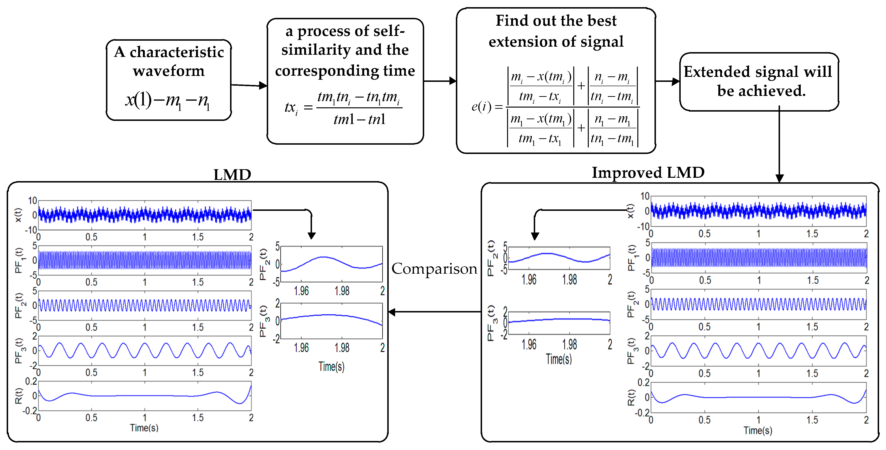
The process of improved LMD is summarized in four sub-processes, first we set up three points to invest a triangular waveform, and then we list all start points (it will takes some time to search the characteristic waveform), finally we get the best integration interval. After that we will study the shape error parameters to get the best extension of signal. Finally, we extend the right end through the above method, and the extended signal will be better.
Figure 1 will show that the edge effect has become better, the end of the time-frequency representation changes significantly. Therefore, the experiment shows that the improved LMD has greatly improved the reduction of the border.
In Figure 2, the vibration signals of the rolling bearing are decomposed into several PF components by the improved LMD respectively. Then, the phase space reconstruction of the PF1 is carried out by using the MI and the FNN to calculate the delay time and embedding dimension, and then we can set the scale to obtain the MPE of PF1.
In Figure 3, MI [17,18,19,20] determines the optimal delay time. represents a group of signals, the probability density function of the point is , the signal is mapped to the probability .
The two groups of signals are measured probability density . In the formula: and respectively correspond to and of the entropy in the specified system and measure the average amount of information; is a joint information entropy.
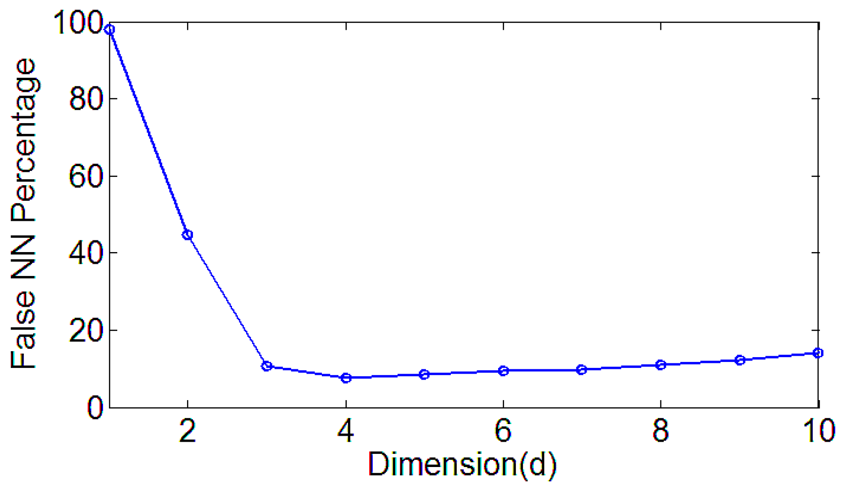
In Figure 4, FNN [21,22,23,24] is used to calculate the minimum embedding dimension effective method. Time series constructs a dimension space state space vector . Using to represent the nearest neighbor, the distance between them can be calculated by the formula.
When the embedded dimension changes from m to , a new coordinate is added to each component of the vector . At this time, the distance between and is the relative increment of the distance, so they are false neighbors.
In the calculation of the project , it is found that the false neighboring points can be easily identified. At the time , we call the nearest neighbors, by computing each nearest neighbor of the trajectory.
In order to make the MPE have better fault recognition effect, it is necessary to use the MI and the FNN to optimize the delay time and the embedding dimension when calculating the MPE in Figure 2. The MPE is calculated based on the optimized parameters.
3. Diagnosis Flow Based on HMM
- (1)
- The characteristic index of bearing failure degree is extracted from the fault signal of the needle roller bearing with different degrees of damage, and the feature index is normalized and quantized [24]. When the HMM is established, the sequence of observations should be a finite discrete value, and the discretized value can be used as the model training eigenvalue after quantization.
- (2)
- Diagnosis Flow Based on HMM [25] in Figure 5. The Baum–Welch algorithm [26,27] is used to train, adjust and optimize the parameters of the observation sequence, so that the observed sequence of probability values in the observed sequence is similar to the observed value sequence. We calculate the maximum, HMM state identification, different fault levels of the state to establish the corresponding HMM, the unknown fault state data and in turn enter the various models, calculate and compare the likelihood. The output probability of the largest model is the unknown signal fault type. It is estimated that the most probable path through the sequence is observed by the Baum–Welch algorithm.
4. Experimental Data Analysis
In Figure 6, in order to validate the proposed method, the experimental data of different rolling bearings are analyzed. The experimental data are analyzed from the Case Western Reserve University. The bearing of the drive shaft end is the 6205-2RS SKF deep groove ball bearings, and the loaded 2.33 kW motor. The pitch diameter of the ball group is 40 mm and the contact angle is 0, the power of motor is 1.47 kW. Sampling frequency is 12 kHz and the relevant drive motor speed is 1750 rpm with 2 Hp load, the number of sampling points n = 2048. The collected signals can be divided into four fault types including Normal, IRF, ORF, and BF. Each condition has 16 samples and a total of 64 samples.
The normal state of the bearing, inner ring fault, outer ring fault and rolling body fault are tested. Due to limited space, only the improved LMD decomposition of the inner ring fault is listed in Figure 7. We can find that improved LMD decomposition is performed for each group of time domain signal, which sets the amount of change. The multi-component AM-FM signal is decomposed into a single component AM-FM signal, the decomposition of the PF component and the signal correspond to the corresponding components, which reflect the various components of the signal in the presence of different characteristics of components. Each PF component has a physical meaning, reflecting the original signal of the real information, so we get a series of PF components.
We can obtain the signal after improved LMD decomposition, which can effectively remove noise, and extract important signals. PF1 is more than 80% of the original information. PF1 can effectively reflect the original signal of the complete information characteristics. Therefore, we use the PF1 to calculate the MPE. Not only can we improve the computational efficiency, we can also reflect the original information characteristics.
According to the calculation steps of the MPE, the phase space is reconstructed. Delay time and embedding dimension are two main parameters influencing the MPE algorithm. It is determined that these two parameters have certain principal randomness. Therefore, we need algorithms for phase space reconstruction. Phase space reconstruction methods mainly have the MI and the FNN to determine two parameters independently and the (C-C) joint algorithm. We found that MPE obtained by independent parameters has a better mutation detection effect. So the important PF1 component can be selected by the MI and the FNN to calculate the delay time and the embedding dimension. After that we reconstruct the phase space.
We can set the MI parameter, Max_tau = 100, the program default maximum delay Part = 128 and the program default box size. The delay time is calculated by the MI, as shown in Figure 3. On the basis of determining the delay time, the false nearest neighbor method is adopted to optimize the embedding dimension, where the maximum embedding dimension is set to 12, the criterion 1 is set to 20, criterion 2 is set to 2, false neighbor rate with the embedding dimension of the curve as shown in Figure 4. When the embedding dimension is 4, the FNN rate is no longer reduced with the increase of the embedding dimension, so the embedding dimension is set to m = 4. Using the same principle, we can reconstruct the four faults of the rolling bearing with phase space, and calculate the delay time and the embedding dimension. Due to the limited space, we only list part of the delay time and embedding dimension, and Table 1 reflects the partial delay time and the embedding dimension.
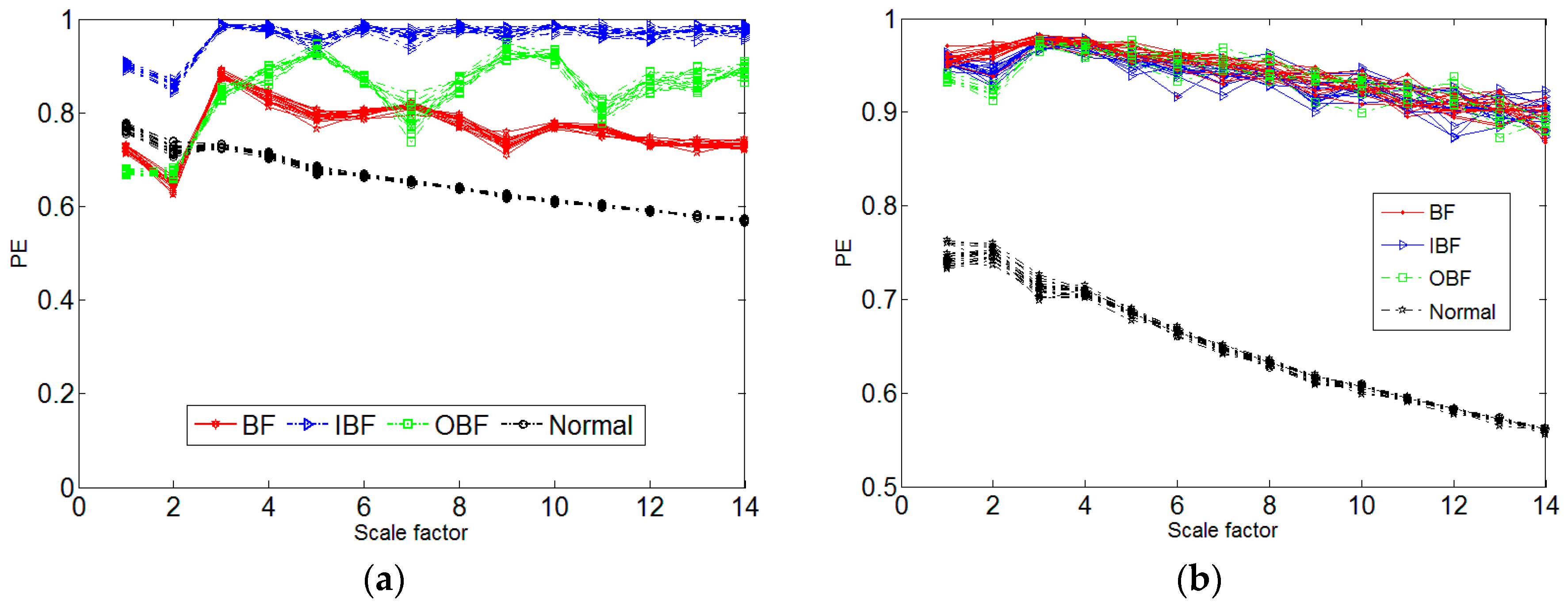
After the phase space reconstruction, the delay time and embedding dimension are used to compute the MPE. We define the scale factor S and calculate the MPE, select the PF1 component of the data length N = 2048, the scale S = 14. Therefore, we can calculate the MPE. In Figure 8, the MPE of PF2 is compared with MPE of PF1. We can see that PF1 is better than PF2, so we choose PF1. We can see that the rolling body faults and the inner ring faults are well distinguished, but the outer ring faults cannot be very good. Therefore, there is a need to identify the model, it is HMM. After the MPE is calculated, the feature vectors are grouped into an Eigenvectors group for the input of HMM and the BP neural network, and trained and predicted for different faults.
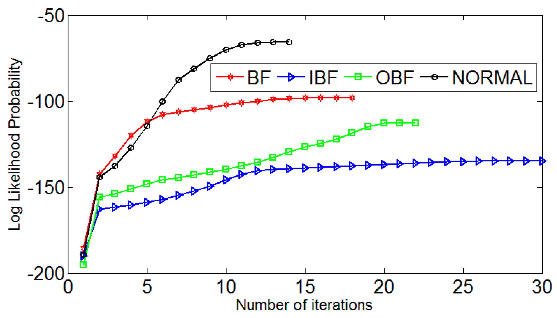
The training curve is shown in Figure 9. HMM modeling and training, rolling body fault, inner ring fault, outer ring fault, and the normal bearing represent four kinds of hidden state, recorded as λ1, λ2, λ3, λ4, respectively. The observation sequence of the model is the six multi-scale permutation entropy feature sequences extracted above. In addition, the state transition probability matrix Bλ shows the initial probability. The distribution vector πλ is generated by the Rand random function, and the training process is normalized. The Markov chain in HMM is described by π and A. Different π and A determine its shape. The features of Markov chain are as follows: it must start from the initial state, along the state sequence, the direction of transfer increases, and then it stops in the final state. The model better describes the signal in a continuous manner over time. The level of bearing failure establishes HMM. Because there are four kinds of fault state, we choose four HMM states, and the model parameter N is chosen. Each state takes 11 groups as the training sample is used to generate HMM under four states, the remaining sets of feature vectors are used as test samples. The training algorithm used is the Baum–Welcm algorithm. We set the number of iterations to 100 and the convergence error to 0.001. In the model of training, the maximum likelihood estimation value increases s the iteration number increases. The training ends when the convergence error condition is satisfied.
In order to prevent the model from getting into an infinite loop or training model failure, the training algorithm uses the Lloyd algorithm to scalar quantify the entropy sequence, and the scalar quantization sequence is input into the HMM. The training algorithm uses the Baum–Welch algorithm. As the number of iterations increases, the maximum log-likelihood estimate increases until convergence is reached. After training, four hidden HMM recognition models can be obtained. Figure 9 shows the HMM training curves for four states. It can be seen that all the states reach convergence at 20 iterations and converge quickly. After the training HMM models, the remaining 20 sets of entropy eigenvectors, fives states of each state, are taken as test samples. Before the test, the sample entropy sequence is scaled by Lloyd algorithm, and the scaled quantized sample entropy sequences are inputted to each state.
After the completion of HMM training in four states, a state classifier is built. The Eigenvalue sequences of the remaining four states is calculated by the Forward–Backward algorithm at λ1, λ2, λ3, and λ4 Model. The log-likelihood of this sequence is generated. Log likelihood probability reflects the degree of similarity between feature vector and HMM, the larger the value, the closer the observed feature sequence is to the HMM of the state. The feature sequence corresponds to the output log likelihood probability value. The maximum model corresponds to the fault state. In the HMM model, each model outputs a log likelihood estimate. The log likelihood estimate represents the degree of similarity between the feature vector and each HMM. The larger the log likelihood estimate, the closer the feature vector in this state HMM model, the recognition algorithm is the Baum–Welch Algorithm.
The log likelihood ratio obtained from the training model inputted to this state is larger than the log likelihood probability value obtained from the other state inputs. In Table 2 it can be seen that the higher the failure degree of the same fault type, the higher the log likelihood estimate is, and the output of natural logarithm probability estimate in each state is the maximum under this state. Under these four states, the bearing diagnosis and recognition show no category error. The HMM-like fault diagnosis model can successfully identify the fault type of bearings, recognition accuracy and stability.
In order to compare improved LMD model recognition results, the experiment is different. The training results of HMM are compared with those of BP neural network, the recognition results are shown in Table 3. We set BP some parameters as follows: trainParam_Show = 10; trainParam_Epochs = 1000; trainParam_mc = 0.9; trainParam_Lr = 0.05; trainParam_lrinc = 1.0; trainParam_Goal = 0.1. Compared with LMD, the overall accuracy of the improved LMD model is excellent.
5. Conclusions
Based on the combination of improved LMD, MPE and HMM model can still achieve higher recognition when the number of exercises is small. In practical application, the new useful method can be used for training samples, so the new model is more suitable for practical fault diagnosis.
- (1)
- Improved LMD for bearing non-stationary signal processing has a strong signal frequency domain recognition capability. The experiment shows that the improved LMD has greatly improved the reduction of the border. The improved LMD can effectively remove the excess noise and extract important information.
- (2)
- The MI and the FNN can effectively reconstruct the space, reflecting the multi-scale permutation entropy and the mutation performance under different scales.
- (3)
- HMM model of the various states of the bearings can be trained, and successfully diagnoses the bearing fault features. Improved LMD and HMM has a high recognition rate and it is very suitable for a large amount of information, and non-stationarity of the characteristic repeatability fault signal.
Acknowledgments
This project is supported by the Shanghai Nature Science Foundation of China (Grant No. 14ZR1418500) and the Foundation of Shanghai University of Engineering Science (Grand No. k201602005). Ming Li acknowledges the supports in part by the National Natural Science Foundation of China under the Project Grant No. 61672238 and 61272402.
Author Contributions
Yangde Gao and Wanqing Song conceived and designed the topic and the experiments; Yangde Gao and Wanqing Song analyzed the data; Ming Li made suggestions for the paper organization, and Yangde Gao wrote the paper. Francesco Villecco made some suggestions both for the paper organization and for some improvements. Finally, Wanqing Song made the final guide to modify. All authors have read and approved the final manuscript.
Conflicts of Interest
The authors declare no conflict of interest.
References
- Li, T.; Xu, M.; Wang, R.; Huang, W. A fault diagnosis scheme for rolling bearing based on local mean decomposition and improved multiscale fuzzy entropy. J. Sound Vib. 2016, 360, 277–299. [Google Scholar] [CrossRef]
- Li, T.; Xu, M.; Wei, Y.; Huang, W. A new rolling bearing fault diagnosis method based on multiscale permutation entropy and improved support vector machine based binary tree. Measurement 2016, 77, 80–94. [Google Scholar] [CrossRef]
- Henao, H.; Capolino, G.A.; Fernandez-Cabanas, M.; Filippetti, F. Trends in fault diagnosis for electrical machines: A review of diagnostic techniques. IEEE Ind. Electron. Mag. 2014, 8, 31–42. [Google Scholar] [CrossRef]
- Frosini, L.; HarlişCa, C.; Szabó, L. Induction machine bearing fault detection by means of statistical processing of the stray flux measurement. IEEE Trans. Ind. Electron. 2015, 62, 1846–1854. [Google Scholar] [CrossRef]
- Immovilli, F.; Bellini, A.; Rubini, R.; Tassoni, C. Diagnosis of bearing faults in induction machines by vibration or current signals: A critical comparison. IEEE Trans. Ind. Appl. 2010, 46, 1350–1359. [Google Scholar] [CrossRef]
- Sun, H.; Zhang, X.; Wang, J. Online machining chatter forecast based on improved local mean decomposition. Int. J. Adv. Manuf. Technol. 2016, 84, 1–12. [Google Scholar] [CrossRef]
- Liu, W.T.; Gao, Q.W.; Ye, G.; Ma, R.; Lu, X.N.; Han, J.G. A novel wind turbine bearing fault diagnosis method based on Integral Extension LMD. Measurement 2015, 74, 70–77. [Google Scholar] [CrossRef]
- Smith, J.S. The local mean decomposition and its application to EEG perception data. J. R. Soc. Interface 2005, 2, 443–454. [Google Scholar] [CrossRef] [PubMed]
- Li, Y.; Xu, M.; Zhao, H.; Yu, W.; Huang, W. A new rotating machinery fault diagnosis method based on improved local mean decomposition. Digit. Signal Process. 2015, 46, 201–214. [Google Scholar] [CrossRef]
- Lei, X.; Xun, L.; Chen, J.; Alexander, H.; Su, H. Time-varying oscillation detector base Don improved robust l EMP El-Z IV complexity. Control Eng. Pract. 2016, 51, 48–57. [Google Scholar]
- Liu, W.Y.; Zhou, L.Q.; Hu, N.N.; He, Z.Z.; Yang, C.Z.; Jiang, J.L. A novel integral extension LMD method based on integral local waveform matching. Neural Comput. Appl. 2016, 27, 761–768. [Google Scholar] [CrossRef]
- Wei, G.; Huang, L.; Chen, C.; Zou, H.; Liu, Z. Elimination of end effects in local mean decomposition using spectral coherence and applications for rotating machinery. Digit. Signal Process. 2016, 55, 52–63. [Google Scholar]
- Shi, Z.; Song, W.; Taheri, S. Improved LMD, permutation entropy and optimized k-means to fault diagnosis for roller bearings. Entropy 2016, 18, 70. [Google Scholar] [CrossRef]
- Yang, Z.-X.; Zhong, J.H. A hybrid eemd-based sampen and svd for acoustic signal processing and fault diagnosis. Entropy 2016, 18, 112. [Google Scholar] [CrossRef]
- Zhang, X.; Liang, Y.; Zhou, J.; Zang, Y. A novel bearing fault diagnosis model integrated permutation entropy, ensemble empirical mode decomposition and optimized SVM. Measurement 2015, 69, 164–179. [Google Scholar] [CrossRef]
- Rohit, T.; Gupta, K.V.; Kankar, P.K. Bearing fault diagnosis based on multi-scale permutation entropy and adaptive neuro fuzzy classifier. J. Vib. Control 2015, 21, 461–467. [Google Scholar]
- Fan, C.-L.; Jin, N.-D.; Chen, X.-T.; Gao, Z.-K. Multi-scale permutation entropy: A complexity measure for discriminating two-phase flow dynamics. Chin. Phys. Lett. 2013, 30, 90501–90505. [Google Scholar] [CrossRef]
- Zhao, L.-Y.; Wang, L.; Yan, R.-Q. Rolling bearing fault diagnosis based on wavelet packet decomposition and multi-scale permutation entropy. Entropy 2015, 17, 6447–6461. [Google Scholar] [CrossRef]
- Mohammad, A.S.; Ralf, R.M.; Rachinger, C. Phase modulation on the hypersphere. IEEE Trans. Wirel. Commun. 2016, 15, 5763–5774. [Google Scholar]
- Ghasemzadeha, H.; Khassb, M.T.; Arjmandic, M.K.; Pooyanda, M. Detection of vocal disorders based on phase space parameters and Lyapunov spectrum. Biomed. Signal Process. Control 2015, 22, 135–145. [Google Scholar] [CrossRef]
- Rakshith, R.; Hanzo, L. Hybrid beamforming in mm-wave MIMO systems having a finite input alphabet. IEEE Trans. Commun. 2016, 64, 3337–3349. [Google Scholar]
- Vignesh, R.; Jothiprakash, V.; Sivakumar, B. Streamflow variability and classification using false nearest neighbor method. J. Hydrol. 2015, 531, 706–715. [Google Scholar] [CrossRef]
- Hyun, G.; Kim, J. A simple and efficient finite difference method for the phase-field crystal equation on curved surfaces. Comput. Methods Appl. Mech. Eng. 2016, 307, 32–43. [Google Scholar]
- Wu, C.L.; Chau, K.W. Data-driven models for monthly stream flow time series prediction. Eng. Appl. Artif. Intell. 2010, 23, 1350–1367. [Google Scholar] [CrossRef]
- Zhou, H.; Chen, J.; Dong, G.M.; Wang, R. Detection and diagnosis of bearing faults using shift-invariant dictionary learning and hidden Markov model. Mech. Syst. Signal Process. 2015, 72–73, 65–79. [Google Scholar] [CrossRef]
- Yuwono, M.; Qin, Y.; Zhou, J.; Guo, Y.; Celler, B.G.; Su, S.W. Automatic bearing fault diagnosis using particles warm clustering and hidden Markov model. Eng. Appl. Artif. Intell. 2016, 47, 88–100. [Google Scholar] [CrossRef]
- Jiang, H.; Chen, J.; Dong, G. Hidden Markov model and nuisance attribute projection base bearing performance degradation assessment. Mech. Syst. Signal Process. 2016, 72–73, 184–205. [Google Scholar] [CrossRef]
Figure 1.
The process of the improved Local Mean Decomposition (LMD).

Figure 2.
LMD method and Phase Space Reconstruction of Multi-scale Permutation Entropy (MPE).
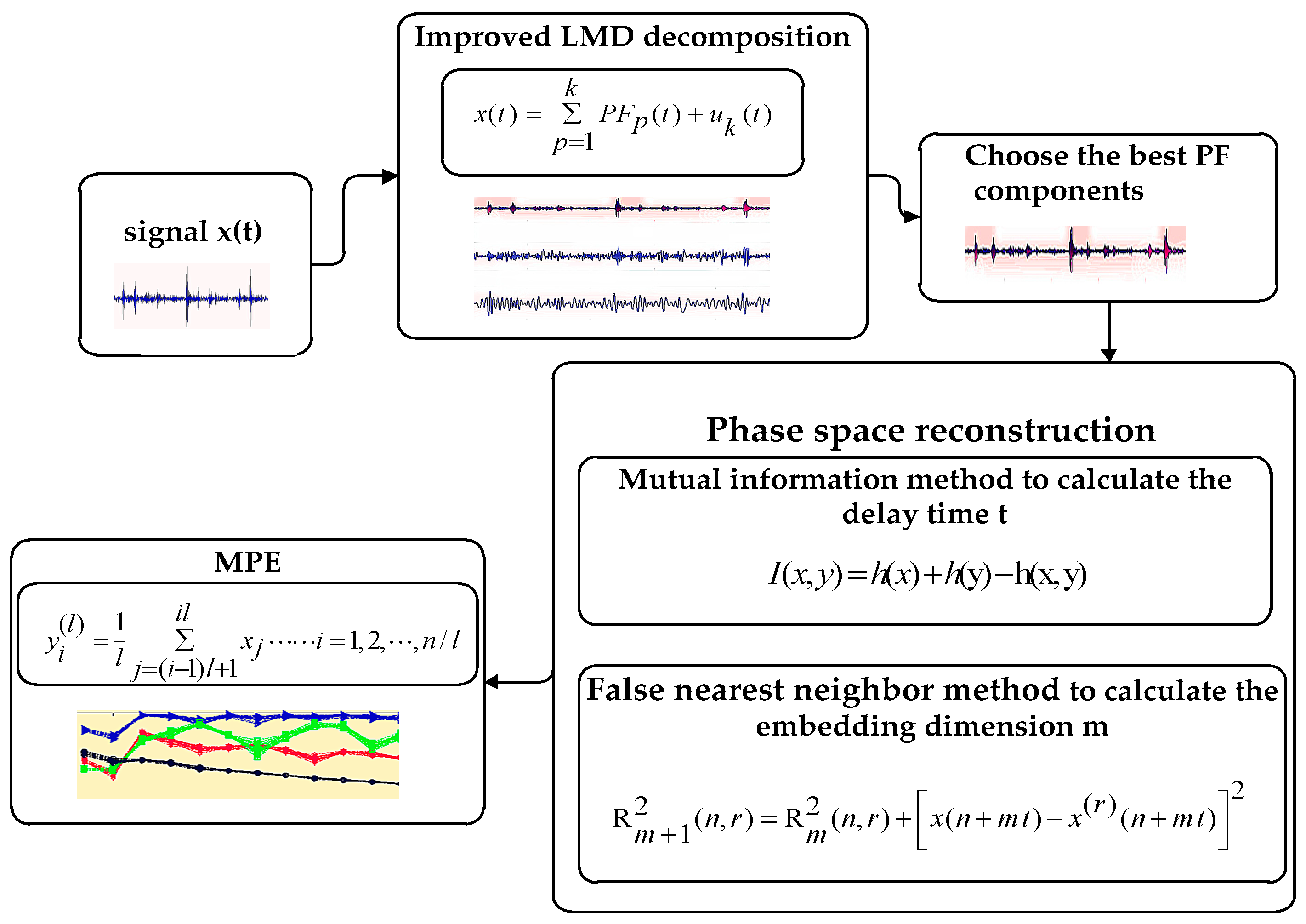
Figure 3.
Mutual information method.
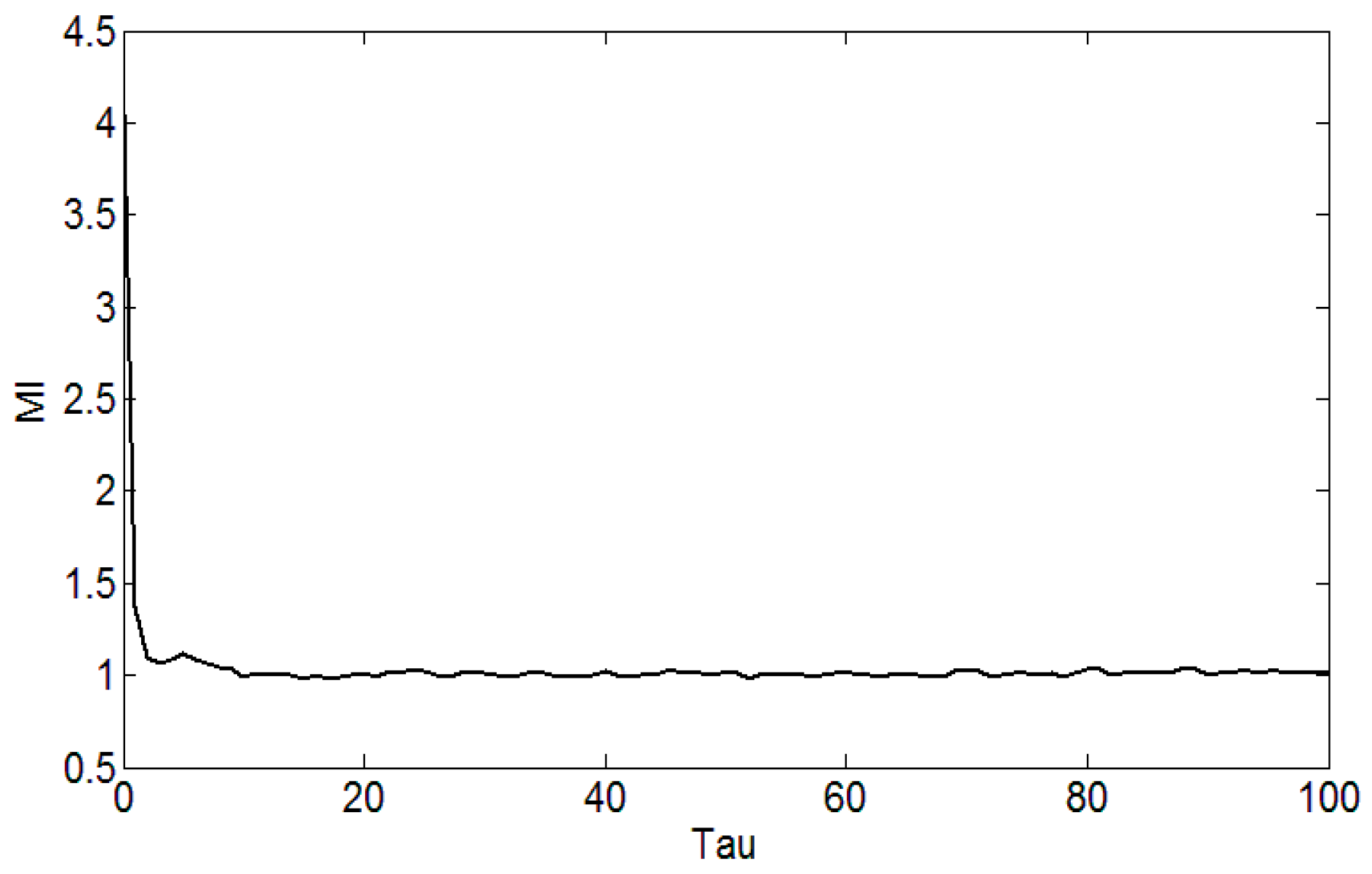
Figure 4.
False nearest neighbor method for Embedding Dimension.

Figure 5.
Diagnosis Flow Based on Hidden Markov Model (HMM).
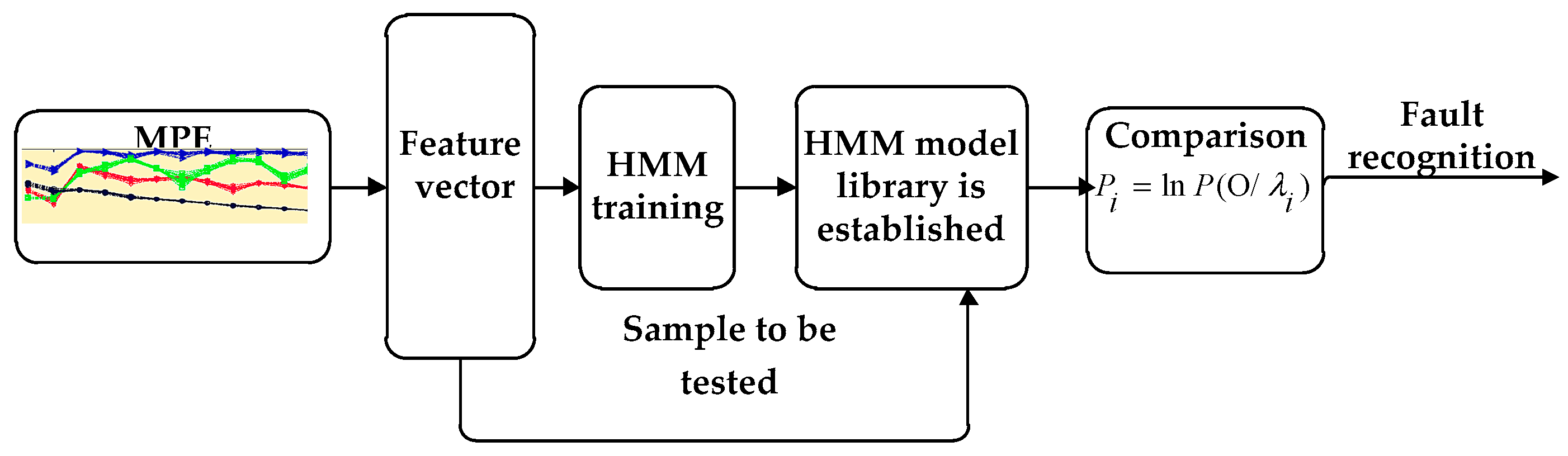
Figure 6.
The rolling bearing experiment system.
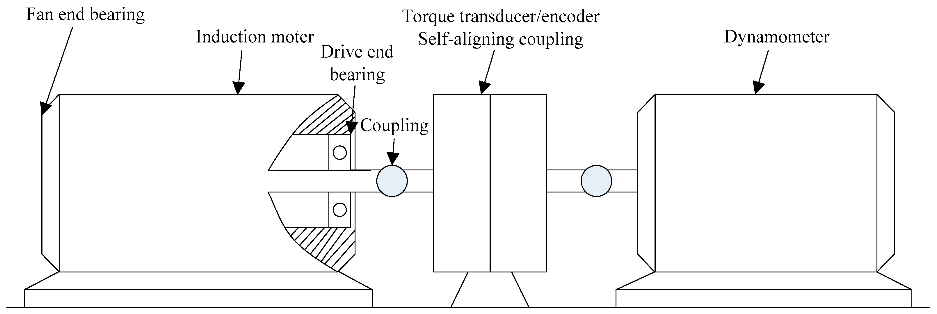
Figure 7.
Inner fault is decomposed by improved LMD.
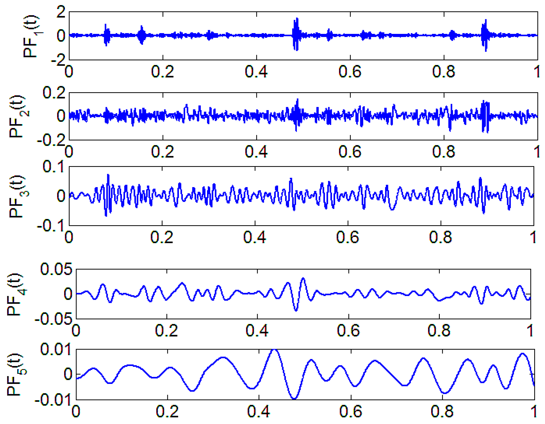
Figure 8.
(a) MPE of four faults; (b) MPE of PF2.

Figure 9.
Number of HMM iterations.

Table 1.
The partial delay time and the embedding dimension.
| Section | BF | OBF | IBF | Normal |
|---|---|---|---|---|
| t | 1 | 1 | 1 | 2 |
| m | 6 | 4 | 5 | 7 |
Table 2.
The part of the sample to be tested identifies the result.
| Fault Condition | Logarithm Likelihood Probabilities of the Input Sample Model | ||||
|---|---|---|---|---|---|
| λ1 | λ2 | λ3 | λ4 | Recognition Result | |
| BF | −9.75854 | −24.5979 | λ1 | ||
| OBF | −157.594 | −15.1449 | λ2 | ||
| IBF | −55.9402 | −9.33311 | −792.054 | λ3 | |
| Normal | −24.0932 | −59.6398 | −5.63077 | λ4 | |
Table 3.
Comparison of improved LMD for Fault Recognition.
| Recognition Model | BF | OBF | IBF | Normal | Recognition Rate | |
|---|---|---|---|---|---|---|
| Improved LMD | HMM | 5 | 5 | 4 | 5 | 95.0% |
| BP | 5 | 4 | 5 | 4 | 90.0% | |
| LMD | HMM | 5 | 4 | 4 | 5 | 90.0% |
| BP | 5 | 4 | 4 | 4 | 85.0% | |
© 2017 by the authors. Licensee MDPI, Basel, Switzerland. This article is an open access article distributed under the terms and conditions of the Creative Commons Attribution (CC BY) license (http://creativecommons.org/licenses/by/4.0/).
Share and Cite
MDPI and ACS Style
Gao, Y.; Villecco, F.; Li, M.; Song, W. Multi-Scale Permutation Entropy Based on Improved LMD and HMM for Rolling Bearing Diagnosis. Entropy 2017, 19, 176. https://doi.org/10.3390/e19040176
AMA Style
Gao Y, Villecco F, Li M, Song W. Multi-Scale Permutation Entropy Based on Improved LMD and HMM for Rolling Bearing Diagnosis. Entropy. 2017; 19(4):176. https://doi.org/10.3390/e19040176
Chicago/Turabian StyleGao, Yangde, Francesco Villecco, Ming Li, and Wanqing Song. 2017. "Multi-Scale Permutation Entropy Based on Improved LMD and HMM for Rolling Bearing Diagnosis" Entropy 19, no. 4: 176. https://doi.org/10.3390/e19040176
Note that from the first issue of 2016, this journal uses article numbers instead of page numbers. See further details here.