
Entropy “2”-Soft Classification of Objects

1
Institute for Systems Analysis of Federal Research Center “Computer Science and Control”, Moscow 117312, Russia
2
Intelligent Technologies in System Analysis and Management, National Research University Higher School of Economics, Moscow 125319, Russia
3
Department of Software Engineering, ORT Braude College, Karmiel 2161002, Israel
*
Author to whom correspondence should be addressed.
Entropy 2017, 19(4), 178; https://doi.org/10.3390/e19040178
Submission received: 10 March 2017
/
Revised: 10 April 2017
/
Accepted: 18 April 2017
/
Published: 20 April 2017
(This article belongs to the Special Issue Maximum Entropy and Its Application II)
Abstract
:A proposal for a new method of classification of objects of various nature, named “2”-soft classification, which allows for referring objects to one of two types with optimal entropy probability for available collection of learning data with consideration of additive errors therein. A decision rule of randomized parameters and probability density function (PDF) is formed, which is determined by the solution of the problem of the functional entropy linear programming. A procedure for “2”-soft classification is developed, consisting of the computer simulation of the randomized decision rule with optimal entropy PDF parameters. Examples are provided.
1. Introduction
The problem of object classification is highly relevant in contemporary theoretical and applied science. Objects, which are subject to classification, can be text documents, audio, video and graphic objects, events, etc. The "m"-soft classification means the attribution of the object to the appropriate m class with a certain probability, unlike the "m"-hard classification, when no alternative distribution of objects by classes is performed. Here, we consider “2”-soft classification, which is the basis for the classification by m classes.
“2”-soft classification is useful in many applied problems, with the exception, perhaps, of “ideal” ones, where all classes, object specification, and data are absolutely accurate. The fact is that real classification problems are immersed in significantly undefined environments. When it comes to data, they are received with errors, omissions, questionable reliability, and different timelines. The formation of decision rule models and their parameterization is not a formalized and subjective process, depending on the knowledge and experience of a researcher. By minimizing an empirical risk of decision rule model in the learning process, we get parameter evaluations for the existing amounts of data (precedents) and for the accepted parameterized model, i.e., evaluations are conditional. How will they, and consequently results of the classification, would behave with other precedents and with other parameterization model remains unclear. Methods of “2”-soft classification are directed to indicate a possible approach to overcome uncertainty factors. The idea is to make a decision rule randomized, and not arbitrarily randomized, but so that its entropy, as a measure of uncertainty, was at the maximum. It would allow for generating an ensemble of the best solutions at the highest uncertainty.
However, among soft and hard classification, fundamental differences exist: the structures of their procedures are similar and based on a more general concept of machine learning by precedents. A huge amount of work is devoted to this issue. Relevant references to them can be found in monographs [1,2,3,4,5,6,7,8], lectures [9,10] and reviews [11,12,13]. The recent fundamental works [6,14,15] clarify the vast diversity of classification algorithms and its learning procedures.
Within the general concept of machine learning, its modification had been proposed: Randomized Machine Learning (RML) [16]. An idea of the randomization is expanding to data and parameters of decision rules. This means that the model parameters of decision rules and data errors are assumed to be randomized in an appropriate way. The difference from existing machine learning procedures is that RML procedures are built not for optimal evaluations of the model parameters, but their probability density function (PDF) and evaluation of the “worst” data errors of PDF. In the RML, as a criterion of evaluation optimality, generalized information entropy is used, maximization of which was carried out on a set described by the system of empirical balances with collections of learning data.
The principle of maximum entropy has already been used in the domain of machine learning—for example, for speech recognition and text classification problems [17] and even for deep neural net parameters estimation [18]. The main advantage of this technique is its robustness to over-fitting in the presence of data errors within small data sets [19,20]. It is demonstrated by the classification experiments with the additive random noise presented in this paper.
2. Statement of the Problem
Suppose that there are two collections of objects: , which must be distributed between two classes. Objects in both collections are performed by vectors, whose components are variable features that characterize an object and measured quantitatively:
We will assume that dimensions of the vectors in both collections are the same, i.e., . Collection is used for learning, and collection for its classification and testing.
The objects in both collections are marked by belonging to a corresponding class: if object or belongs to the first class, it will be assigned 1, or 0 if it belongs to the second one. Consequently, the learning collection is characterized by a vector of answers with components equal to 0 or 1, and a testing collection to vector of responses (at the end of last century it was known as learning with a teacher [2]). Numbers of these vector components correspond to object numbers in learning and testing collections.
2.1. Learning
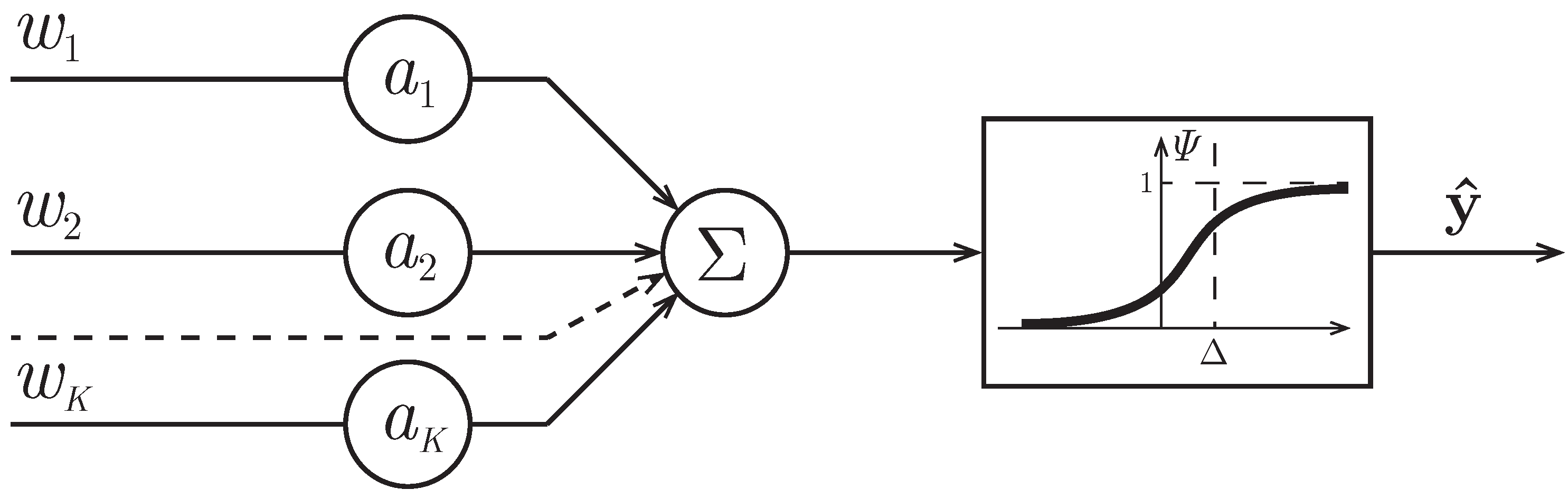
Availability of learning collection allows for hypothesizing about the existence of function (decision rule) . The learning problem is to determine parameterized function , which approximately describes function F. Function characterizes the model of decision rule. Being under the “soft” classification, the randomized model occurs as a model of decision rule, i.e., it has randomized parameters . Its input are vectors , and the output depends on randomized parameters of . As such, we choose a model of a single-layer neural net [21]:
where
Figure 1 shows a graph of the sigmoid function with parameters: “slope” and “threshold” . The function of in the interval corresponds to the first class and the values in the interval -to the second class.
Their probabilistic properties are characterized by PDF , which is defined over set .
Since parameters are random, then for each object , an ensemble of random numbers occurs for the interval . We define it as an average:
Therefore, according to RML [16] general procedure, the problem of “2”-soft classification is represented as follows:
when
where belongs to class of continuously differentiable functions. This is a problem of functional entropy-linear programming, which has an analytical solution, such as entropy optimal PDF , parameterized by Lagrange multipliers :
where is defined by the Equality (2), and
Lagrange multipliers are determined from the Equation (8).
2.2. Testing
At this point, a collection of objects is used, which are characterized by the vector of responses with known objects belonging to grade 1 or 2. Vector will be used to evaluate the quality of testing. In the testing procedure itself, only objects collection will be used.
The subject of the testing is randomized decision Rules (2) and (3) with entropy optimal PDF function of parameters. At the same time, a trial sequence of Monte Carlo is implemented with volume N, every one of which is generated by a random vector with appropriate entropy optimal PDF function (6)–(8). Assume that, as a result of these tests, it was found that the first object from the testing collection was assigned to the first class times and times to the second class; .... k-th object was assigned to the first class times and –to the second class, etc. For a sufficiently large number of tests, the empirical probability can be determined
Therefore, the testing algorithm can be represented as follows (where i is the number of the object):
Step 1-i. In accordance with the optimal PDF function, a set of output values is generated with entropy optimal Models (2) and (3), comprising N random numbers from an interval .
Step 2-i. If the random number from this set is larger than , then the object belongs to the class 1. If it is less than , then it belongs to class 2.
Step 3-i Empirical probabilities are determined (11).
As a result of the functioning of this procedure, any object can be defined in one of two classes with a certain probability, which reflects an uncertainty within data and models of decision rule.
The transition to a hard classification can be accomplished by fixing the threshold of probabilities, an object which above it belongs to the relevant class. The number of objects that can be “hard”-classified depends on the threshold value. It is not difficult to find that when thresholds are greater than 0.5, not all objects are classified, but with more than 0.5 probability. However, at thresholds less than 0.5, all are classified, but with less than 0.5 probability.
3. Model Examples of “2”-Soft Classification
In this section, we present the model experiments conducted in accordance with the proposed learning algorithm. It should be noted that all data sets are synthetic and generated manually with a standard random number generator. The first series of experiments aims to introduce the proposed computational procedure and should be considered as illustrative examples. On the other hand, the last example in the next section is more important and demonstrates the advantages of the probabilistic approach for classification in the presence of data errors.
3.1. Soft “2”-Classification of Four-Dimensional Objects
Consider that the objects characterized by four features are coordinates of vectors and .
3.1.1. Learning
The learning collection consists of three objects, every one of which is described by four attributes, and the values of which are shown in Table 1.
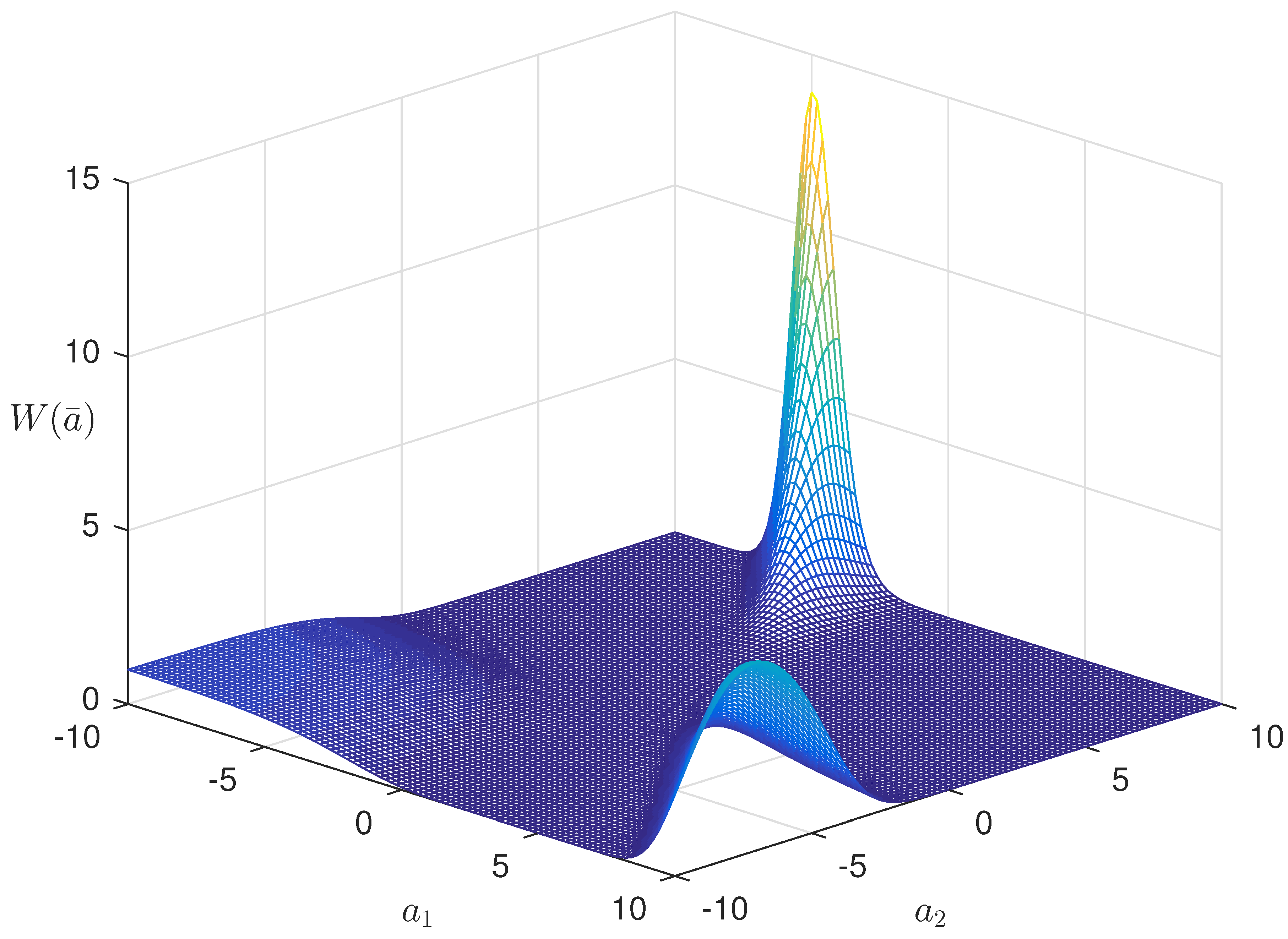
Randomized model of decision Rules (2) and (3) has parameters: and . Learning vector (“teacher’s” answers) ( corresponds. to class 2; corresponds to class 1). Lagrange multipliers for the entropy-optimal PDF (9) have the following values: . Parameters . Entropy-optimal PDF function for this learning collection is as follows:
Figure 2 shows a two-dimensional section PDF .
3.1.2. Testing
At this stage, a set of objects is used, where each element of the set is characterized by vector . The generated array of four-dimensional random vectors , with independent components evenly distributed in intervals . Then, the algorithm of “2”-soft classification is applicable. Figure 3 shows the empirical probabilities of belonging of -object to Classes 1 and 2.
3.2. Two-Dimensional Objects “2”-Soft Classification
Consider the objects characterized by two features that are coordinates of the vectors and .
3.2.1. Learning
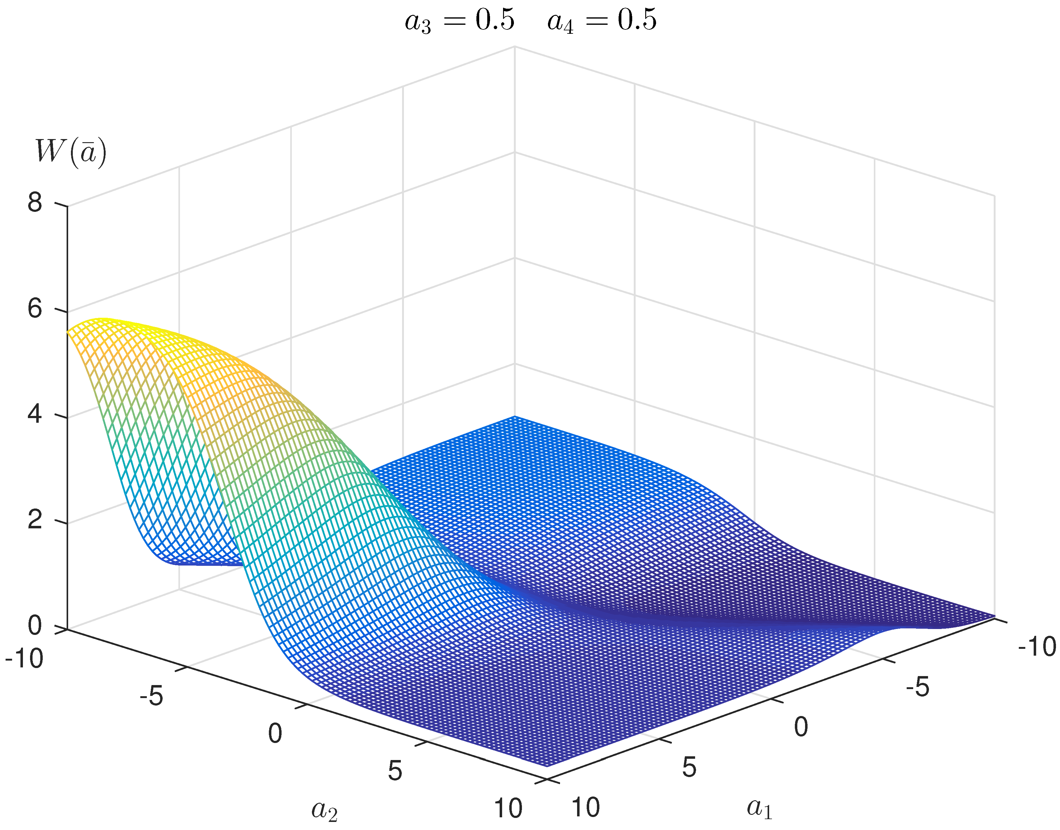
The learning collection consists of three objects, every one of which is described by two attributes, and the values of which are shown in Table 1. The values of parameters and intervals for random parameters correspond to Example 1. Lagrange multipliers for the entropy-optimal PDF (9) have the following values: . Entropy-optimal PDF function for this learning collection is as follows:
Figure 4 shows function .
3.2.2. Testing
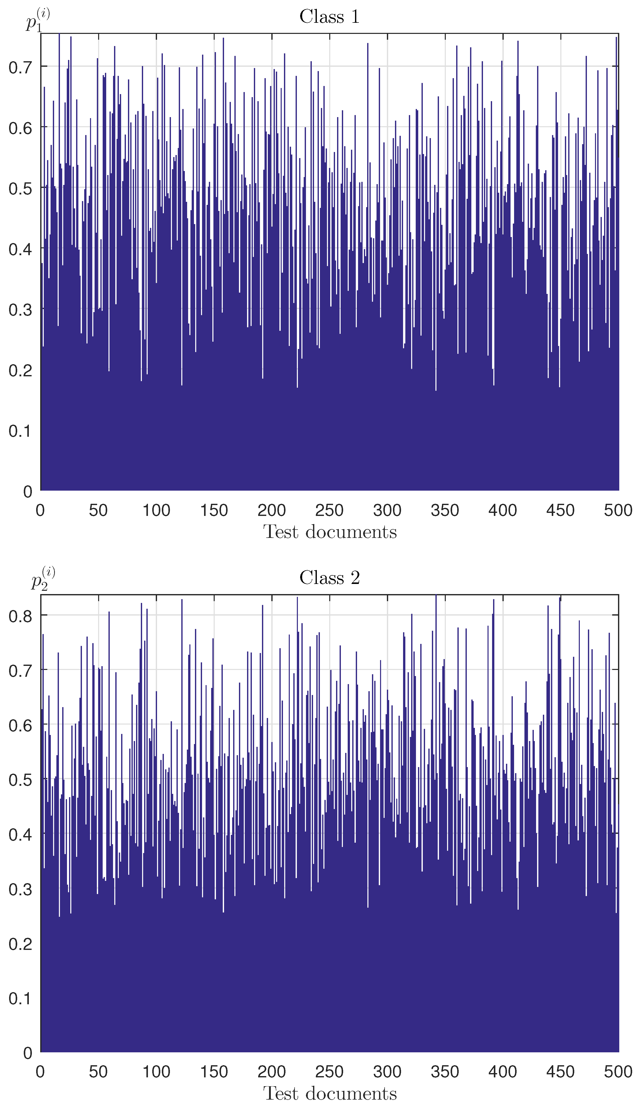
All parameters of this example correspond to Example 2. Figure 5 shows empirical probabilities of belonging of the -object to Classes 1 and 2 ().
4. Experimental Studies of “2”-Hard/Soft Classifications in Presence of Data Errors
“2”-soft classification, based on entropy randomization decision rules, creates a family of “2”-hard classifications, parameterized by thresholds of belonging probabilities. This family complements “2”-hard classifications based on machine learning methods, particularly using the method of least squares [9].
4.1. Data
The experimental study of the soft and hard classifications was performed on simulated data with model errors. All the data for the objects were labeled in order of belonging to one of two classes. This information was used for learning the model of decision rule, and during the method testing to evaluate the classification accuracy.
The objects of classification are characterized by four-dimensional vectors:
Vectors of both collections were chosen in a random order, and they were evenly distributed on a four-dimensional unit cube. Data errors are modeled by random and evenly distributed four-dimensional vectors , where .
To mark the belonging of vectors to one of the two classes, the number generation procedure from interval is applied as follows:
where
Let us recall that the values of the sigmoid function from interval correspond to the first class, and from interval to the second class, i.e.,
Thus, numerical characteristics of objects components of vectors serve as their features, and values refer them to a certain class.
Two collections were formed from these objects: the learning one and the testing one .
4.2. Randomized Model (Decision Rule)
In the experimental study, we used a model that coincides by its structure with (15) and (16), but has randomized parameters and noises:
where are randomized parameters of the interval type. For example, ; is a random interval type noise, i.e., . Noise probabilities are characterized by PDF , which exists as a continuously differentiable function.
The optimization problem of entropy-robust estimation is formulated as follows [16]:
under constraints:
and
In this example, the optimization was performed by MATLAB 2015b software (Version 8.6, Build 267246), using the optimization tools (optimization toolbox) and statistical learning (statistic and machine learning toolbox). The values obtained for Lagrange multipliers are: .
Figure 6 shows a two-dimensional section of entropy-optimal PDF function .
4.3. Testing of Learning Model: Implementation of “2”-Soft Classification
The process of randomized classified algorithm testing involves a generation of a random set of model parameters according to received entropy-optimal density functions. To generate an ensemble of random values, an algorithm of Metropolis–Hastings is used [22].
In this example, the vectors set was generated , with entropy-optimal PDF (22), defining 100 implementations of decision rule classification models. For each object from the testing collection, we obtain an ensemble of numbers from the interval
Along this ensemble, the objects are distributed into classes in accordance with rule
The probabilities of belonging to Classes 1 and 2 are calculated as follows:
Here, and are the numbers of tests in which the objects were classified as Classes 1 and 2, respectively. Figure 7 shows the value distribution of empirical probability of belonging to Classes 1 and 2 for testing sample objects, which characterize “2”-soft classification with entropy optimal linear decision rule.
It was noted above that with “2”-soft classification, you can generate families of “2”-hard classification, assigning various thresholds of empirical probability. Belonging to a class is defined by the following condition:
Let us determine the accuracy of classification as:
where L is the length of the test collection, and is the number of correct classifications.
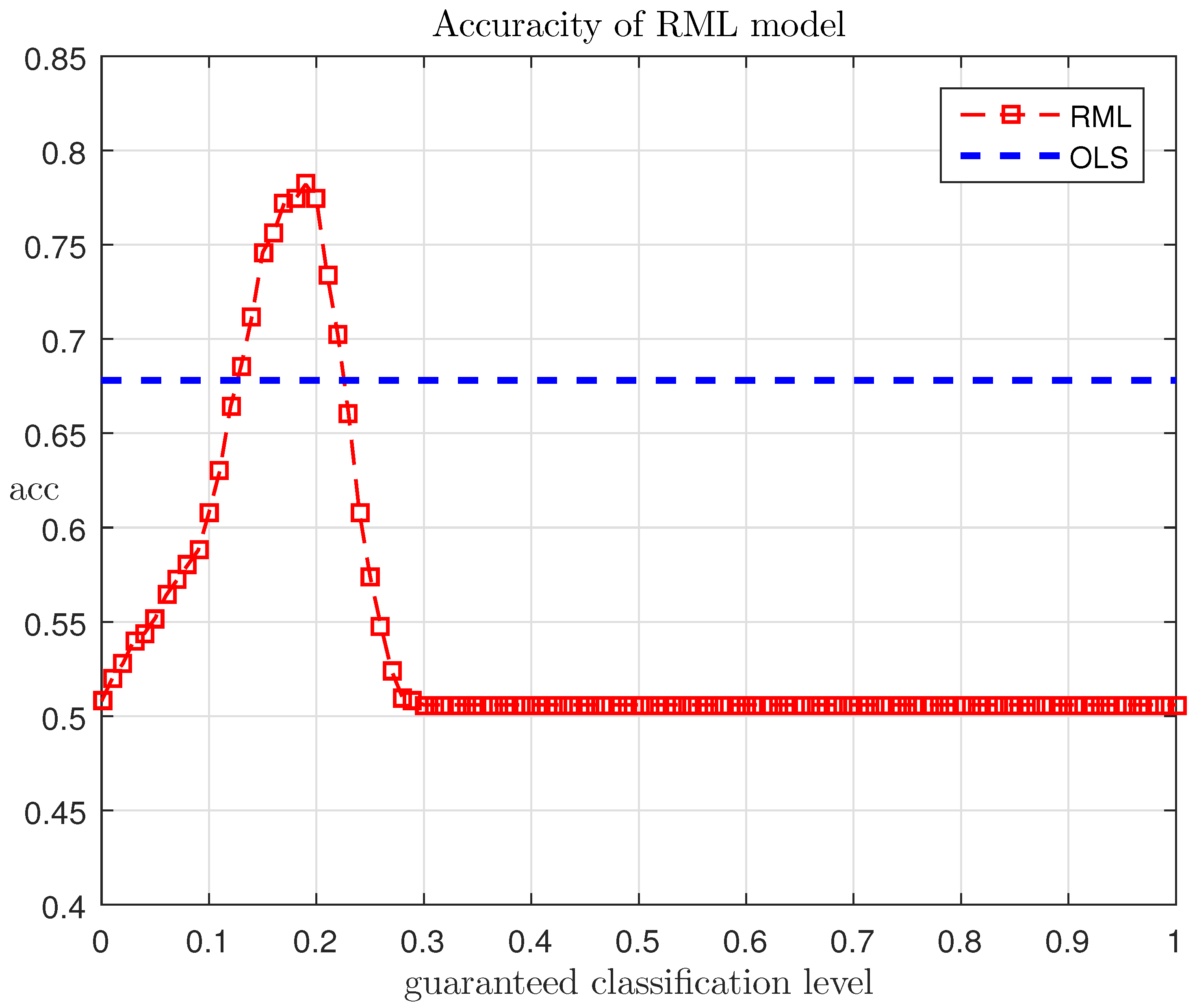
The research of the above example shows the existence of dependence between the accuracy and the threshold . Figure 8 shows this dependence, where we can see that the quantity attains a maximum value equal to 78.5% at . However, “2” hard classification, which uses the decision rule (26) with non-randomized parameters and the method of least squares to determine their values, yields a 66% accuracy (regardless of the threshold).
This result means that a traditional exponential model widely used for classification problems [6,9] could be improved by statistical interpretation of its output. In this case, the proposed randomized machine learning technique that evolves the generation of entropy-optimal probability functions, and variation of soft decision threshold boosts the accuracy of classification to nearly 80 percent.
5. Conclusions
A method for “2”-soft classification was proposed, which allows for referring objects with calculated empirical probability to one of two classes. The latter is determined by the Monte Carlo method with the use of the entropy-optimal randomized model of the decision rule. A corresponding problem is formulated for the maximization of entropy functional on the set, a configuration of which is determined by balances between the real input data and average output of the randomized model of the decision rule.
The problem of “2”-soft classification for the case of existence of data errors simulated by the additive noise evenly distributed in the parallelogram. The entropy-optimal estimations of probability distribution density for model parameters and for noises, which are the best at the maximum indeterminateness in terms of entropy, were obtained. We performed an experimental comparison of “2”-hard and “2”-soft classifications. An existence of the classification threshold interval was revealed, whereby a precision of “2”-soft classification (the number of correct answers) was increased by 20. Examples illustrating the proposed method are provided.
Acknowledgments
This work was supported by the Russian Foundation for Basic Research (Project No. 16-07-00743). We also thank the comments from the two anonymous reviewers, which improved the quality of the paper.
Author Contributions
Yuri S. Popkov and Zeev Volkovich introduced the ideas of this research, formulated the main propositions and wrote the paper; Yuri A. Dubnov made the experiments; and Renata Avros and Elena Ravve reviewed the paper and provided useful comments.
Conflicts of Interest
The authors declare no conflict of interest.
References
- Rosenblatt, M. The Perceptron—Perceiving and Recognizing Automaton; Report 85-460-1; 1957; Available online: http://blogs.umass.edu/brain-wars/files/2016/03/rosenblatt-1957.pdf (accessed on 19 April 2017).
- Tsipkin, Y.Z. Basic Theory of Learning Systems; Nauka (Science): Moscow, Russia, 1970. [Google Scholar]
- Ayzerman, M.A.; Braverman, E.M.; Rozonoer, L.I. A Potential Method of Machine Functions in Learning Theory; Nauka (Science): Moscow, Russia, 1970. [Google Scholar]
- Vapnik, V.N.; Chervonenkis, A.Y. A Theory of Pattern Recognition; Nauka (Science): Moscow, Russia, 1974. [Google Scholar]
- Vapnik, V.N.; Chervonenkis, A.Y. A Recovery of Dependencies for Empirical Data; Nauka (Science): Moscow, Russia, 1979. [Google Scholar]
- Bishop, C.M. Pattern Recognition and Machine Learning; Series: Information Theory and Statistics; Springer: New York, NY, USA, 2006. [Google Scholar]
- Hastie, T.; Tibshirani, R.; Friedman, J. The Elements of Statistical Learning: Data Mining, Inference, and Prediction; Springer, 2009. Available online: https://statweb.stanford.edu/tibs/ElemStatLearn/ (accessed on 19 April 2017).
- Merkov, A.B. Pattern Recognition. Building and Learning Probabilistic Models; M. LENAND: Moscow, Russia, 2014. [Google Scholar]
- Vorontsov, K.V. Mathematical Methods of Learning by Precedents; The Course of Lectures at MIPT. Moscow, Russia, 2006. Available online: http://www.machinelearning.ru/wiki/images/6/6d/Voron-ML-1.pdf (accessed on 19 April 2017).
- Zolotykh, N.Y. Machine Learning and Data Analysis. 2013. Available online: http://www.uic.unn.ru/zny/ml/ (accessed on 19 April 2017).
- Boucheron, S.; Bousquet, O.; Lugosi, G. Theory of Classification: A Survey of Some Recent Advances. ESAIM Probab. Stat. 2005, 9, 323–375. Available online: http://www.esaim-ps.org/articles/ps/pdf/2005/01/ps0420.pdf (accessed on 19 April 2017). [CrossRef]
- Smola, A.; Bartlett, P.; Scholkopf, B.; Schuurmans, D. Advances in Large Margin Classifiers; MIT Press: Cambridge, MA, USA, 2000. [Google Scholar]
- Jain, A.; Murty, M.; Flunn, P. Data Clustering: A Review. ASM Comput. Surv. 1999, 31, 264–323. [Google Scholar] [CrossRef]
- Brown, G. Ensemble learning. In Encyclopedia of Machine Learning; Sammut, C., Webb, G.I., Eds.; Springer: New York, NY, USA, 2010; pp. 312–320. [Google Scholar]
- Furnkranz, J.; Gamberger, D.; Lavrac, N. Foundations of Rule Learning; Springer: Berlin/Heidelberg, Germany, 2012. [Google Scholar]
- Popkov, Y.S.; Dubnov, Y.A.; Popkov, A.Y. Randomized Machini Learning: Statement, Solution, Applications. In Proceedings of the IEEE International Conference on Intelligent Systems, Sofia, Bulgaria, 4–6 September 2016. [Google Scholar]
- Kamal, N.; John, L.; Andrew, M. Using Maximum Entropy for Text Classification. IJCAI-99 Workshop on Machine Learning for Information Filtering. Available online: http://www.cc.gatech.edu/isbell/reading/papers/maxenttext.pdf (accessed on 19 April 2017).
- Payton, L.; Fu, S.-W.; Wang, S.-S.; Lai, Y.-H.; Tsao, Y. Maximum Entropy Learning with Deep Belief Networks. Entropy 2016, 18, 251. [Google Scholar]
- Amos, G.; George, G.; Judge, D.M. Maximum Entropy Econometrics: Robust Estimation with Limited Data; John Wiley and Sons Ltd.: Chichester, UK, 1996; p. 324. [Google Scholar]
- Japkowicz, N.; Shah, M. Evaluating Learning Algorithms: A Classification Perspective; Cambridge University Press: Cambridge, UK, 2011. [Google Scholar]
- Gerstner, W.; Kishler, W.M. Spiking Neuron Models: Single Neurons, Population, Plasticity; Cambridge University Press: Cambridge, UK, 2002. [Google Scholar]
- Rubinstein, R.Y.; Kroese, D.P. Simulation and Monte Carlo Method; John Willey and Sons: Hoboken, NJ, USA, 2008. [Google Scholar]
Figure 1.
Structure of a single-layer neural net.

Figure 2.
Two-dimensional section of probability density function (PDF) .

Figure 3.
The empirical probabilities for example 1.

Figure 4.
Entropy-optimal PDF function .

Figure 5.
The empirical probabilities for example 2.
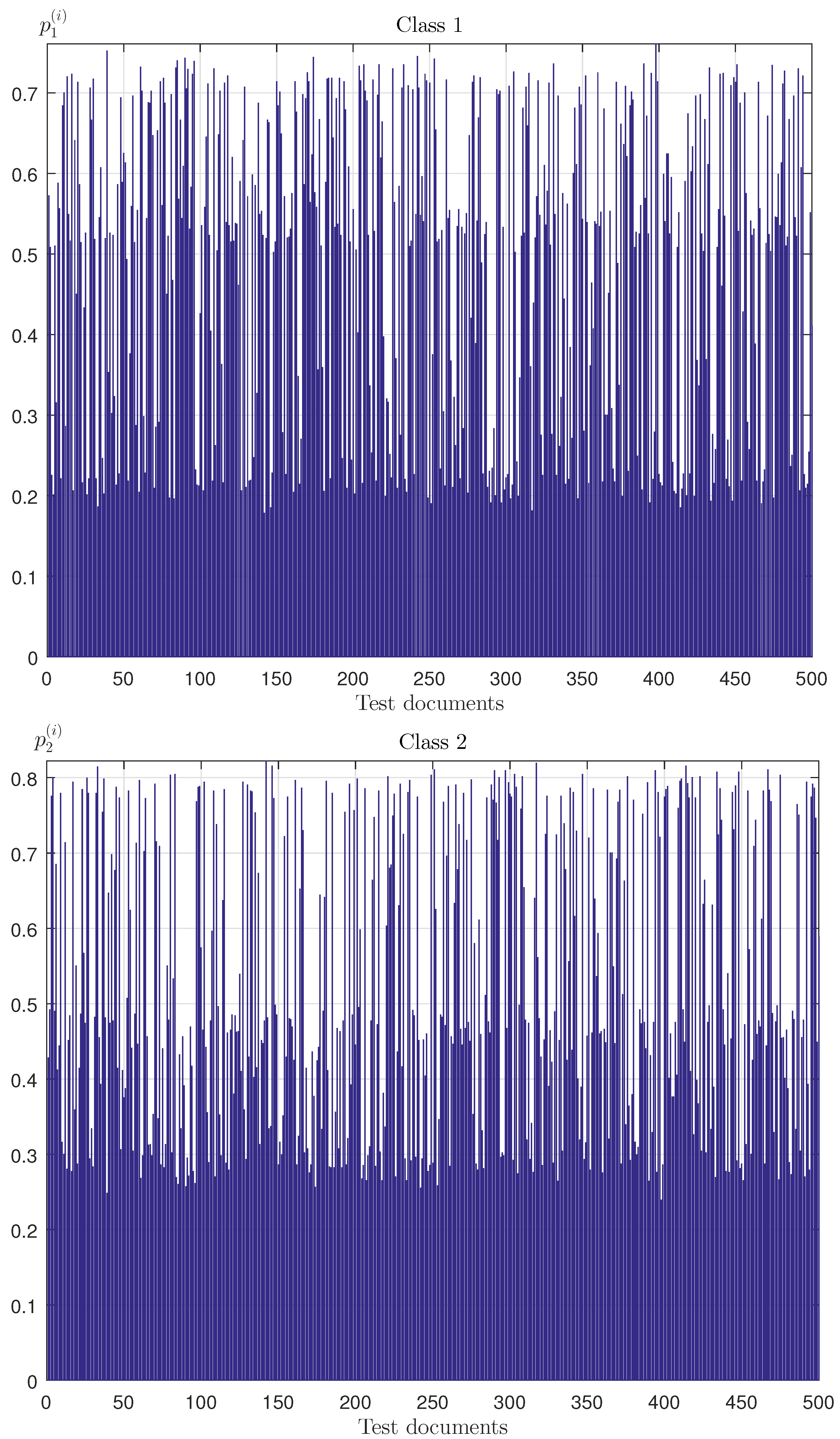
Figure 6.
Two-dimensional section of function .
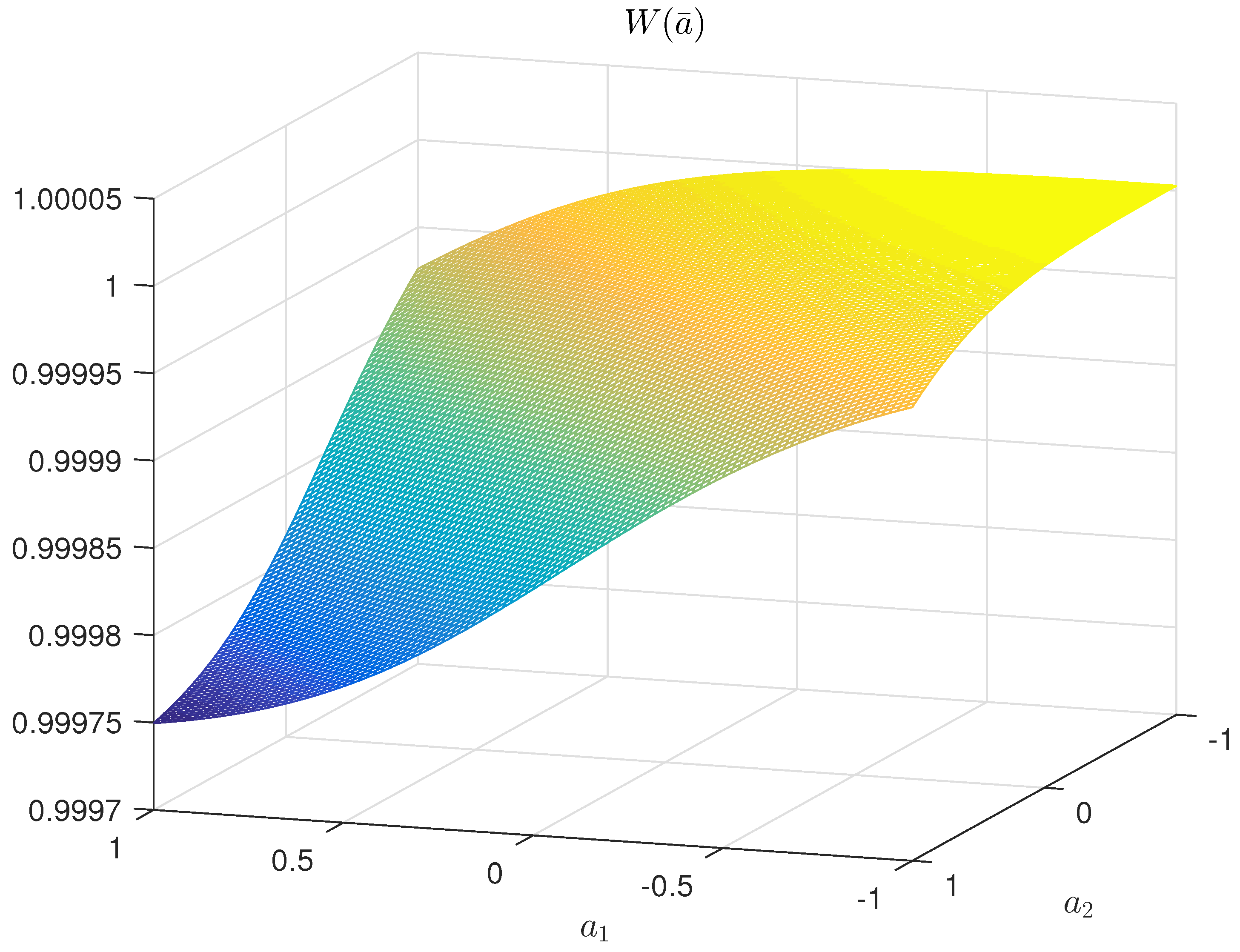
Figure 7.
The empirical probabilities of belonging to classes 1 and 2.
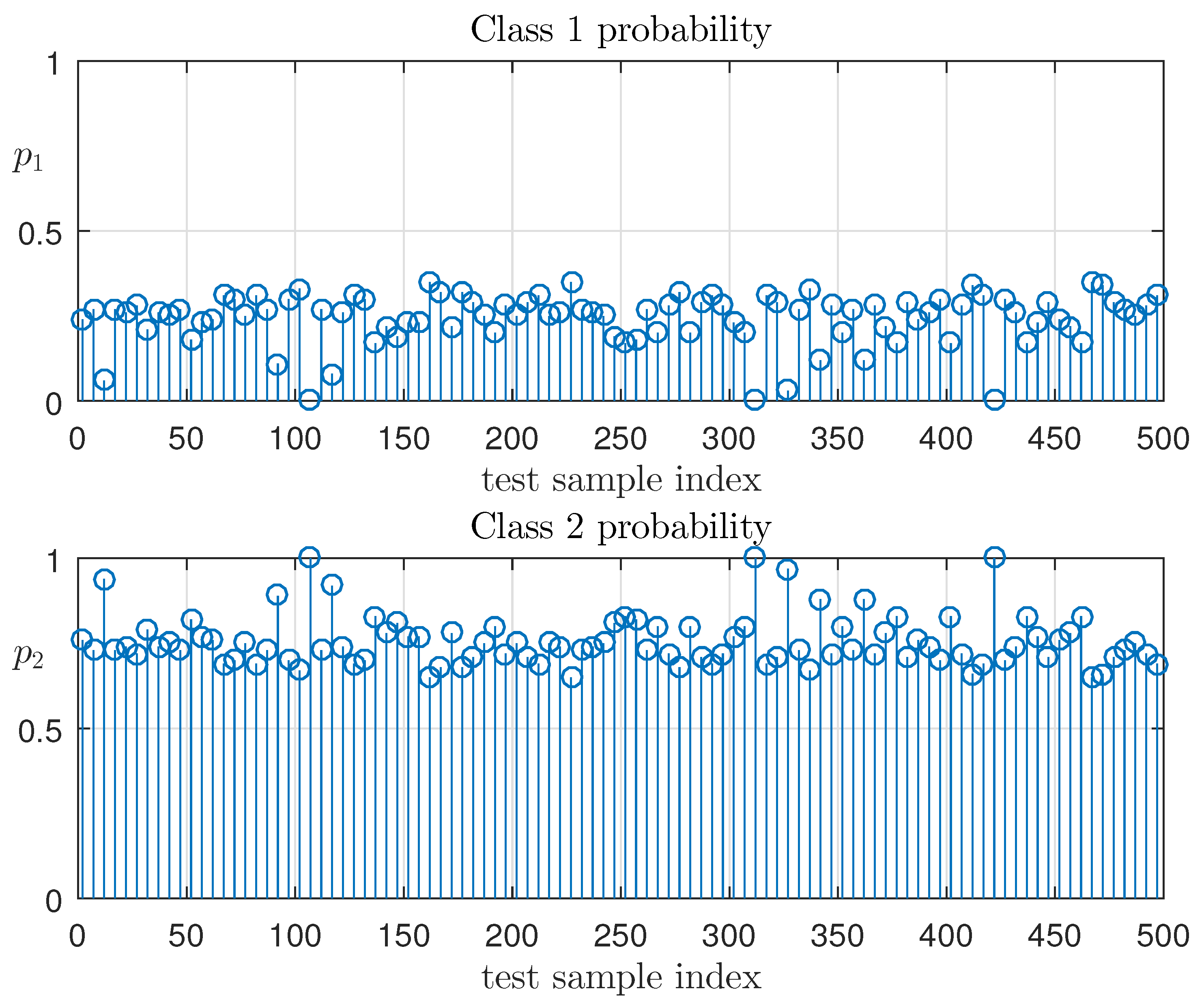
Figure 8.
Dependence of RML model accuracy on the threshold .

Table 1.
Learning data example.
| i | ||||
|---|---|---|---|---|
| 1 | 0.11 | 0.75 | 0.08 | 0.21 |
| 2 | 0.91 | 0.65 | 0.11 | 0.81 |
| 3 | 0.57 | 0.17 | 0.31 | 0.91 |
© 2017 by the authors. Licensee MDPI, Basel, Switzerland. This article is an open access article distributed under the terms and conditions of the Creative Commons Attribution (CC BY) license (http://creativecommons.org/licenses/by/4.0/).
Share and Cite
MDPI and ACS Style
Popkov, Y.S.; Volkovich, Z.; Dubnov, Y.A.; Avros, R.; Ravve, E. Entropy “2”-Soft Classification of Objects. Entropy 2017, 19, 178. https://doi.org/10.3390/e19040178
AMA Style
Popkov YS, Volkovich Z, Dubnov YA, Avros R, Ravve E. Entropy “2”-Soft Classification of Objects. Entropy. 2017; 19(4):178. https://doi.org/10.3390/e19040178
Chicago/Turabian StylePopkov, Yuri S., Zeev Volkovich, Yuri A. Dubnov, Renata Avros, and Elena Ravve. 2017. "Entropy “2”-Soft Classification of Objects" Entropy 19, no. 4: 178. https://doi.org/10.3390/e19040178
Note that from the first issue of 2016, this journal uses article numbers instead of page numbers. See further details here.