
Using Measured Values in Bell’s Inequalities Entails at Least One Hypothesis in Addition to Local Realism

Centro de Investigaciones en Láseres y Aplicaciones (CEILAP), UNIDEF (MINDEF-CONICET), CITEDEF, J.B. de La Salle 4397, Villa Martelli 1603, Argentina
Entropy 2017, 19(4), 180; https://doi.org/10.3390/e19040180
Submission received: 22 February 2017
/
Revised: 17 April 2017
/
Accepted: 20 April 2017
/
Published: 22 April 2017
(This article belongs to the Special Issue Foundations of Quantum Mechanics)
Abstract
:The recent loophole-free experiments have confirmed the violation of Bell’s inequalities in nature. Yet, in order to insert measured values in Bell’s inequalities, it is unavoidable to make a hypothesis similar to “ergodicity at the hidden variables level”. This possibility opens a promising way out from the old controversy between quantum mechanics and local realism. Here, I review the reason why such a hypothesis (actually, it is one of a set of related hypotheses) in addition to local realism is necessary, and present a simple example, related to Bell’s inequalities, where the hypothesis is violated. This example shows that the violation of the additional hypothesis is necessary, but not sufficient, to violate Bell’s inequalities without violating local realism. The example also provides some clues that may reveal the violation of the additional hypothesis in an experiment.
1. Introduction
Bell’s inequalities [1] are correlation bounds between results of measurements performed on two remote particles. They are derived by consistently following a classical description of an experiment like the one in Figure 1. This classical description holds to the innate ideas of locality (roughly speaking: the results of an experiment are independent of the events outside its past lightcone) and realism (roughly speaking: the properties of the physical world are independent of whether it is being observed or not). From these two innate ideas, two specific properties are derived: measurement independence, which means that the values of an hypothetical (“hidden”) variable carried by the particles are uncorrelated from the setting of the observation apparatus (the α,β angles in Figure 1) and counterfactual definiteness, which means that it is possible to assign values to the results of non-performed observations. For example, in the case of the setup in Figure 1, one of the bounds most used in the experiments is the Clauser–Horne–Shimony and Holt (CHSH) inequality, which reads
where the E(α,β) are expectation values defined as
and the Cij are the number of coincidences observed at the detectors, where i,j = + (−) label the transmitted (reflected) output of the analyzer and the first (second) index indicates the A (B) station. The |α,β on the right means that all the coincidences have been recorded with the analyzers set to the angle values {α,β}. Then, for example, C+−|0,π/8 is the number of coincidences recorded with a photon detected in the transmitted output of the analyzer at Station A and the reflected output at Station B, when the angle setting is 0 at A and π/8 at B. The predictions of quantum mechanics (QM) violate Equation (1). For example, for the entangled state of two particles |ϕ+〉 = (1/√2){|xa,xb〉 + |ya,yb〉}, if {α,β,α’,β’} are chosen to be equal to {0,π/8,π/4,3π/8}, then SCHSH = 2√2 > 2. This prediction (or others alike) has been experimentally confirmed under rigorous conditions [2,3,4,5,6,7,8,9,10]. The apparent conclusion is that locality and/or realism (in short: local realism, LR) are not valid in nature. This contradiction is a crucial issue, because LR is assumed not only in everyday life, but also in all scientific practice (excepting QM, of course). The contradiction should hence be solved in a fully satisfactory way in order to attain a coherent approach to the study of nature.
SCHSH ≡ |E(α,β) − E(α,β’)| + |E(α’,β’) +E(α’,β)| ≤ 2
Nevertheless, a careful analysis shows that at least one additional hypothesis is necessary to insert the results of real measurements into Bell’s inequalities [11]. This additional hypothesis is not the consequence of an experimental imperfection, as in the case of the “loopholes” [1]. The main loopholes are the consequences of a low efficiency detection (often called fair-sampling or detection loophole), of the possibility, in some setups, that the source S knows or can predict the analyzers’ settings (locality, freedom-of-choice, or predictability loophole), of the ambiguity, in some setups, in the definition of coincidences (time-coincidence loophole), or of the possibility that the system evolves depending on earlier outcomes of the observations (memory loophole). Recent experiments [7,8,9,10] have closed these loopholes by using high-efficiency detectors, a space-like separated, random selection of the analyzers’ settings, time-stamped data, and sophisticated statistical analysis. A sort of critical review of these improvements can be found in [12]. Note that the loopholes are of empirical origin, so that the experiments (the performed and the future ones as well) can be modified in favor of closing them. On the other hand, the additional hypothesis involved in the present work is not avoidable by improving or modifying the experiment, since it is the logical consequence of the very nature of any real experiment: the fact that one can register only one reading of the experiment’s output (which includes the definition of the analyzers’ settings in the case of Figure 1) at a time. This fact is not specific to the experiments related with the foundations of QM, but essential to any statistical observation of the real world. In this regard, the statement at the end of Section 2.2, which refers to a weak point in the usual way the theory of probability is applied to the results of observations, is relevant.
In the next few pages, the necessity of the additional hypothesis is discussed with some detail. In order to give a glimpse of its meaning in advance: the additional hypothesis (actually, it is one of a set of hypotheses) is similar to the assumption that the dynamics at the level of the hidden variables is ergodic. Taking into account the importance of the controversy between QM and LR, it seems sensible to speculate that the observed violation of Bell’s inequalities is a refutation of this additional hypothesis, not of LR. This would indicate an elegant solution to the controversy. In addition, as it is discussed at the end of this paper, there is some hope that the validity of the additional hypothesis can be experimentally tested.
In the next section, the reasoning leading to the necessity of an additional hypothesis to retrieve the significance of usual Bell’s inequalities is reviewed. In Section 3, a simple model that violates the additional hypothesis is described. I warn the reader that the aim of this model is not to propose a LR model able to survive the recent experimental results (in fact, it is not), but to study the premises necessary for the validity of Bell’s inequalities. Finally, the design of an experiment able to detect the violation of the additional hypothesis is sketched.
2. The Hypothesis Additional to LOCAL Realism
2.1. Review of the Derivation of the CHSH Inequality
The strength of Bell’s inequalities is that they take into account all the possible ways a classical system can produce correlated results between measurements performed on two remote particles. In order to produce such correlations, each particle is supposed to carry a “hidden variable,” named λ, that influences the process of detection. Therefore, in the case of the CHSH inequality, the observable that corresponds to a coincident detection depends on the angle settings and λ, that is: AB(α,β,λ) ≡ A(α,λ) × B(β,λ) (where A,B = ±1). Then:
and its expectation value is the average over the λ-space:
where ∫dλ × ρ(λ) = 1, ρ(λ) ≥ 0. For the angle settings {α,β} and {α,β’},
adding and subtracting the term [AB(α,β,λ) × AB(α’,β,λ) × AB(α,β’,λ) × AB(α’,β’,λ)] inside the integral, reordering and applying the modulus (note that 1 ± AB ≥ 0) [1]:
which leads to CHSH inequality, Equation (1). Let’s see now why an additional hypothesis is needed to insert the experimental data into this inequality keeping its usual meaning valid.
E(α,β) = ∫dλ × ρ(λ) × AB(α,β,λ)
E(α,β) − E(α,β’) = ∫dλ × ρ(λ) × AB(α,β,λ) − ∫dλ × ρ(λ) × AB(α,β’,λ) = ∫dλ × ρ(λ) × [AB(α,β,λ) − AB(α,β’,λ)]
|E(α,β) − E(α,β’)| ≤ ∫dλ × ρ(λ) × [1 ± AB(α’,β’,λ)] + ∫dλ × ρ(λ) × [1 ± AB(α’,β,λ)] = 2 ± [E(α’,β’) + E(α’,β)]
2.2. The Additional Hypothesis
All real measurements occur successively in time. For example,
represents the following process: set the analyzers’ angles to {α,β} during the time interval [θ,θ + ΔT], sum up the number of coincidences detected after each analyzer’s outputs, and calculate the ratio in Equation (3). Note that E(α,β) in Equation (4) is an average over the space of the hidden variable λ, while E(α,β)measured in Equation (7) is an average over time. In practice, these two averages are implicitly assumed to be equal, but they may not be. The assumption stating that these two averages are equal is the well-known ergodic hypothesis. In other words, Bell’s inequalities are derived from assuming LR, but they can be used in the real world only if ergodicity (or a similar hypothesis, see later) is also assumed. The idea that non-ergodicity may be related with the solution of the QM vs. LR controversy is not new [13,14,15]. Yet, it must be warned that the meaning given to “non-ergodicity” in those early approaches was influenced by the proposal of an LR model based on a system of coupled oscillators (thus similar to the best known example of non-ergodicity: the Fermi–Pasta–Ulam system) [16]. This proposal was eventually shown to be reducible to a form of the time-coincidence loophole [17]. Instead, the meaning given to “non-ergodicity” here is more general.
The historical connection between the terms “non-ergodicity” and “time-coincidence loophole” may lead to confusion. I stress that “non-ergodicity” here has no relationship with the time-coincidence loophole. This loophole is based on a “conspiratorial” modification of photons’ detection times [17]. Somebody might still think that the recent loophole-free experiments are also free from the need of the, as it were, “ergodicity hypothesis,” since they only take into account an outcome for the whole time interval that the measurement lasts, and that fine detail of what happens inside that time interval is ignored. This approach may close the time-coincidence loophole, but it does not avoid the “ergodicity hypothesis.” Note that, at a given time or, if preferred, at the time interval (say) #1234, only one analyzers’ setting is fixed (say {α,β’}, not two or more of the four possible settings, see Figure 1). The result of the observation in time interval #1234 is then saved in only one “box” (say, {−,+,α,β’}, not in 2or more of the 16 possible boxes). When the experimental run ends after summing up the results of many time intervals (say, from #1 to #106), the numbers in the boxes are fatally averages over time, while the terms in the (theoretically derived) Bell’s inequality are averages over the ensemble of states of the hidden variable. Simply, the two averages are not necessarily equal. We cannot insert the numbers in the boxes into the derived Bell’s inequality (and to expect the result to be logically linked to the premises for deriving that inequality) unless we suppose the two averages (time and ensemble) are equal, which is the usual meaning of “ergodicity”.
Now, let us explore the conditions that are necessary to apply Bell’s inequalities as we are used to. We will find that “ergodicity” is only one of the possible hypotheses in a set.
If measurement independence is assumed valid (what is a consequence of assuming locality), then the distribution of the time intervals among the angle settings (that is, if it is a single continuous interval or many separated small intervals, as in the experiments with random varying analyzers [7,8,9,10]) is irrelevant. Let us assume then, for simplicity, that the angle setting at Station A is α from t = 0 to T/2 and α’ from T/2 to T, and at Station B the setting is β’ from t = 0 to T/4 and from t = 3T/4 to T, and β from t = T/4 to 3T/4. A different distribution requires a more involved notation of the integration intervals, but the result is the same. Now the problem in the usual derivation of the CHSH inequality appears clearly in the passage from the first to the second equality in Equation (5), which now becomes
The rhs in the first line of Equation (8) is what is actually measured, while the integral in the second line is the expression that leads to the CHSH inequality. The expressions are different simply because the integration intervals are different. The same happens with the integrals for the term added and subtracted to derive Equation (6) from Equation (5). In consequence, the measured values may violate the CHSH inequality Equation (1) or not but, at this point, this result implies nothing about the validity of LR. This is because the CHSH inequality is derived from the second line of Equation (8), which is different from the measured expression (the first line in Equation (8)). In a few words: the logical link is broken. To restore the logical link it would be necessary to sum all the observables under the same interval of integration. However, going back in time to measure with a different setting to complete the integral is impossible. This is an impossibility from which there is no escape, no matter the inequality or the setup used. One may say, “Well, this is sad, we have worked for so many years for nothing, let’s forget about all this” or, instead, to explore under what hypotheses (in addition to LR) the usual Bell’s inequalities maintain their significance. The key is to bridge the gap between the first and the second lines in Equation (8).
In order to do this, the integrals in the first line in Equation (8) must be completed with expectation values obtained under conditions that did not occur or counterfactual values. This step does not require additional assumptions, since realism, which is already assumed in the derivation of Bell’s inequalities, does allow counterfactual reasoning. The first line of Equation (8) completed in that way is now equal to the second line:
where the underlined terms are the sum of three counterfactual time averages:
For example, the factor AB(α,β,t) indicates the result of a measurement performed at a time value when it actually was B ≠ β, that is, a counterfactual result. By definition, its numerical value is
which is unknown, because all the Cij = 0. It is a zero-over-zero indeterminacy. Yet, counterfactual definiteness ensures that the rhs of Equation (12) does take some value (see later).
The derivation of the CHSH inequality continues as usual, and the final expression is
I stress that it is this Equation (13), not Equation (1), the inequality that is derived by assuming LR only. Equation (13) is not as trivial as it may appear, for the (underlined) counterfactual terms span over three time intervals instead of one (see Equations (10) and (11)), and hence they can be, in principle, as much as thrice as large as the corresponding (non-underlined) factual ones.
As Bell’s inequalities are derived within LR, counterfactual reasoning is acceptable and no additional hypotheses are necessary to derive Equation (13). However, there is now the problem of giving numerical values to the counterfactual terms. In order to solve this problem, a “possible world” must be defined to ensure logical consistency [18]. There is no mystery in this situation, just a lack of information. Let us consider an example from everyday life: Let us suppose that, when I go to the cafeteria and find my friend Alice there, the result of the observable A≡ “I find Alice in the cafeteria” is 1, and 0 when I do not find her there. After many visits to the cafeteria, I measure the expectation value 〈A〉 = 0.3. This is the available information. Now, let us consider the question, “What is the expectation value of A when I don’t go to the cafeteria?” Assuming that Alice and the cafeteria have a well defined existence even when I do not go there (roughly speaking, if realism or counterfactual definiteness is assumed), and then slightly changing the definition of A, from “I find” to “To find,” the expectation value of A is some well defined number, say, q. However, the value of q cannot be known with the information available at this point. More information is needed regarding the behavior of Alice and the properties of the cafeteria when I am not observing them (that is, a “possible world” must be defined) to assign a numerical value to q. Defining this missing information means a hypothesis in addition to LR. If this additional hypothesis is not made (that is, if this missing information is not provided), then the values of the counterfactual terms in Equation (13) (which cannot be measured) remain undefined, and it is therefore impossible to know whether or not the results of an experiment (which measures only the factual terms) violate the inequality.
Once a possible world is defined, the counterfactual terms can be calculated. Depending on the possible world chosen, Equation (1) is retrieved from Equation (13), or not [11]. I stress that the important point here is this: the definition of a possible world unavoidably entails one assumption in addition to LR. This weakens the consequences of the violation of Bell’s inequalities reported in the experiments, for the violation can be interpreted as a refutation of the additional assumption, not necessarily of LR. Note that this weakening is not due to an experimental imperfection, as in the case of the loopholes. The setup in Figure 1 is assumed ideally perfect. The weakening is a consequence of the fact that real measurements are performed in time, and that it is impossible to measure with two different angle settings at the same time. It seems to be related to a weak point in the usual way the theory of probability is applied to the results of observations. In the usual way, events are thought to occur in abstract, independent parallel worlds. The average over an ensemble of these parallel worlds allows the simple calculation of probabilities. In any actual observation instead, events occur (and averages are obtained) successively in time, in the only available real world. The difference between these two situations is at the core of the recent resolution of a paradox in gambling theory [19,20].
2.3. The Conditions for Retrieving the Validity of Bell’s Inequalities
The simplest way to retrieve Equation (1) from Equation (13) is to suppose a possible world where the factual and counterfactual observables are equal: AB(α,β,t) = AB(α,β,t) (and the same for all the other counterfactuals). In the example of the cafeteria, this possible world means that, each day, Alice would have been there, or not, regardless of whether I went to the cafeteria or not. This choice has some technical drawbacks [11]. A less restrictive and, in my opinion, more appealing alternative is to suppose that the factual and counterfactual time averaged expectation values are equal (in the example of the cafeteria, this means that q = 〈A〉 = 0.3). Each of the three counterfactual terms in the rhs in Equations (10) and (11) is then equal to the factual term; hence
which is the same as the other counterfactuals, and Equation (1) is retrieved from Equation (13). This alternative defines what I call the “homogeneous dynamics assumption” (HDA). The logic inference is then:
LR + HDA ⇒ SCHSH ≤ 2.
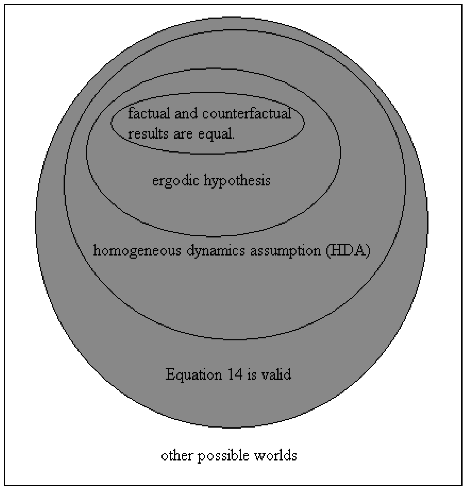
On the other hand, the ergodic hypothesis means that the time averages are equal to the ensemble average. As the latter is unique, it implies that all the time averages (both factual and counterfactual) are equal. Therefore, ergodicity ⇒ HDA. Yet, the HDA is different from ergodicity, for it is conceivable that the factual and the counterfactual time averages are equal among them, but that they are still different from the ensemble average. It is also conceivable that Equation (14) holds even if the HDA is not valid. The three counterfactual integrals in Equations (10) and (11) may all be different from each other, and still their sum may be equal to thrice the factual one. These different logical implications involved are summarized in Figure 2. The set of hypotheses painted in gray retrieve the usual meaning of Bell’s inequalities. In the “other possible worlds” (outside the gray set), there is no logical link between the observed violation of Bell’s inequalities and the validity of LR.
As can be seen in Figure 2, the HDA does not define the only possible world where Bell’s inequalities are retrieved. Yet, I believe the HDA to be the most plausible one in physical terms. It indicates that the time average of a dynamical variable recorded during the interval [t1, t1 + T] (say, when the variable is being observed) is equal to the time average recorded during any other interval [t2, t2 + T] (say, when the variable is not being observed) provided, of course, that T is sufficiently long. The relationship between the validity of the HDA and of a Markovian underlying dynamics seems intuitive, and deserves to be examined in detail elsewhere.
In fact, the HDA seems so plausible that doubts were raised on the existence of a physical situation where it does not hold. In other words, there is no doubt that possible worlds can be defined to violate the HDA (see [11]); the question is whether some physically reasonable model exists that, as a consequence of its evolution, violates the HDA. It is desirable that such model also violates Bell’s inequalities, and that it does so for some (not all) values of its parameters. In this way, the model is useful to study the relationship between the validity of the HDA and that of Bell’s inequalities. In the next section, one such model is proposed.
3. A Simple Model That Violates the Additional Hypotheses
3.1. A Classical Mixture with Delay
The QM predictions for the state |ϕ+〉 can be reproduced, regardless of the position of the analyzer in Station B (see Figure 1) by a statistical mixture of photon pairs polarized parallel and orthogonal to the analyzer in Station A, or
ρα = ½ {|α〉〈α|A⊗|α〉〈α|B + |α⊥〉〈α⊥|A⊗|α⊥〉〈α⊥|B}
This state is classical; it is able to reproduce the QM predictions only because the value of α is known by the source of photons. In the general case that {a,b} are the setting angles of the analyzers and α can be equal to a or not, the probability of coincidence produced by ρα is
which is the sum of the probabilities for the pair passing the analyzers as x-polarized or as y-polarized photons. Note that α is no longer the angle setting at Station A but that it plays the role of a hidden variable. Let us assume now that α evolves in time according to the following equation:
where the function a(t) is externally defined: it is the randomly varying angle setting in Station A. The argument of α in the rhs of Equation (18) is delayed a time τ > L/c to take into account the time required by the information (on the value of the angle setting a) to cover the spatial spread of the setup. Hence, the evolution of α(t) holds to locality. This is a sort of “measurement dependence bounded by locality.” The value of α is always well defined, which allows the calculation of both factual and counterfactual values of E(a,b). The parameter Γ, whose value is unknown, measures the strength of the tracking force that makes α(t) to follow the values taken by a(t). The QM predictions are fully retrieved in the limit τ→0.
P++(a,b,α) = ½ {cos2(a − α) × cos2(b − α) + sin2(a − α) × sin2(b − α)}
dα(t)/dt = −(Γ/τ) × [α(t − τ) −a(t)]
Equation (18) is a delay differential equation. It evolves in a phase space of infinite dimensions. The general solutions are difficult to find. In the particular case where a(t) = constant ≠ α(t = 0), α(t) decays slowly to a (=constant) if Γ << 1. If Γ ≈ 1, α(t) decays to a with damped oscillations of period ≈4τ. If Γ ≥ π/2, the amplitude of the oscillations of α(t) increases exponentially [21]. Be aware that the model discussed in [21] is similar, but different, from the one proposed here.
3.2. The Static Case
Let us consider first the case where the angle settings are mostly static. If T >> τ and Γ is not too small, then α(t) = a(t) during most of the time, the QM predictions are reproduced and SCHSH ≈ 2√2. One of the three counterfactual terms (the one with the actual value of a) in the rhs of Equations (10) and (11) is equal to the factual time average, and the other two terms are zero. To reproduce these results, note that P++ + P+− = ½ and P++ = P−−, so E(a,b,α) = 4 × P++(a,b,α) − 1, and use Equation (17). Hence, E(a,b) = E(a,b) = ±√2/2. Equation (14) is thus not fulfilled, and the usual CHSH inequality (Equation (1)) is not retrieved from Equation (13). In consequence, if values of measured E(a,b) are inserted into Equation (1), SCHSH > 2 (as was said before), but this result does not refute LR (because Equation (14) is not valid, so we are outside the gray set in Figure 2).
It is convenient defining a parameter Δ to quantify the violation of Equation (14):
where i,j here are the four usual setting angles {0,π/8,π/4,3π/8}. If Equation (14) holds, Δ = 0. In the static case discussed in this section, Δ = 2. The usual significance of the CHSH inequality is retrieved iff Δ = 0.
3.3. The Random Variable Case
The case when the angle settings are varied randomly, as in the experiments described in [3,7,8,9,10], is of special interest. A numerical simulation of Equation (18) is carried out, with a(t) jumping randomly, with a transition time equal to zero, between the values 0 and π/4. The jump times are also chosen randomly, at an average rate μ. The factual and the counterfactual time averages are computed. Each value of SCHSH and Δ is obtained after 2000τ with a coincidence rate of 500/τ and after discarding a transient of 200τ (total number of coincidences = 106). The initial condition for a(t < 0) = 0. The rate of incident pairs is high enough to follow the variations of α(t) in detail; be aware that this condition is far from having been reached in any experiment. Due to fluctuations caused by the randomness of the jumps, the strict equality Δ = 0 is never obtained numerically. In what follows, I will say that Equation (14) holds (then we are inside the gray set in Figure 2) if Δ <<1 (Δ ≈ 0), and that it is violated (then we are outside the gray set) if Δ ≈ 1.
For some parameters’ values, SCHSH > 2. In these cases, it is always found that Δ ≈ 1, that is, all the additional hypotheses are violated too. The inverse is not true: it is possible that Δ ≈ 1 and yet SCHSH < 2. In other words, the violation of the additional hypotheses is a condition necessary, but not sufficient, to retrieve the usual significance of Bell’s inequalities.
For example, in Figure 3, the variations of SCHSH and Δ as a function of the unknown parameter Γ are plotted for μτ = ¼. The vertical dotted lines at Γ ≈ 0.2 and Γ ≈ π/2 are the limits of the region where the CHSH inequality is violated. Note that, within this region, Δ ≥ 1. For Γ < 0.2, one gets SCHSH < 2, but it is still Δ ≈ 1. For Γ→0, Δ→0, and SCHSH→√2, which is the value produced by ρα if there is no correlation between α(t) and a(t). At Γ ≈ π/2, SCHSH falls to √2 and Δ to zero abruptly. The origin of these results is understood from the inspection of the behavior of α(t), see Figure 4. For Γ = 1 (Figure 4a) α(t) rapidly adjusts to the changing values of a(t), the condition α(t) ≈ a(t) holds most of the time and hence SCHSH > 2. For Γ = 0.1 (Figure 4b) α(t) follows a(t) too slowly. It reaches the target values 0 and π/4 only rarely and, in consequence, SCHSH < 2. The fact that Δ ≈ 1 in these two cases is a non-trivial result. For Γ = 0.02 (Figure 4c), the tracking force is too weak, and α(t) makes a low amplitude zigzag around the middle value π/8. Therefore, α(t) and a(t) are mostly uncorrelated and SCHSH ≈ √2. As α(t) is nearly constant, Equation (14) holds and Δ ≈ 0. If Γ ≥ π/2 (Γ = 2, Figure 4d) α(t) diverges exponentially, rotating faster and faster. The random jumps of a(t) make the evolution even wilder, reversing the rotation at random times. In consequence, α(t) loses any correlation with a(t). This explains why SCHSH falls abruptly to √2 at Γ ≈ π/2. The trajectory of α(t) in this case explores the whole phase space, apparently fulfilling the condition of “mixing” that makes the ergodic hypothesis valid. Thus, it is not surprising that Δ falls to zero abruptly at this point: ergodicity holds, so we are inside the gray set in Figure 2.
4. Summary and Discussion
The results of the measurements cannot be put into Bell’s inequality keeping its usual significance, unless at least one assumption in addition to LR is made. This additional assumption is the definition of a “possible world” to calculate the numerical values of the counterfactual terms in the inequality that is deduced assuming LR only (Equation (13)). The HDA is a possible world that assumes the equality between the time averages of factual and counterfactual expectation values. It is one of several possible worlds that retrieve the usual significance of Bell’s inequalities. Yet, there is no fundamental reason why these possible worlds must be valid in the setup of Figure 1. It is then possible to speculate that the experiments (reporting the violation of Bell’s inequalities) refuted the validity of these possible worlds (see Figure 2) and not of LR. The model in Section 3 assumes that the source in Figure 1 emits a mixture of photons polarized parallel and perpendicular to some angle α(t), and that α(t) tries to follow the variations of the angle set a in Station A, after a delay L/c and with a tracking force of strength Γ. This model holds to LR and, for some parameters’ values, it violates the possible worlds (or hypotheses) that allow retrieving the usual significance of Bell’s inequalities. I stress that it is not able (nor is intended) to reproduce the results of the recent loophole-free experiments, where μτ> 1. The model is devised only to explore the relationship between the violation of Equation (14) and usual Bell’s inequalities. It leads to the non-trivial result that the violation of Equation (14) is a condition necessary, but not sufficient, to violate Bell’s inequalities without violating LR.
As has been said, the impossibility of measuring with two settings at the same time is the cause of the necessity of an additional hypothesis. During the process of the revision of this paper, some reviewers proposed ingenious setups to circumvent this impossibility. However, no matter the ingenuity of the setup, at the end of the day the observer has to put each “click” (each photon detection, which occurs at a definite value of time) into one “box” (a box whose labels are defined by the setting that was used at that value of time). It is impossible, no matter the setup or the inequality used, to go back in time and observe where the click goes with a different setting. All of Bell’s inequalities involve well-defined numbers of clicks in boxes with well-defined and different labels. Recall that all measurements occur in the classical realm.
Bell’s inequalities are derived by integration over the ensemble of states of the hidden variables, which is a single integral. However, in the experiment, the numbers of clicks in each box are determined by separate time integrals that are, in principle, different from the single integral just mentioned. Therefore, the numbers of clicks in the boxes cannot be meaningfully inserted into the inequality. The two integrals are simply different unless it is assumed, for example, that the numbers of clicks in a given box depends only on the duration of the time lapse the corresponding setting is used (this is, roughly speaking, the HDA). As has been stated several times, this (or others alike) is an assumption in addition to LR. If no assumption in addition to LR is made, then only Equation (13) is valid. Moreover, Equation (13) includes counterfactual terms of unknown numerical value.
If the violation of Equation (14) were experimentally confirmed, it would be possible to reconcile QM with LR in spite of the observed violation of Bell’s inequalities. In Figure 4, the violation of Equation (14) is related with oscillations with a period of the order of L/c. In order to reveal these oscillations, an experiment should be able to follow the time evolution of the system (note that almost all performed experiments recorded only averaged values) with a resolution of at least L/2c. In all performed experiments, the rate of coincidences is orders of magnitude below this goal. Yet, a “stroboscopic” observation, which would sum up the results of many pulsed measurements, as it was done in [4], is at hand [22]. It must be warned that, if Equation (14) were actually violated in nature, the underlying real physical process would be presumably very different from the simple model presented in Section 3. The interesting question at this point is: How does one demonstrate from the experimental data whether Equation (14) is violated or not, given that the underlying physical process is unknown? If the model here presented is, to some extent at least, representative of the general case, a clue may be found again in the time behavior. Note that a α(t) “too simple” (like Γ << 1, Figure 4c), and one “too complex” (like Γ ≥ π/2, Figure 4d), both hold to Equation (14). It seems that Equation (14) is violated if the system has “complex, but not too complex,” behavior. Therefore, the degree of complexity of a time series may be a general way to reveal whether Equation (14) is violated, even if oscillations at ≈ L/c are not detected. This way is far from being easy: a practically computable definition of complexity is a controversial and difficult issue. Last but not least, the variables playing the role of α(t) are unknown and, perhaps, inaccessible in a direct way.
In spite of all these difficulties, I believe that time resolved measurements (as opposed to standard measurement of time averaged magnitudes) may offer a promising way out from the old QM vs. LR controversy. At least, now that the “loophole road” seems to be closed, they are something new to measure. If the violation of Equation (14) was actually observed, the resultant solution of the controversy might look like this: QM (as we know it) would be the steady state approximation (therefore, ergodicity holds) of a still unknown (and non-ergodic) LR theory underlying. This solution would be then similar to the old “statistical interpretation” of QM, enriched with non-ergodic evolution and dynamical complexity as its essential ingredients.
Acknowledgments
This work received support from the grant PIP CONICET 2011-01-077.
Conflicts of Interest
The author declares no conflict of interest.
References
- Clauser, J.; Shimony, A. Bell’s theorem: Experimental tests and implications. Rep. Prog. Phys. 1978, 41, 1881. [Google Scholar] [CrossRef]
- Aspect, A.; Dalibard, J.; Roger, G. Experimental test of Bell’s inequalities using time-varying analyzers. Phys. Rev. Lett. 1982, 49, 1804–1807. [Google Scholar] [CrossRef]
- Weihs, G.; Jennewein, T.; Simon, C.; Weinfurter, H.; Zeilinger, A. Violation of Bell’s inequality under strict Einstein locality conditions. Phys. Rev. Lett. 1998, 81, 5039–5043. [Google Scholar] [CrossRef]
- Agüero, M.; Hnilo, A.; Kovalsky, M. Time-resolved measurement of Bell’s inequalities and the coincidence loophole. Phys. Rev. A 2012, 86, 052121. [Google Scholar] [CrossRef]
- Giustina, M.; Mech, A.; Ramelow, S.; Wittmann, B.; Kofler, J.; Beyer, J.; Lita, A.; Calkins, B.; Gerrits, T.; Nam, S.; et al. Bell violation using entangled photons without the fair-sampling assumption. Nature 2013, 497, 227–230. [Google Scholar] [CrossRef] [PubMed]
- Christensen, B.; McCusker, K.T.; Altepeter, J.B.; Calkins, B.; Gerrits, T.; Lita, A.E.; Miller, A.; Shalm, L.K.; Zhang, Y.; Nam, S.W.; et al. Detection-Loophole-Free Test of Quantum Nonlocality, and Applications. Phys. Rev. Lett. 2013, 111, 130406. [Google Scholar] [CrossRef] [PubMed]
- Giustina, M.; Versteegh, M.A.M.; Wengerowsky, S.; Handsteiner, J.; Hochrainer, A.; Phelan, K.; Steinlechner, F.; Kofler, J.; Larsson, J.A.; Abellan, C.; et al. A Significant Loophole-Free Test of Bell’s Theorem with Entangled Photons. Phys. Rev. Lett. 2015, 115, 250401. [Google Scholar] [CrossRef] [PubMed]
- Shalm, L.; Meyer-Scott, E.; Christensen, B.G.; Bierhorst, P.; Wayne, M.A.; Stevens, M.J.; Gerrits, T.; Glancy, S.; Hamel, D.R.; Allman, M.S.; et al. A Strong Loophole-Free Test of Local Realism. Phys. Rev. Lett. 2015, 115, 250402. [Google Scholar] [CrossRef] [PubMed]
- Hensen, B.; Bernien, H.; Dr´eau, A.E.; Reiserer, A.; Kalb, N.; Blok, M.S.; Ruitenberg, J.; Vermeulen, R.F.L.; Schouten, R.N.; Abellán, C.; et al. Loophole-free Bell inequality violation using electron spins separated by 1.3 kilometres. Nature 2015, 526, 682–686. [Google Scholar] [CrossRef] [PubMed]
- Rosenfeld, W.; Burchardt, D.; Garthoff, R.; Redeker, K.; Ortegel, N.; Rau, M.; Weinfurter, H. Event-ready Bell-test using entangled atoms simultaneously closing detection and locality loopholes. arXiv, 2016; arXiv:1611.04604. [Google Scholar]
- Hnilo, A. Time weakens the Bell’s inequalities. arXiv, 2013; arXiv:quant-ph/1306.1383v2. [Google Scholar]
- Hnilo, A. Consequences of recent loophole-free experiments on a relaxation of measurement independence. Phys. Rev. A 2017, 95, 022102. [Google Scholar] [CrossRef]
- Buonomano, V. A limitation on Bell’s inequality. Ann. De L’I.H.P. 1978, 29, 379–394. [Google Scholar]
- Khrennikov, A. Interpretations of Probability; Walter de Gruyter: Berlin, Germany, 2009. [Google Scholar]
- De Muynck, W. Foundations of Quantum Mechanics, An Empiricist Approach; Kluwer: Boston, MA, USA, 2002. [Google Scholar]
- Notarrigo, S. A Newtonian separable model which violates Bell’s inequality. Nuova Cim. 1984, 83, 173–187. [Google Scholar] [CrossRef]
- Larsson, J.; Gill, R. Bell’s inequality and the coincidence-time loophole. Europhys. Lett. 2004, 67, 707–713. [Google Scholar] [CrossRef]
- D’Espagnat, B. Nonseparability and the tentative descriptions of reality. Phys. Rep. 1984, 110, 201–264. [Google Scholar] [CrossRef]
- Buchanan, M. Gamble with time. Nat. Phys. 2013, 9, 3. [Google Scholar] [CrossRef]
- Peters, O. The time resolution of the St.Petersburg paradox. Philos. Trans. R. Soc. A 2013, 369, 4913–4931. [Google Scholar] [CrossRef] [PubMed]
- Hnilo, A. Observable consequences of a hypothetical transient deviation from Quantum Mechanics. arXiv, 2012; arXiv:quant-ph/1212.5722v2. [Google Scholar]
- Agüero, M.; Hnilo, A.; Kovalsky, M. Measuring the entanglement of photons produced by a nanosecond pulsed source. J. Opt. Soc. Am. B 2014, 31, 3088–3096. [Google Scholar] [CrossRef]
Figure 1.
Scheme of a typical experiment to test Bell’s inequalities. The source S emits pairs of photons entangled in polarization towards Stations A and B separated by a distance L. At each station, the analyzer is set at some angle value. The expectation value E(α,β) is measured from the number of coincidences at each pair of outputs, recorded during some time interval (which can be continuous, or not). A photon detected in the transmitted (reflected) output of the analyzers is defined as a + (−) result.
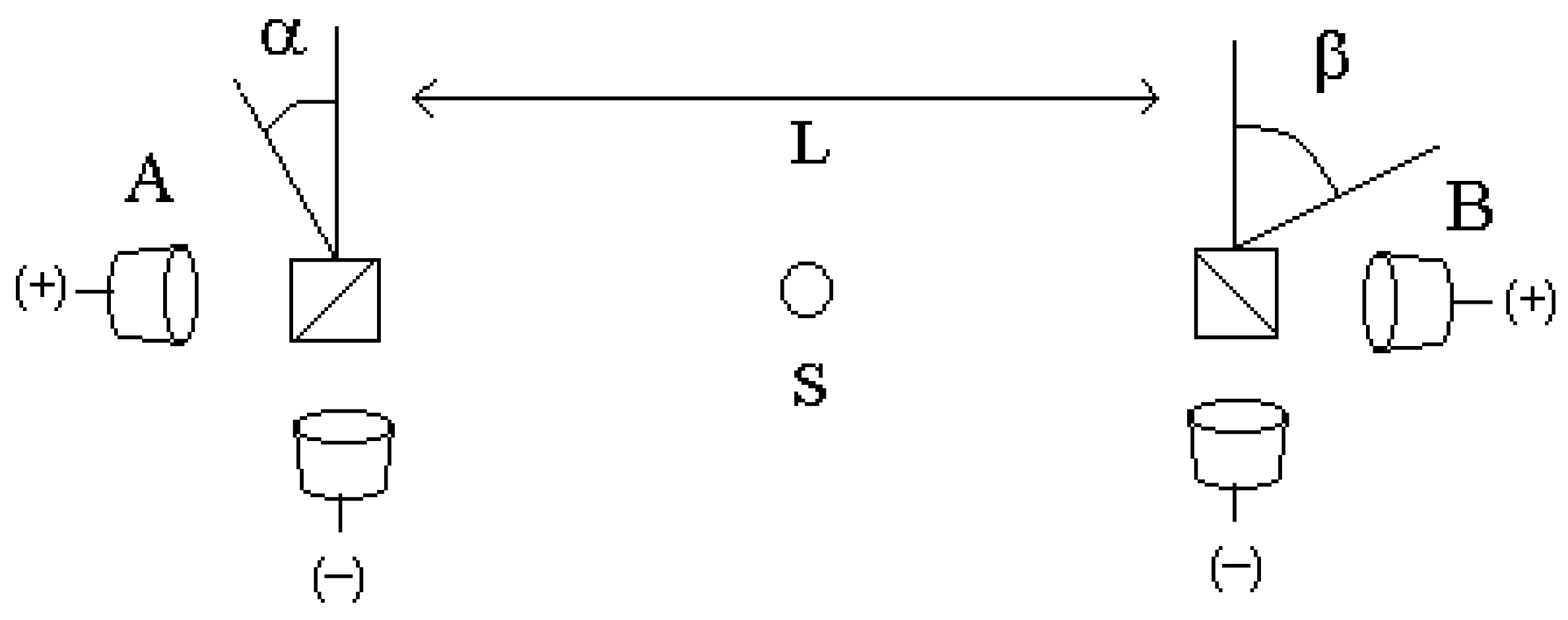
Figure 2.
Logical relationship between different additional hypotheses defining different “possible worlds.” For example, in a possible world where the ergodic hypothesis is valid, the homogeneous dynamics assumption (HDA)and Equation (14) are also valid. In this same possible world, the equality between factual and counterfactual results may be valid or not. The hypotheses in gray retrieve the usual significance of Bell’s inequalities. In the “other possible worlds” (some of them are discussed in [11]), there is no logical link between the observed violation of Bell’s inequalities and the validity of local realism (LR).

Figure 3.
SCHSH and Δ as a function of Γ, μτ = ¼. The horizontal dotted line indicates the CHSH bound.
Figure 3.
SCHSH and Δ as a function of Γ, μτ = ¼. The horizontal dotted line indicates the CHSH bound.
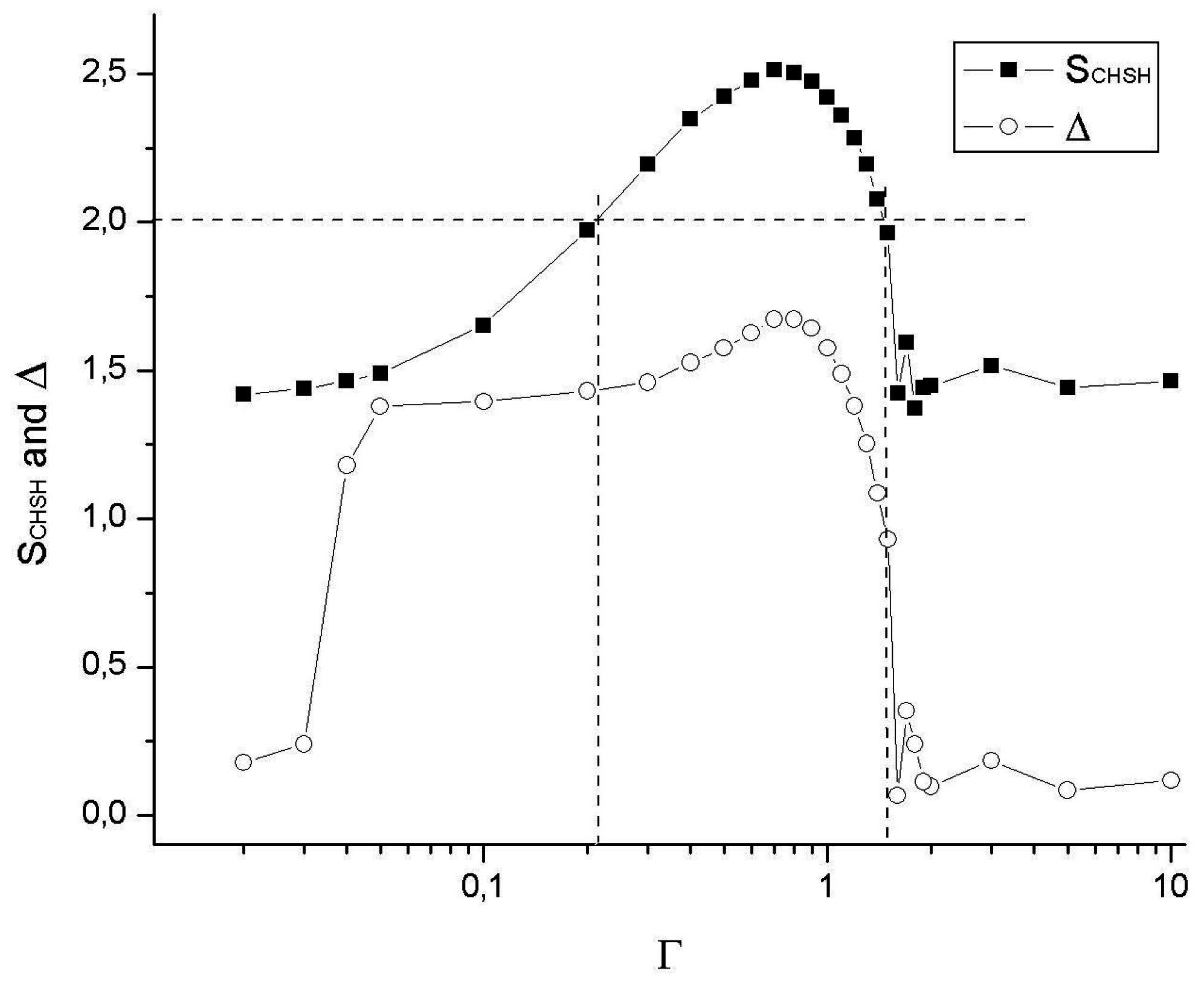
Figure 4.
Evolution of the hidden variable α(t) for μτ = ¼ and several values of Γ, note the different vertical scales; (a) for Γ = 1, α(t) promptly follows the random jumps of a(t) between 0 and π/4, SCHSH > 2 and Δ ≈ 1; (b) for Γ = 0.1, α(t) follows a(t) slowly, rarely reaching 0 or π/4, Δ ≈ 1 but SCHSH < 2; (c) for Γ = 0.02, α(t) zigzags around π/8 never reaching 0 or π/4, SCHSH ≈ √2 and Δ ≈ 0; (d) for Γ = 2, α(t) varies wildly, filling the whole phase space and losing correlation with a(t), SCHSH ≈ √2 and Δ ≈ 0.

© 2017 by the author. Licensee MDPI, Basel, Switzerland. This article is an open access article distributed under the terms and conditions of the Creative Commons Attribution (CC BY) license (http://creativecommons.org/licenses/by/4.0/).
Share and Cite
MDPI and ACS Style
Hnilo, A.A. Using Measured Values in Bell’s Inequalities Entails at Least One Hypothesis in Addition to Local Realism. Entropy 2017, 19, 180. https://doi.org/10.3390/e19040180
AMA Style
Hnilo AA. Using Measured Values in Bell’s Inequalities Entails at Least One Hypothesis in Addition to Local Realism. Entropy. 2017; 19(4):180. https://doi.org/10.3390/e19040180
Chicago/Turabian StyleHnilo, Alejandro Andrés. 2017. "Using Measured Values in Bell’s Inequalities Entails at Least One Hypothesis in Addition to Local Realism" Entropy 19, no. 4: 180. https://doi.org/10.3390/e19040180
Note that from the first issue of 2016, this journal uses article numbers instead of page numbers. See further details here.