Article

The Solution of Modified Fractional Bergman’s Minimal Blood Glucose-Insulin Model

1
Mathematics Department, College of Science, King Saud University, Riyadh 11989, Saudi Arabia
2
Department of Mathematics, Yagyavalkya Institute of Technology, Jaipur 302035, India
3
School of Liberal Studies, Ambedkar University Delhi, Delhi 110006, India
*
Author to whom correspondence should be addressed.
Entropy 2017, 19(5), 114; https://doi.org/10.3390/e19050114
Submission received: 21 January 2017 / Revised: 4 March 2017 / Accepted: 9 March 2017 / Published: 2 May 2017
(This article belongs to the Special Issue Wavelets, Fractals and Information Theory II)

Abstract

:
In the present paper, we use analytical techniques to solve fractional nonlinear differential equations systems that arise in Bergman’s minimal model, used to describe blood glucose and insulin metabolism, after intravenous tolerance testing. We also discuss the stability and uniqueness of the solution.

1. Introduction

Mathematical modeling is a very important branch of applied mathematics. By using this approach, we can convert a real world problem into a mathematical module and then analyze it in a better manner. In the 1990s when researchers were faced with the blood or blood’s constituent dynamical transport phenomena, they used classical theory to describe these processes [1,2,3]. After that, many researchers conducted research in that direction to remove the complexity of this phenomenon [1,2,3,4,5,6,7].
Regarding research modules , one of the most important modules is Bergman’s minimal model [4,5,6]. In this model, a body is described as a compartment with a basal concentration of glucose and insulin. Bergman’s minimal model has two variations. the first describes glucose kinetics, and the second describes insulin kinetics. The two models have mostly been used to understand the kinetics during IVGTT test (Glucose Tolerance Test) [7,8].
In applied mathematics, one of the most used concepts is the derivative. Derivatives show the rate of change of a function. This is helpful to describe many real phenomena. After this research, mathematicians faced some complex problems of the real world; to solve them, mathematicians introduced the fractional derivative [9,10,11,12,13]. The concept of fractional calculus has great importance in many branches and is also important for modeling real world problems [14,15,16,17].
For this reason, many researchers have engaged in a great amount of research work, conferences, and paper publications. Various definitions of fractional derivatives have been given to date. Recently, researchers have described a new fractional derivative operator named the Caputo–Fabrizio fractional derivative [18,19,20,21]. In this paper, we use this operator to describe the Bergman’s minimal glucose-insulin model and solve it by the iterative technique.

2. The Caputo–Fabrizio Fractional Order Derivative

Singularity at the end point of the interval is the main problem that is faced with the definition of the fractional order derivative. To avoid this problem, Caputo and Fabrizio recently proposed a new fractional order derivative that does not have any singularity. The novel fractional derivative given by Caputo and Fabrizio is more suitable to describe the rate of change in concentration of the model because its kernel is non-local and non-singular. The definition is based on the convolution of a first-order derivative and the exponential function, given in the following definition:
Definition 1.
Let f H 1 ( a , b ) , b > a , α [ 0 , 1 ] . Then, the new fractional order Caputo derivative is defined as:
D t α f ( t ) = M ( α ) 1 α a t f x e α t x 1 α dx .
Here M ( α ) denotes the normalization function such that M ( 0 ) = M ( 1 ) = 1 ; for detail, see [18]. If the function does not belong to H 1 ( a , b ) , then the derivative can be written as
D t α f ( t ) = α M ( α ) 1 α a t f t f x e α t x 1 α dx .
Remark 1.
The authors state that if σ = 1 α α [ 0 , ) , α = 1 1 + σ [ 0 , 1 ] , then Equation (2) reduces to
D t α f ( t ) = N ( σ ) σ a t f x e t x σ dx , N ( 0 ) = N ( ) = 1
and
lim σ 0 1 σ e t x 1 α = δ ( x t ) .
As we have defined a new derivative above, then there should be its anti-derivative; the integral of this new fractional derivative is given by Losada and Nieto [19].
Definition 2.
The fractional integral of order α 0 < α < 1 of the function f is defined below:
I α t f ( t ) = 2 1 α 2 α M α f t + 2 α 2 α M α 0 t f ( s ) d s , t 0 .
Remark 2.
It is clear from Equation (5) that the fractional integral of order α 0 < α < 1 is an average of function f and its integral of order 1. Hence we get the condition [19]:
2 1 α 2 α M α + 2 α 2 α M α = 1 ,
the above term yields an explicit formula,
M α = 2 2 α , 0 < α < 1 .
Due to the above relation, Nieto and Losada [19] anticipated that the new Caputo derivative of order 0 < α < 1 could be written as:
0 C F D t α f ( t ) = 1 1 α a t f x e α t x 1 α dx .
Theorem 1.
Here f ( t ) denotes the normalization function such as
f s ( a ) = 0 , s = 1 , 2 , , n
then, we have
D t α D t n f t = D t n D t α f t
For more detail see [18,19].

3. Bergman’s Minimal Model Fractional Module

The minimal model of the glucose insulin kinetics has been proposed to describe the time course of these concentrations. We will use the standard formulation of the minimal model represented by the following system of differential equations:
0 C F D t α G ( t ) = p 1 + X ( t ) G ( t ) + p 1 G b , 0 < α < 1 0 C F D t β X ( t ) = p 2 X ( t ) + p 3 I ( t ) I b , 0 < β < 1 0 C F D t γ I ( t ) = p 6 G ( t ) p 5 + t p 4 I ( t ) I b , 0 < γ < 1
subject to initial conditions,
G 0 = G 0 , X 0 = X 0 , I 0 = I 0
The parameters for the minimal model (11) are given in Table 1.
This model can be used to describe the pancreas as the source of insulin. In a healthy individual, a small amount of insulin is always created and cleared [4]. This helps to keep the basal concentration I b . The glucose-independent production and clearance of insulin is proportional to the blood insulin concentration. If the insulin level is above basal concentration, clearance increases. On the other hand, if the insulin level is below basal concentration, production increases. When the glucose level gets high, the pancreas reacts by releasing more insulin at a given rate. To explain this mathematically, one has to derive a function describing the reaction of the pancreas. This function was derived by Bergman et al. and adjusted by Gaetano et al. [7,8] to become Pancreas(t) = G ( t ) p 5 + t , where G ( t ) p 5 + = max ( G ( t ) p 5 , 0).

4. Existence of the Coupled Solutions

By using the Fixed-Point theorem, we define the existence of the solution. First, transform Equation (11) into an integral equation as follows:
G t G 0 = 0 C F I t α p 1 + X ( t ) G ( t ) + p 1 G b ,
X ( t ) X 0 = 0 C F I t β p 2 X ( t ) + p 3 I ( t ) I b ,
I ( t ) I ( 0 ) = 0 C F I t β p 6 G ( t ) p 5 + t p 4 I ( t ) I b ,
on using the definition defined by Nieto, we get
G t = G 0 + 2 ( 1 α ) ( 2 α ) M ( α ) p 1 + X ( t ) G ( t ) + p 1 G b + 2 α ( 2 α ) M ( α ) 0 t p 1 + X ( s ) G ( s ) + p 1 G b d s ,
and
X ( t ) = X 0 + 2 ( 1 β ) ( 2 β ) M ( β ) p 2 X ( t ) + p 3 I ( t ) I b + 2 β ( 2 β ) M ( β ) 0 t p 2 X ( s ) + p 3 I ( s ) I b d s ,
we also have
I ( t ) = I 0 + 2 ( 1 γ ) ( 2 γ ) M ( γ ) p 6 G ( t ) p 5 + t p 4 I ( t ) I b + 2 γ ( 2 γ ) M ( γ ) 0 t p 6 G ( s ) p 5 + t p 4 I ( s ) I b d s .
Let us consider the following kernels:
K 1 ( t , G ) = p 1 + X ( t ) G ( t ) + p 1 G b ,
K 2 ( t , X ) = p 2 X ( t ) + p 3 I ( t ) I b ,
K 3 ( t , I ) = p 6 G ( t ) p 5 + t p 4 I ( t ) I b .
Theorem 2.
Show that K 1 , K 2 , and K 3 satisfy Lipschiz condition.
Proof. 
First we prove this condition for K 1 . Let G and G 1 be two functions, then we have
K 1 ( t , G ) K 1 ( t , G 1 ) = p 1 + X ( t ) G t p 1 + X ( t ) G 1 t ,
on using the Cauchy’s inequality, we get
K 1 ( t , G ) K 1 ( t , G 1 ) p 1 + X ( t ) G t G 1 t ,
or
K 1 ( t , G ) K 1 ( t , G 1 ) H G t G 1 t ,
where
p 1 + X ( t ) H .
Additionally, for K 2 ,
K 2 ( t , X ) K 2 ( t , X 1 ) = p 2 X ( t ) + p 3 I t I b p 2 X 1 ( t ) + p 3 I t I b ,
on using the Cauchy’s inequality, we get
K 2 ( t , X ) K 2 ( t , X 1 ) p 2 X t X 1 t ,
or
K 2 ( t , X ) K 2 ( t , X 1 ) H 1 X t X 1 t ,
where
p 2 H 1 .
Similarly, for K 3 ,
K 3 ( t , I ) K 3 ( t , I 1 ) = p 6 G ( t ) p 5 + t p 4 I t I b p 6 G ( t ) p 5 + t p 4 I 1 t I b ,
by Cauchy’s inequality
K 3 ( t , I ) K 3 ( t , I 1 ) p 4 I t I 1 t ,
or
K 3 ( t , I ) K 3 ( t , I 1 ) H 2 I t I 1 t ,
where
p 4 H 2 .
We consider the following recursive formula
G n t = 2 ( 1 α ) ( 2 α ) M α K 1 ( t , G n 1 ) + 2 α ( 2 α ) M α 0 t K 1 ( s , G n 1 ) d s ,
and
X n t = 2 ( 1 β ) ( 2 β ) M β K 2 ( t , X n 1 ) + 2 β ( 2 β ) M β 0 t K 2 ( s , X n 1 ) d s ,
as well as
I n t = 2 ( 1 γ ) ( 2 γ ) M γ K 3 ( t , I n 1 ) + 2 γ ( 2 γ ) M γ 0 t K 3 ( s , I n 1 ) d s .
Now the difference between the consecutive terms is
U n t = G n t G n 1 t = 2 ( 1 α ) ( 2 α ) M α K 1 ( t , G n 1 ) 2 ( 1 α ) ( 2 γ ) M α K 1 ( t , G n 2 ) + 2 α ( 2 γ ) M α 0 t K 1 ( s , G n 1 ) K 1 ( s , G n 1 ) d s ,
V n t = X n t X n 1 t = 2 ( 1 β ) ( 2 β ) M β K 2 ( t , X n 1 ) 2 ( 1 β ) ( 2 β ) M β K 2 ( t , X n 1 ) + 2 β ( 2 β ) M β 0 t K 2 ( s , X n 1 ) K 2 ( s , X n 1 ) d s ,
and
W n t = I n t I n 1 t = 2 ( 1 γ ) ( 2 γ ) M γ K 3 ( t , I n 1 ) 2 ( 1 γ ) ( 2 γ ) M γ K 3 ( t , I n 1 ) + 2 γ ( 2 γ ) M γ 0 t K 3 ( s , I n 1 ) K 3 ( s , I n 2 ) d s .
It is worth noting that
G n t = i = 0 U i t , X n t = i = 0 V i t , I n t = i = 0 W i t .
Now take norm on both sides of Equations (37)–(39), respectively
U n t = G n t G n 1 t = 2 ( 1 α ) ( 2 α ) M α K 1 ( t , G n 1 ) 2 ( 1 α ) ( 2 α ) M α K 1 ( t , G n 2 ) + 2 α ( 2 α ) M α 0 t K 1 ( s , G n 1 ) K 1 ( s , G n 2 ) d s ,
and
V n t = X n t X n 1 t = 2 ( 1 α ) ( 2 β ) M β K 2 ( t , X n 1 ) 2 ( 1 β ) ( 2 β ) M β K 2 ( t , X n 2 ) + 2 β ( 2 β ) M β 0 t K 2 ( s , X n 1 ) K 2 ( s , X n 2 ) d s ,
as well as
W n t = I n t I n 1 t = 2 ( 1 γ ) ( 2 γ ) M γ K 3 ( t , I n 1 ) 2 ( 1 γ ) ( 2 γ ) M γ K 3 ( t , I n 2 ) + 2 γ ( 2 γ ) M γ 0 t K 3 ( s , I n 1 ) K 3 ( s , I n 2 ) d s .
From Equations (40)–(42), by using triangular inequality
U n t = G n t G n 1 t 2 ( 1 α ) ( 2 α ) M α K 1 ( t , G n 1 ) K 1 ( t , G n 2 ) + 2 α ( 2 α ) M α 0 t K 1 ( s , G n 1 ) K 1 ( s , G n 2 ) d s ,
V n t = X n t X n 1 t = 2 ( 1 β ) ( 2 β ) M β K 2 ( t , X n 1 ) K 2 ( t , X n 2 ) + 2 β ( 2 β ) M β 0 t K 2 ( s , X n 1 ) K 2 ( s , X n 2 ) d s ,
and
W n t = I n t I n 1 t = 2 ( 1 γ ) ( 2 γ ) M γ K 3 ( t , I n 1 ) K 3 ( t , I n 2 ) + 2 γ ( 2 γ ) M γ 0 t K 3 ( s , I n 1 ) K 3 ( s , I n 2 ) d s .
Since the kernel satisfies the Lipchitz condition, we obtain:
U n t = G n t G n 1 t 2 ( 1 α ) ( 2 α ) M α H G n 1 G n 2 + 2 α ( 2 α ) M α K 0 t G n 1 G n 2 d s ,
V n t = X n t X n 1 t 2 ( 1 β ) ( 2 β ) M β H 1 X n 1 X n 2 + 2 β ( 2 β ) M β J 1 0 t X n 1 X n 2 d s ,
W n t = I n t I n 1 t 2 ( 1 γ ) ( 2 γ ) M γ H 2 I n 1 I n 2 + 2 γ ( 2 γ ) M γ J 2 0 t I n 1 I n 2 d s .
Theorem 3.
Show that the Bergman’s Minimal Model Fractional Module is the minimal model of the glucose insulin kinetics having a solution.
Proof. 
As we have seen that the above Equations (43)–(45) are bounded, and we have proven that the kernels satisfy Lipschiz condition, therefore following the results obtained in Equations (43)–(45) using the recursive technique, we get the following relation
U n t G 0 + 2 ( 1 α ) ( 2 α ) M α H n + 2 α ( 2 α ) M α K t n ,
and
V n t X 0 + 2 ( 1 β ) ( 2 β ) M β H 1 n + 2 β ( 2 β ) M β J 1 t n ,
as well as
W n t I 0 + 2 ( 1 γ ) ( 2 γ ) M γ H 2 n + 2 γ ( 2 γ ) M γ J 2 t n .
Therefore, the above solutions exist and are continuous. Nonetheless, to show that the above is a solution of Equation (11), we get
G t = G n t P n t X t = X n t Q n t I t = I n t R n t ,
where P n , Q n and R n are remainder terms of series solution. Thus,
G t G n t = 2 ( 1 α ) ( 2 γ ) M α K 1 t , G P n t + 2 α ( 2 α ) M α 0 t K 1 s , G P n s d s ,
and
X t X n t = 2 ( 1 β ) ( 2 β ) M β K 2 t , X Q n t + 2 β ( 2 β ) M β 0 t K 2 s , X Q n s d s ,
as well as
I t I n t = 2 ( 1 γ ) ( 2 γ ) M γ K 3 t , I R n t + 2 γ ( 2 γ ) M γ 0 t K 3 s , I R n s d s .
It follows from the above that:
G t 2 ( 1 α ) ( 2 α ) M α K 1 ( t , G ) G 0 2 α ( 2 α ) M α 0 t K 1 ( s , G ) d s = P n t + 2 ( 1 α ) ( 2 α ) M α K 1 ( t , G ) + 2 α ( 2 α ) M α 0 t K 1 s , G P n t K 1 s , G d s .
Now, applying the norm on both sides and using the Lipchitz condition, we get
G t 2 ( 1 α ) ( 2 α ) M α K 1 ( t , G ) G 0 2 α ( 2 α ) M α 0 t K 1 ( s , G ) d s P n t + 2 ( 1 α ) ( 2 α ) M α H + 2 α ( 2 α ) M α K t P n t ,
similarly, we get
X t 2 ( 1 β ) ( 2 β ) M β K 2 ( t , X ) X 0 2 β ( 2 β ) M β 0 t K 2 ( s , X ) d s Q n t + 2 ( 1 β ) ( 2 β ) M β H 1 + 2 β ( 2 β ) M β J 1 t Q n t ,
and
I t 2 ( 1 γ ) ( 2 γ ) M γ K 3 ( t , I ) I 0 2 γ ( 2 γ ) M γ 0 t K 3 ( s , I ) d s R n t + 2 ( 1 γ ) ( 2 γ ) M γ H 2 + 2 γ ( 2 γ ) M γ K 2 t R n t .
On taking the limit n of Equations (54)–(56), we get
G t = 2 ( 1 α ) ( 2 α ) M α K 1 ( t , G ) + G 0 + 2 α ( 2 α ) M α 0 t K 1 ( s , G ) d s ,
X t = 2 ( 1 β ) ( 2 β ) M β K 2 ( t , X ) + X 0 + 2 β ( 2 β ) M β 0 t K 2 ( s , X ) d s ,
and
I t = 2 ( 1 γ ) ( 2 γ ) M γ K 3 ( t , I ) + I 0 + 2 γ ( 2 γ ) M γ 0 t K 3 ( s , I ) d s .
Equations (57)–(59) is the solution of the system (11); therefore, we can say that a solution exists. ☐

Uniqueness of the Solutions

In this part, we want to show that solutions presented in the above section are unique.
To prove this, we can another solutions for system (11), say G t , X t , a n d I t ; then:
G t G 1 t = 2 ( 1 α ) ( 2 α ) M α K 1 ( t , G ) K 1 ( t , G 1 ) + 2 α ( 2 α ) M α 0 t K 1 ( s , G ) K 1 ( s , G 1 ) d s ,
apply the norm both sides of Equation (60),
G t G 1 t 2 ( 1 α ) ( 2 α ) M α K 1 ( t , G ) K 1 ( t , G 1 ) + 2 α ( 2 α ) M α 0 t K 1 ( s , G ) K 1 ( s , G 1 ) d s .
On using the Lipchitz condition, having the fact in mind that the solution is bounded, we get
G t G 1 t < 2 ( 1 α ) ( 2 α ) M α H D + 2 α ( 2 α ) M α J 1 D t n
this is true for any n; hence,
G t = G 1 t
Similarly, we get
X t = X 1 t
and
I t = I 1 t .
Hence, it shows the uniqueness of the solution of system (11).

5. Application of Caputo–Fabrizio Derivative to Bergman’s Minimal Model

Watugala introduced the Sumudu transform in early 1990s [20]. The Sumudu transform is defined over the set of functions:
A = { f ( t ) M , τ 1 , τ 2 > 0 , f ( t ) < M e t τ j , i f t ( 1 ) j × [ 0 , ) } ,
the Sumudu transform is defined by
G ˜ ( u ) = S T [ f ( t ) ] = 0 f ( u t ) e t d t , u ( τ 1 , τ 2 )
for detail, see [15,16,21].
Theorem 4.
Let f t be a function for which the Caputo–Fabrizio exists; then, the Sumudu transform of the Caputo–Frabrizio fractional derivative of f t is given as:
S T 0 C F D t α f ( t ) = M ( α ) S T f t f 0 1 α + α u .

Solution of Fractional Module by Sumudu Transform

Since the Bergman’s Minimal Model Fractional Module has three equations, it may be challenging to get the exact solution. To obtain the best solution, we will use an iterative technique with the help of the Sumudu Transform.
Applying the Sumudu transform on both sides of (11), we get
M ( α ) S T G t G 0 1 α + α u = S T p 1 + X ( t ) G ( t ) + p 1 G b ,
or
S T G t = G 0 + 1 α + α u M ( α ) S T p 1 + X ( t ) G ( t ) + p 1 G b .
Applying the inverse Sumudu transform on both sides of (67), we get
G t = G 0 + S T 1 1 α + α u M ( α ) S T p 1 + X ( t ) G ( t ) + p 1 G b ,
and in the same manner
X t = X 0 + S T 1 1 β + β u M ( β ) S T p 2 X ( t ) + p 3 I ( t ) I b ,
and
I t = I 0 + S T 1 1 γ + γ u M ( γ ) S T p 6 G ( t ) p 5 + t p 4 I ( t ) I b .
We next obtain the following recursive formula from (68)–(70):
G n + 1 t = G n 0 + S T 1 1 α + α u M ( α ) S T p 1 + X n ( t ) G n ( t ) + p 1 G b ,
X n + 1 t = X n 0 + S T 1 1 α + α u M ( α ) S T p 2 X n ( t ) + p 3 I n ( t ) I b ,
and
I n + 1 t = I n 0 + S T 1 1 α + α u M ( α ) S T p 6 G n ( t ) p 5 + t p 4 I n ( t ) I b .
The solution is thus provided as:
G ( t ) = lim n G n ( t )
X ( t ) = lim n X n ( t )
I ( t ) = lim n I n ( t )
we get the required solution.

6. Numerical Solution

As a particular instance to be treated, we assume the base level blood glucose concentration to be G b = 92 mg/dL, while the base level blood concentration of insulin to be I b = 7.3 mU/L. The glucose clearance rate independent of insulin is p 1 = 0.03082 min−1, the rate of clearance of active insulin (decrease of uptake) is p 2 = 0.02093 min−1, the increase in uptake ability caused by insulin is p 3 = 1.062 × 10 5 L/(min2·mU), the decay rate of blood insulin is p 4 = 0.3 min−1, the target glucose level is p 5 = 89.5 mg/dL, and the rate of pancreatic release after glucose bolus is p 6 = 0.3349 × 10 2 mUdL/L·mg·min. Substituting the above values in (74)–(76) with G 0 = 287 mg/DL, X 0 = 0 mg/DL, and I 0 = 403.4 mg/DL, the numerical solution is described by Figure 1.

7. Conclusions

This paper is an attempt to describe the existence and uniqueness of the Bergman Minimal Model which is extended by Caputo–Fabrizio fractional derivative in the context of glucose and insulin levels in blood. We obtain the approximate solution of the Model and a numerical solution of the system which shows that effect of time on the concentrations G ( t ) , X ( t ) , and I ( t ) .

Acknowledgments

The authors extend their sincere appropriations to the Deanship of Scientific Research at King Saud University for its funding this Profile Research Group (PRG-1437-35). Further authors are thankful to reviewers for giving their fruitful comments to improve this paper.

Author Contributions

All authors contributed equally in the paper. All authors have read and approved the final manuscript.

Conflicts of Interest

The authors declare no conflict of interest.

References

  1. Eckstein, E.C.; Belgacem, F.B.M. Model of platelet transport in flowing blood with drift and diffusion terms, extended platelet transport equation. Biophys. J. 1991, 60, 53–69. [Google Scholar] [CrossRef]
  2. Mountrakis, L.; Lorenz, E.; Hoekstra, A.G. Where do the platelets go? A simulation study of fully resolved blood flow through aneurysm vessels. Interface Focus 2013, 3, 1–10. [Google Scholar] [CrossRef] [PubMed]
  3. Bourouiba, L.; Dehandschoewercker, E.; Bush, J.W.M. Violent expiratory events: On coughing and sneezing. J. Fluid Mech. 2014, 745, 537–563. [Google Scholar] [CrossRef]
  4. Caumo, A.; Cobelli, C.; Omenetto, M. Overestimation of minimal model glucose effectiveness in presence of insulin response is due to under modeling. Am. J. Physiol. 1999, 278, 481–488. [Google Scholar]
  5. Bergman, R.N.; Ider, Y.Z.; Bowden, C.R.; Cobelli, C. Quantitative estimation of insulin sensitivity. Am. J. Physiol. 1979, 236, 667–677. [Google Scholar]
  6. Bowden, C.R.; Bergman, R.N.; Toffolo, G.; Cobelli, C. Minimal modeling, partition analysis, and identification of glucose disposal in animals and man. IEEE Trans. Biomed. Eng. 1980, 18, 129–135. [Google Scholar]
  7. Gaetano, A.D.; Arino, O. Mathematical modeling of the intravenous glucose tolerance test. J. Math. Biol. 2000, 40, 136–168. [Google Scholar] [CrossRef] [PubMed]
  8. Gatewood, L.C.; Ackerman, E.; Rosevear, J.W.; Molnar, G.D.; Burns, T.W. Tests of a mathematical model of the blood-glucose regulatory system. Comput. Biomed. Res. 1968, 2, 1–14. [Google Scholar] [CrossRef]
  9. Caputo, M. Linear models of dissipation whose Q is almost frequency independent, part II. Geophys. J. Int. 1967, 13, 529–539. [Google Scholar] [CrossRef]
  10. Podlubny, I. Fractional Differential Equations; Academic Press: New York, NY, USA, 1999. [Google Scholar]
  11. Kilbas, A.A.; Srivastava, H.M.; Trujillo, J.J. Theory and Applications of Fractional Differential Equations; Elsevier: Amsterdam, The Netherlands, 2006. [Google Scholar]
  12. Chaurasia, V.B.L.; Dubey, R.S. Analytical solution for the differential equation containing generalized fractional derivative operators and Mittag-Leffler-type function. ISRN Appl. Math. 2011, 2011, 682381. [Google Scholar] [CrossRef]
  13. Chaurasia, V.B.L.; Dubey, R.S. Analytical solution for the generalized time-fractional telegraph equation. Fract. Differ. Calc. 2013, 3, 21–29. [Google Scholar] [CrossRef]
  14. Atangana, A.; Alabaraoye, E. Solving a system of fractional partial differential equations arising in the model of HIV infection of CD4+ cells and attractor one-dimensional Keller-Segel equations. Adv. Differ. Equ. 2013, 2013, 94. [Google Scholar] [CrossRef]
  15. Chaurasia, V.B.L.; Dubey, R.S.; Belgacem, F.B.M. Fractional radial diffusion equation analytical solution via hankel and Sumudu transforms. Math. Eng. Sci. Aerosp. 2012, 3, 1–10. [Google Scholar]
  16. Dubey, R.S.; Goswami, P.; Belgacem, F.B.M. Generalized time-fractional telegraph equation analytical solution by Sumudu and Fourier transforms. J. Fract. Calc. Appl. 2014, 5, 52–58. [Google Scholar]
  17. Belgacem, F.B.M. Diffusion and drift models for population dispersal from stochastic and continuum views. Int. J. Appl. Math. 2001, 5, 85–106. [Google Scholar]
  18. Caputo, M.; Fabrizio, M. A new Definition of Fractional Derivative without Singular Kernel. Prog. Fract. Differ. Appl. 2015, 1, 73–85. [Google Scholar]
  19. Losada, J.; Nieto, J.J. Properties of a New Fractional Derivative without Singular Kernel. Fract. Differ. Appl. 2015, 1, 87–92. [Google Scholar]
  20. Atangana, A.; Alkahtani, B.S.T. Extension of the RLC electrical circuit to fractional derivative without singular kernel. Adv. Mech. Eng. 2015, 7, 1–6. [Google Scholar]
  21. Dubey, R.S.; Alkahtani, B.S.T.; Atangana, A. Analytical solution of space-time fractional Fokker–Plank equation by homotopy perturbation Sumudu transform method. Math. Probl. Eng. 2015, 2015, 780929. [Google Scholar] [CrossRef]
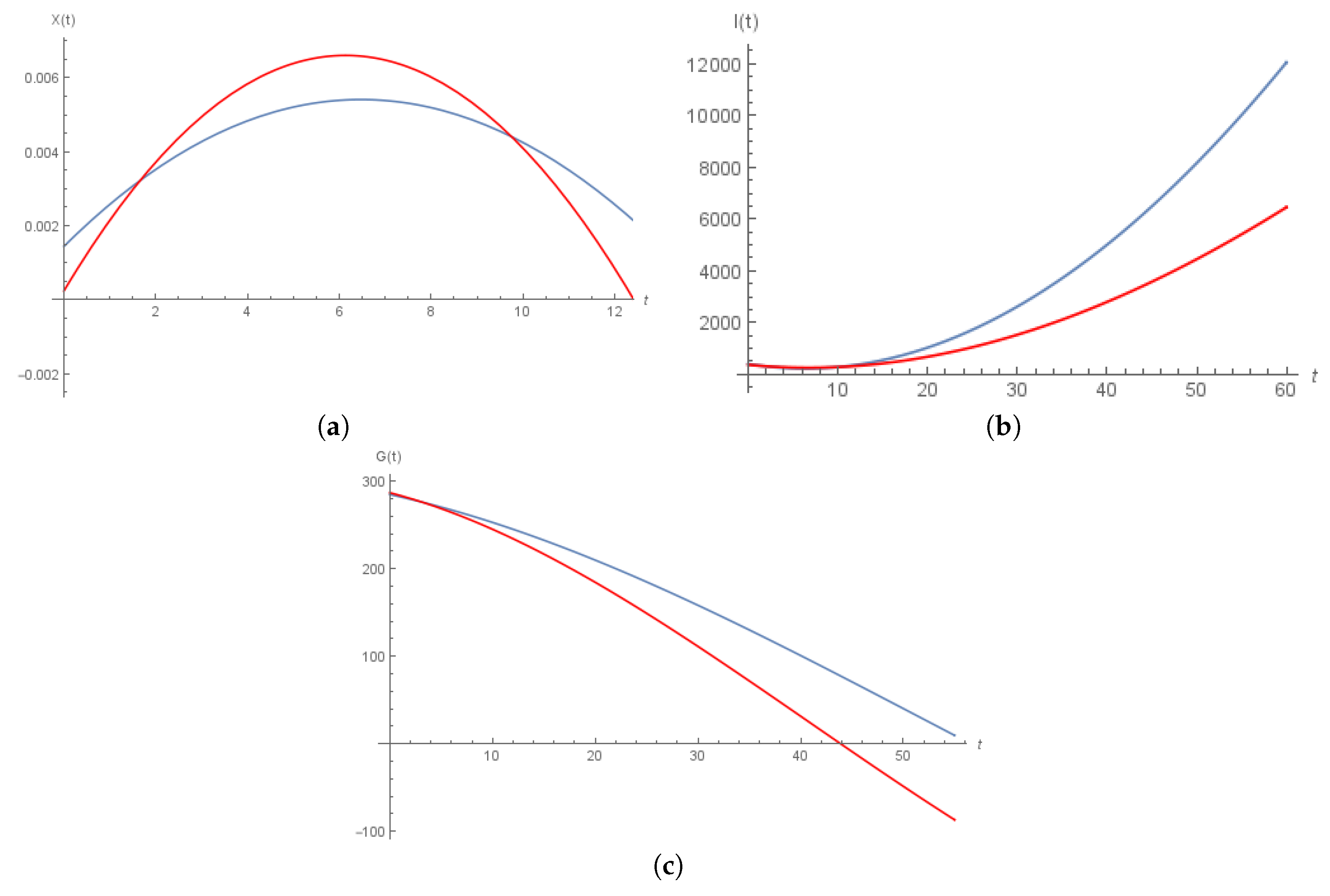
Figure 1. (a) X(t) vs. t (Red line— α = β = γ = 0.5 ; Blue Line— α = β = γ = 0.9 ); (b) I(t) vs. t (Red line— α = β = γ = 0.5 ; Blue Line— α = β = γ = 0.9 ); (c) G(t) vs. t (Red`Line— α = β = γ = 0.5 ; Blue Line— α = β = γ = 0.9 ).
Entropy 19 00114 g001
Table 1. Parameter used in minimal model (11).
ParameterUnitDescription
G(t)(mg/dL)Blood glucose concentration
X(t)(1/min)The effect of active insulin
I(t)(mU/L)Blood insulin concentration
G b (mg/dL)Basal blood glucose concentration
I b (mU/L)Basal blood insulin concentration
p 1 (1/min)Insulin-independent glucose clearance rate
p 2 (1/min)Active insulin clearance rate (upt. decrease)
p 3 (L/(min2·mU))Increase in uptake ability caused by insulin
p 4 (1/min)Decay rate of blood insulin
p 5 (mg/dL)The target glucose level
p 6 (mUdL/L·mg·min)Pancreatic release rate after glucose bolus