
Multicomponent and Longitudinal Imaging Seen as a Communication Channel—An Application to Stroke


1
Univ.Lyon, INSA-Lyon, Université Claude Bernard Lyon 1, CNRS, Inserm, CREATIS UMR 5220, U1206, F-69621 Lyon, France
2
ENS-Lyon, UMR CNRS 5669 ‘UMPA’, and INRIA Alpes, project NUMED, F-69364 Lyon, France
*
Author to whom correspondence should be addressed.
Entropy 2017, 19(5), 187; https://doi.org/10.3390/e19050187
Submission received: 10 March 2017
/
Revised: 18 April 2017
/
Accepted: 24 April 2017
/
Published: 26 April 2017
(This article belongs to the Section Information Theory, Probability and Statistics)
Abstract
:In longitudinal medical studies, multicomponent images of the tissues, acquired at a given stage of a disease, are used to provide information on the fate of the tissues. We propose a quantification of the predictive value of multicomponent images using information theory. To this end, we revisit the predictive information introduced for monodimensional time series and extend it to multicomponent images. The interest of this theoretical approach is illustrated on multicomponent magnetic resonance images acquired on stroke patients at acute and late stages, for which we propose an original and realistic model of noise together with a spatial encoding for the images. We address therefrom very practical questions such as the impact of noise on the predictability, the optimal choice of an observation scale and the predictability gain brought by the addition of imaging components.
1. Introduction
In the medical context, one often needs to predict the future health of tissues based on information contained in one or more imaging components from one or more acquisition time points. An important problem in this type of multicomponent and longitudinal imaging studies is not only to process jointly several components, but also to a priori quantify the benefits (if any) of multi-component and multi-time point integration. This problem is particularly challenging when faced, as is always the case in medical imaging studies, with biological variability and noise in the imaging system.
In such a context, the informational content of physical signals can be defined and quantified in a powerful way by means of statistical information theory, as pioneered by Shannon [1,2]. Statistical information theory proposes measures of similarity and predictability, which are common tools in image processing [3,4]. However, images are not immediately given as statistical objects, and, therefore, each novel situation calls for its specific statistical modeling. This requires the description of a communication channel with at least an input and an output characterized by their statistics expressed on a definite (discrete or continuous) alphabet of symbols together with a noise model. The modeling of imaging problems in the framework of information theory is an active research topic and was recently applied for instance to spectral reduction [5,6], observation scale optimization [7], image visualization [8,9] and multimodality imaging [10,11].
In this work, we propose to study the problem of tissue health prediction in the framework of a Shannon-like communication channel. First, we formalize multicomponent and longitudinal imaging studies in this general framework and revisit the notion of predictive information introduced by Bialek [12]. Then, we illustrate the use of this framework in acute stroke studies. We propose to study the problem of the classification of brain tissues depending on their chances of survival after stroke from magnetic resonance (MR) multicomponent images. We demonstrate the interest of such a modeling approach to address generic practical questions such as (i) the quantification of the gain in predictability obtained by the addition of new image components in prediction studies; (ii) the selection of a relevant spatial observation scale to optimally predict tissue fate; and (iii) the quantification of the impact of imaging noise on the predictability.
2. Methods
2.1. Modeling a Shannon-Like Communication Channel for Multicomponent and Longitudinal Biomedical Imaging Studies
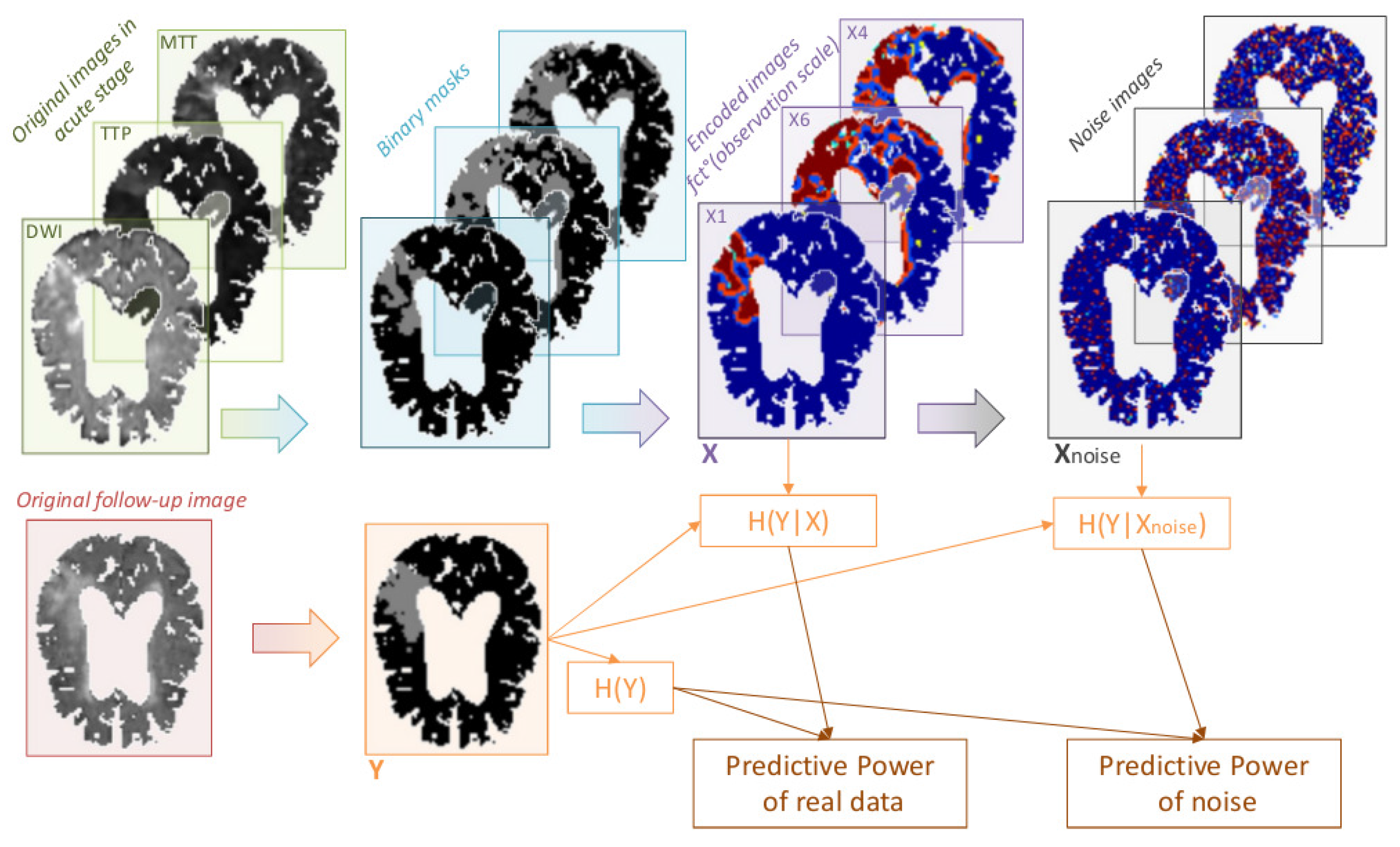
We propose to model multicomponent and longitudinal biomedical imaging studies as a Shannon-like communication channel (see Figure 1), where the input X and the output Y of the communication channel are composed of a multicomponent stack of 3D images acquired, respectively, at an early and a late stage of the evolution of a disease. The underlying hypothesis of the channel proposed in Figure 1 is that the biological process from X to Y is deterministic, assuming therefore that, when the input X is appropriately chosen, only noise in the measuring process of X and Y impairs the predictability of Y given X. Within this framework, we define the predictive power of the input X on the output Y as
where , the entropy of Y, quantifies the amount of information held in the random variable Y and , the conditional entropy of Y on X, quantifies the amount of information needed to describe the outcome of the random variable Y given that the value of the random variable X is known. The value of the predictive power will vary between 0% when X is not informative of Y and 100% when X is a perfect predictor of Y, i.e., . In the literature, there has been numerous proposals for the use of information theory as a measure of temporal evolution [13]. Some are symmetric measures, such as the predictive information [12], and others enable, at the price of numerous acquisition time-points, to determine causal relationships between variables, such as the transfer entropy [14] or the Granger causality [15]. We chose to use a symmetric measure because, in most longitudinal studies, the number of time points is generally limited and the direction of the transfer of information is known. The predictive power proposed here is a normalized version, expressed in percentage rather than in Shannon, of the predictive information introduced by Bialek [12].
In Section 2.2, we explicitly describe the input X and output Y encountered in multicomponent and longitudinal imaging studies for stroke.
2.2. Multicomponent and Longitudinal Imaging Studies in Stroke
Resulting from an abrupt perturbation of blood supply in the brain, stroke is the leading cause of disability in the world. The longer the blood supply stays impaired, the higher the risk of damage to the patient. Treatments can, however, have dangerous side-effects. It is therefore important in clinical routine to rapidly but efficiently evaluate the benefit-risk ratio of administering a treatment to the patient. In this context, diffusion-weighted imaging (DWI) and perfusion-weighted imaging (PWI) are two useful MR imaging modalities used as a diagnostic tool in acute stroke. The biological process leading to infarction is, however, very complex and still misunderstood. Therefore, DWI and PWI MR images are also used in retrospective studies in the aim of gaining a better understanding of stroke mechanisms and improving patient care. These retrospective studies generally investigate the predictive power of DWI and PWI MR images on tissue fate. To do so, they often work from segmented binary masks of the affected areas which can be identified from DWI and PWI images (see Figure 2), as well as a segmented binary mask of the final infarct identified from a follow-up fluid-attenuated inversion recovery (FLAIR) MR image. DWI MR imaging produces one 3D image component on which it is possible to identify areas suffering from a cytotoxic edema. Contrarily, PWI MR imaging produces a 4D image (3D + time) from which we extract, after post-processing, multiple 3D-image components called hemodynamic parameter maps. On each of these maps, it is possible to identify areas suffering from abnormal hemodynamic properties. In practice, five imaging components are commonly generated: the 3D maps of the cerebral blood flow, the cerebral blood volume, the mean transit time, the time to maximum and the time to peak.
The multicomponent and longitudinal stroke studies therefore fit well with the communication channel modeled in Figure 1. The input X of the communication channel can be considered as a six-component stack of binary 3D images segmented at the acute stage of the stroke disease , where is segmented from the DWI MR image and , , , and are segmented from the cerebral blood flow, cerebral blood volume, mean transit time, time to maximum and time to peak maps, respectively, whereas the output Y can be considered as a binary 3D image of the final infarct (one-component stack). Since the image acquisition is realized in emergency conditions, their spatial resolution is low to reduce acquisition time. Furthermore, due to pain or shock, the patients often move during MRI acquisition causing artifacts in the images. The artifacts and poor spatial resolution in stroke studies therefore render the segmentation of the affected areas difficult. In addition, some of the affected areas are less contrasted and more fragmented than others, adding to the difficulty of segmentation [16,17]. Therefore, in stroke studies, the noise level in the input X and output Y is relatively high and a question still under debate is whether the predictive value of X on Y is limited by the fact that there is a high noise level in the images or because X does not capture all the parameters relevant to the biological process of infarction. Furthermore, although largely disseminated in clinic and clinical research for acute stroke, the quantitative benefit of using PWI MRI in addition to DWI MRI is still subject to discussion [18,19]. Since time is of the essence in stroke patient management, an other question of interest is thus to quantify the gain in predictability when integrating PWI imaging components to prediction models. Finally, several stroke prediction studies have shown the interest of taking into account the local spacial environment around voxels rather than considering voxels as independent entities, detached from their surroundings [20,21,22,23]. For this reason, it seems important—particularly when considering the fact that binary masks are a crude summary for gray-scale images, likely to contain segmentation errors near their borders—to quantify the predictability gain in encoding information on the local environment of each voxel.
The communication channel model proposed here offers us a rigorous framework to investigate these clinical questions. Section 2.2.1, Section 2.2.2 and Section 2.2.3 detail the methodology used to address (1) the gain in integrating multiple components in tissue fate prediction studies; (2) the benefit from taking into account the local environment of the tissue and the optimum observation scale; and (3) the impact of imaging noise on the accuracy of tissue fate prediction.
2.2.1. Gain of Predictability with Multicomponent Integration
In order to quantify the gain in predictability when integrating PWI imaging components to prediction models, we propose using the predictive power defined in Equation (1) to select the best combination of n components in terms of tissue fate prediction and evaluating the relative gain in predictability from an n- to an ()-component combination. For the component combination selection, we propose to use a forward-selection approach. Starting from an empty combination set, the forward-selection approach consists of constructing the best component combination by adding at each iteration the component giving the highest predictive power when considering iteratively one, two, three, four, five, then finally six components. In real applications, the data support is finite and the predictive power of noise is consequently non-zero. To evaluate the order of magnitude of the predictive power of noise, we simulate a “noise component” for each component input , composed of voxels with the same distribution as the real component but with a different and random position in space. The mean predictive power of the noise components on the real output Y is then evaluated over 100 noise realizations.
2.2.2. Optimal Observation Scale for Tissue Fate Prediction
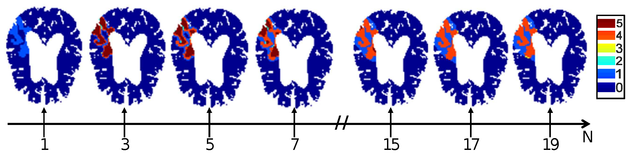
We propose a simple modification of the input components in order to include information on the state of the neighboring voxels, while still preserving a small number of labels (small alphabet). We propose to encode a value for each voxel that depends not only on the value of the voxel itself but also on the value of its neighborhood (neighboring voxels falling outside the brain region being ignored), with N the observation scale. Instead of a two-label encoding (with a label equal to 0 if the voxel is not in the affected area, and to 1 if the voxel is in the affected area), we now propose the six-label encoding described in Table 1.
2.2.3. Impact of Noise on Tissue Fate Prediction Accuracy
We want to quantify to what extent noise impacts the estimated value of the predictive power of the input X on the output Y. However, the difficulty is that, in practice, we do not have access to the real noise-free input and output , but we only observe a noisy version of and , and , with and the error terms on X and Y. To quantify the impact of noise, we need to be able to isolate the drop in predictive power that can be traced back to noise only. To do so, we propose in this work to place ourselves in the simple case where the input X is mono-component and where, without noise, X would be a perfect predictor for the output Y, that is, where %. We simulate inputs X and outputs Y, starting with , and then progressively and independently adding a realistic noise and to both X and Y in order to study the evolution of the predictive power of X on Y as the noise level increases.
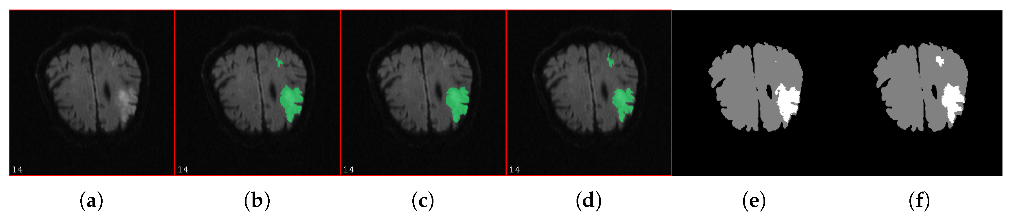
If we ask multiple operators to segment the affected areas on the same image, we observe classically two types of differences between the segmentation masks obtained: (i) local differences situated near the borders of the segmentation masks (see Figure 5b,d) and (ii) global differences with the absence/presence of entire components (see Figure 5b,c). In practice, the status of voxels situated near the border of a segmentation mask is generally less reliable than the status of voxels situated in the core of a segmentation mask.
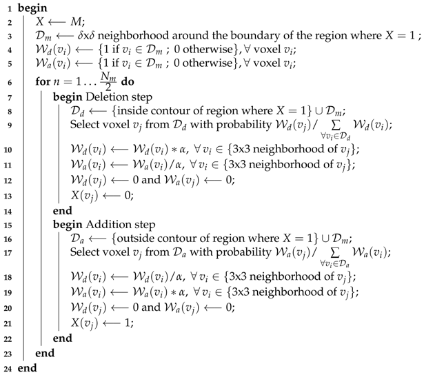
To the best of our knowledge, no simulator of realistic segmentation noise was presented in the literature and we therefore propose a simulator of our own. Realistic global differences with the absence/presence of entire components is harder to simulate than realistic local differences situated near the borders of the segmentation mask. In this work, we introduce only local differences in order to simulate noise. We propose simulating noisy segmentation masks by using randomly positioned modifications (deletions and additions) of voxels from a reference segmentation mask M, where the number of modified voxels () controls the level of noise introduced. We propose two relative measures of the noise level: the proportion of error and the error rate , defined as and , with the number of voxels in the inside contour of the reference segmentation mask and the total number of voxels in the reference segmentation mask. Our simulator produces masks with the same volume as the reference segmentation mask by introducing as many additions as deletions. The positions of the deletions and additions are restricted to the × neighborhood of the border of the reference segmentation mask M in order to simulate realistic local under- and over- estimations of the real affected area. The parameter controls the extent of the area near the mask border that can be subjected to modifications. For our application and given the resolution of the images used in this study, a value of was chosen after inspection of several segmentation masks from different operators. Moreover, for the noisy segmentation masks to be realistic, configurations where deletions and additions occur in a limited number of clustered regions will be favored. In order to do so, each time a voxel is added to (or deleted from) the initial mask M, the probability of its neighboring voxels to be added (or deleted) will be multiplied by a factor of and their probability to be deleted (or added) will be divided by a factor of , with . For deletions and additions will not occur in a limited number of clustered regions and will be evenly distributed around the initial mask border. The higher the value of , the more localized the modifications will be. A value of was chosen after visual inspection to obtain, as can be seen in Figure 5, a satisfying match between real segmentation errors and simulated ones. The detailed procedure for the introduction of noise in a reference mask M is given in Algorithm 1.
| Algorithm 1: Pseudo-algorithm for the introduction of noise in a reference mask M. The inside contour is composed of all the voxels which belong to the segmented region and are in contact with its boundary. The outside contour is composed of all the voxels which do not belong to the segmented region but are in contact with its boundary. The optimum values for and , the two parameters of the algorithm, are application-dependent. Here, they were set to and . In any case, we should have and odd . |
 |
3. Material
3.1. Clinical Data for Tissue Fate Prediction
For the study of the gain of predictability with multicomponents integration and of the optimum observation scale for tissue fate prediction, we use clinical data from the European I-KNOW database [24]. All patients in the multi-center I-KNOW database gave their informed consent and the imaging protocol was approved by the regional ethics commitee. All patients underwent DWI and PWI imaging at admission for acute anterior circulation stroke and follow-up FLAIR imaging one-month after stroke onset. For this pilot study, we selected a limited number of 9 patients who were admitted at the hospital within 3 h of symptom onset. The PWI images were corrected for motion and deconvolved with the circular singular value decomposition-based algorithm to obtain the hemodynamic parameters maps. The hemodynamic maps were then normalized with a hand-drawn reference region. Finally, DWI, PWI and FLAIR images were coregistered for each patient using rigid registration. The binary masks of the final lesion (Y) and of the cytotoxic edema () were segmented manually by experts from the FLAIR and DWI images, respectively. To produce the binary masks from the PWI MR images (, , , and ), each hemodynamic parameter map was thresholded with a threshold value chosen to obtain the best trade-off between sensitivity and specificity for tissue fate prediction. For each map, the threshold was chosen as the value associated with the point closest to the upper-left corner of the sensitivity versus (1-specificity) plot (also called the receiver operating characteristic (ROC)-curve). The ROC-curves were calculated in a region of interest only, with a ratio of infarcting and non-infarcting voxels in accordance with the recommendations of Jonsdottir et al. in their paper on optimal sampling strategy for training data [25]. In the end, in order to study the gain of predictability with multicomponents integration and the optimum observation scale for tissue fate prediction, we used a dataset of approximately 350,000 voxels extracted from the 9 patients processed here.
3.2. Impact of Noise on Tissue Fate Prediction Accuracy
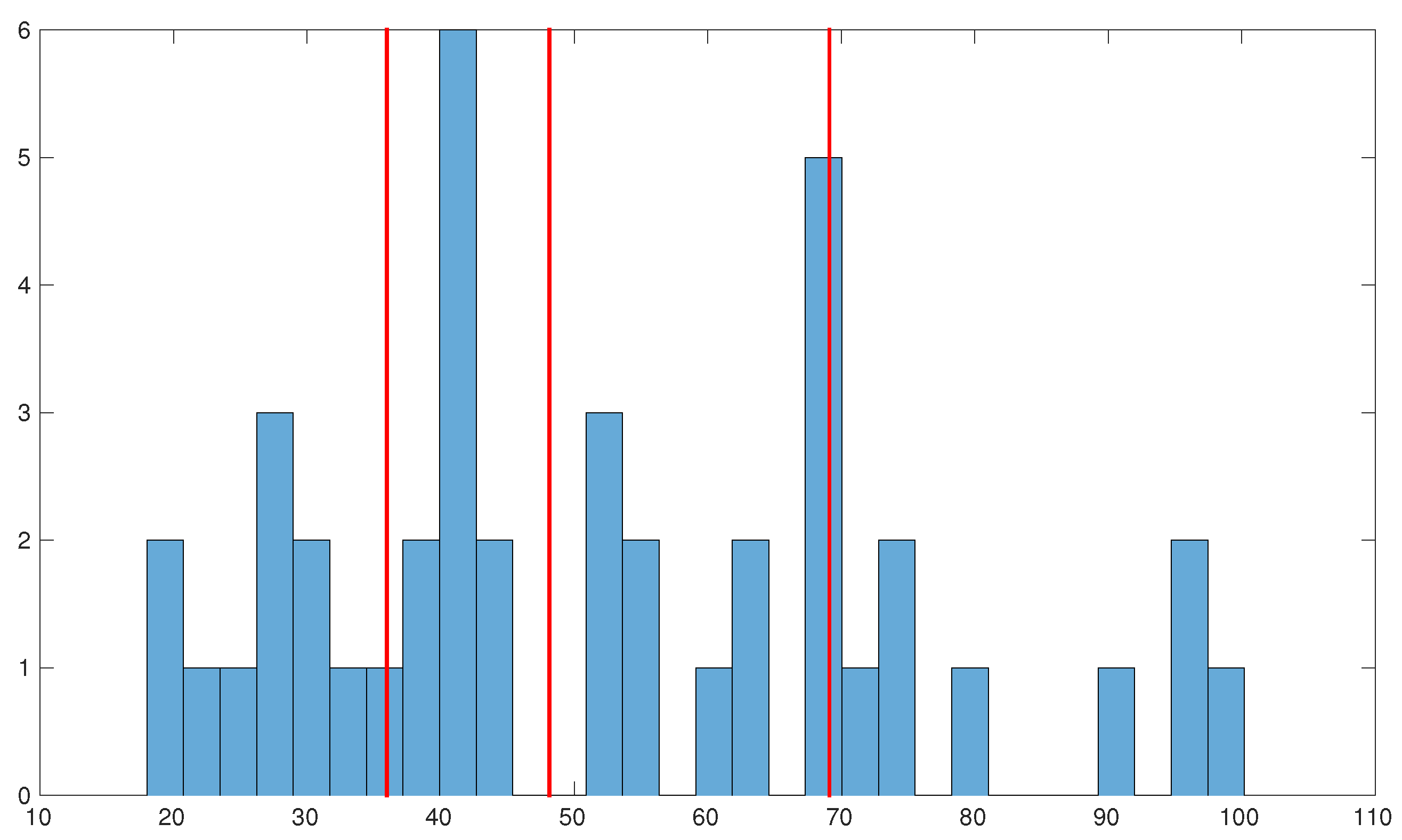
In order to evaluate the impact of noise on tissue fate prediction accuracy, we propose in Section 2.2.3 to study the evolution of the predictive power of a perfect predictor X on an output Y as the level of noise on X and Y increases. Intuitively, we expect that a modification of voxels on a small and fragmented area will have a considerably higher impact on prediction accuracy than a modification of voxels on a large and compact area. Therefore, it is necessary to take into account the variability in size and shape of affected areas in stroke if we want to have a representative estimate of the impact of noise in tissue fate prediction studies. In order to quantify the degree to which a segmented area might be affected by noise, simply as a result of its size and shape, we define the susceptibility factor as , where is the number of voxels in the inside contour of the affected region and the total number of voxels in the affected region. The final lesion masks segmented from a cohort of 42 patients of the I-KNOW database exhibit a great variability of susceptibility factors (cf. Figure 6). We want to evaluate the range of predictive drop due to noise that can be expected in a patient cohort, while still maintaining a reasonable computational cost. To do so, we propose to study the evolution of the predictive power as a function of the level of noise from only three judiciously chosen reference masks among the cohort: those with susceptibility factors closest to the first, the second and the third quartiles, respectively (, and ). We study, for each reference mask , and , the evolution of the predictive power while varying the proportion of error introduced from 0% to 100% with a 5% step. For each value of the proportion error, 30 noise realizations were simulated in order to estimate the mean behavior of the predictive power.
4. Results
4.1. Gain of Predictability with Multicomponent Integration
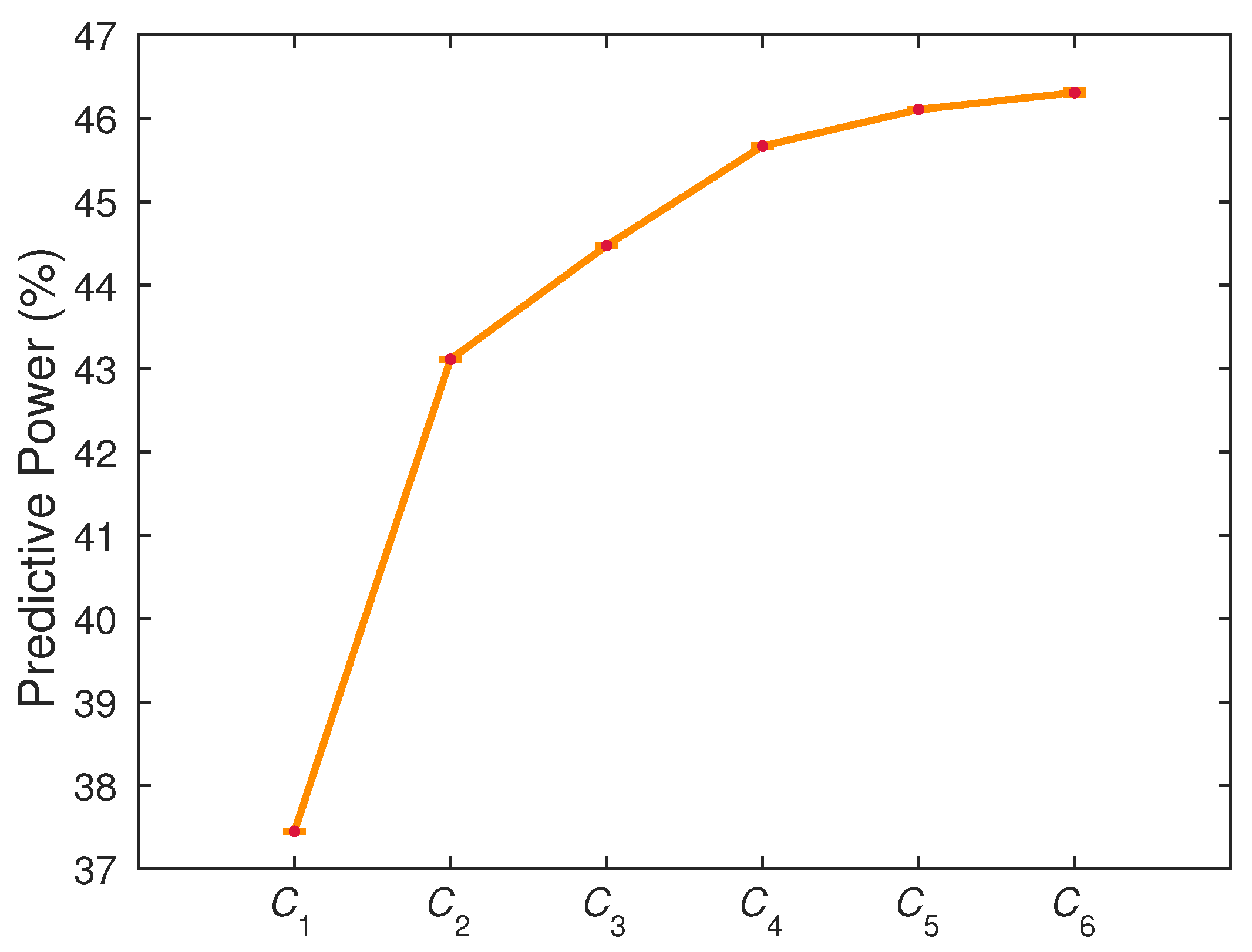
Using a forward-selection approach, we obtain the following optimum combinations: , , , , and , where is the mask extracted from the DWI image, from cerebral blood flow map, from the cerebral blood volume map, from the mean transit time map, from the time to maximum map and from the time to peak map. The predictive power of increases as the number of components n increases (cf. Figure 7). However, the predictive power seems to saturate and reach a plateau around 46% after the integration of five components.
In the literature, the regions in the cytotoxic edema (visible on DWI images) are known to be highly likely to die, even if an efficient treatment is given to the patient, whereas regions suffering from abnormal hemodynamic properties (visible on PWI images) are in danger of infarction but might be salvaged if reperfusion of the tissue occurs. This is in accordance with the results from our forward-selection approach, ranking the DWI segmentation mask as the highest predictive component. In addition, the temporal signal of a PWI 4D image is often modeled in the literature by a gamma-function governed by four parameters [26]. This is in accordance with the results from our forward-selection approach, where the gain in predictability saturates after four components from the PWI have been integrated (), corresponding to the intrinsic dimension of the PWI modality.
4.2. Optimal Observation Scale for Tissue Fate Prediction
Table 2 shows the evolution of the predictive power of combinations to as a function of the observation scale N of the environment of each voxel. No matter the number of components used in the input X, the predictive power starts saturating around N = 13. The saturation level reached depends, however, on the number of components in X and the higher the number of components, the higher the predictive power at saturation. The nine patients included in this study had large and compact final lesions. On average, their lesions measured around 529 voxels per affected slices, that is, if the lesions were a square, they would be a square. The observation scale after which saturation occurs is therefore almost two times smaller than the average lesion size, which seems reasonable. In addition, this observation scale is in accordance with the results reported in [21] where the authors showed that cuboid-based models give better accuracy than voxel-based models and found an optimum cuboid size of for time-to-maximum maps and of for apparent diffusion coefficient MR images. Another important observation is that the mean value of the predictive power of noise increases significantly as we change the size of the coding alphabet (from 2 when N = 1 to 6 when ) and as we increase the number of components considered in the input X. This increase is non-negligible and should be taken into consideration in prediction studies when we work with a limited amount of data.
4.3. Impact of Noise on Tissue Fate Prediction Accuracy
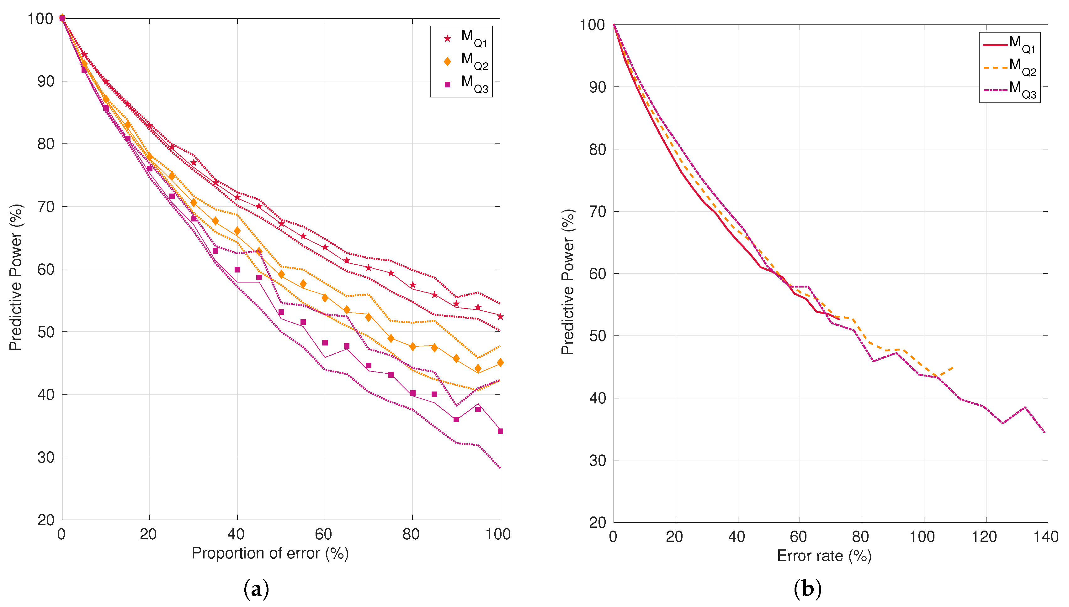
The evolution of the predictive power as a function of the level of noise simulated is displayed in Figure 8. We can see that the predictive power decreases nonlinearly as the level of noise increases. When considering the proportion of error to evaluate the level of noise, one can see that the decrease rate is more important for lesions with a high susceptibility factor () than lesions with a small susceptibility factor (). In addition, the variability due to noise increases as the level of noise increases and it increases faster for lesions with a large susceptibility factor. This suggests that it could be interesting to investigate prediction models with proportional error models rather than additive error models. In Table 2, we found a predictive power of 37.5% for . Such a low predictive power value is never obtained in our simulations from and and is obtained only for very large noise levels in our simulations from . The final lesions of , and were re-segmented manually by two independent operators in an attempt to estimate the order of magnitude of noise in real data. We alternatively took one of the three masks as the reference masks and measured the mean and obtained for , and , respectively. We obtained a mean of 100.9%, 121.1% and 106.2% and a mean ER of 26.9%, 47.4% and 57.3%. Consequently, for a realistic noise level, we obtain with real DWI data a much smaller predictive power than a noisy perfect predictor would give. This suggests that there are other biological processes involved in the infarction mechanism, processes which are not captured by the DWI imaging modality. Here again, this is in accordance with the literature; notably, many studies recently showed the importance of collateral circulation in stroke [27].
5. Discussion
In this article, we have demonstrated the possibility of modeling multicomponent and longitudinal imaging studies using statistical information theory. We modeled multicomponent and longitudinal imaging studies as a communication channel, specifying a model for the perturbations affecting the channel. After this formalization step, we made full use of the framework offered by information theory and demonstrated the efficiency of this modeling approach to answer practical questions encountered in real biomedical problems such as the gain of predictability brought by the addition of new imaging components, the best spatial observation scale for tissue fate prediction or the quantitative impact of noise on the predictability estimated in tissue fate prediction studies. This was illustrated on MRI imaging for stroke disease on a small number of patients. However, all of the results obtained with the statistical information framework were in accordance with results found in the literature and obtained with other image processing tools than information theory. Entropy-based predictability measure the potential of a given set of data for the prediction of a given output. This is somehow similar to what a signal to noise ratio represents, i.e., a measure of detectability, for a detection task. A perspective of this work would be to compare the predictability power obtained from a given dataset with the prediction performances of various modeling tools (random forest, artificial neural networks, support vector machines,⋯) obtained from the same dataset. For stroke, there is currently no consensus for the best modeling tool. However, challenges comparing different approaches, such as the Ischemic Stroke Lesion Segmentation (ISLES) Challenge [28], could be used for a validation of the entropy-based framework proposed here.
Our approach is similar to the predictive information introduced by Bialek in [12] to estimate the intrinsic dimension of time series. So far, the practical applications of predictive information have been mainly focused on monodimensional time series. Here, we have extended the applicability of this theoretic informational framework to multicomponent images and longitudinal studies. A difficulty when extending information theory tools from a monodimensional to a multidimensional problem lies in the encoding of the data. It can tend to generate huge sizes of alphabets leading to the necessity of large amount of data and overwhelming computing costs. In this work, this difficulty was limited due to the fact that we had the possibility to work, as is done in practical stroke applications, on binary images at the input and output of the channel instead of gray level images. In addition, we defined a simple encoding of the environment information of a voxel, adapted to the problematic of tissue fate prediction. This encoding allowed for keeping a constant size of alphabet while scanning the whole range of spatial scale available in the images.
This opens the way for investigations in various directions. Here, we tested a very crude encoding of the voxel environment, and it would be interesting to study the gain in predictability with other local descriptors such as the local binary patterns [29,30], which have the advantage of encoding the environment of voxels in gray level imaging while still maintaining a limited size of alphabet. Furthermore, the question of predictability, as stressed by Bialek in [12], is linked to some fundamental questions in machine learning. The evolution of predictability as a function of the number of imaging components or points in a time series gives insights on the intrinsic complexity or dimension of a problem. Nowadays, machine learning methods are very popular in biomedical imaging and have recently been tested successfully on the biomedical issues illustrated in this work [22,31]. A fundamental question is the size of the training set necessary to allow the learning of the prediction of tissue fate without over-fitting. The communication channel model proposed here constitutes a possible tool in this context to estimate the intrinsic dimension or complexity of a problem that could serve in many biomedical applications.
Acknowledgments
This work was supported by the LABEX PRIMES (ANR-11-LABX-0063) of the Université de Lyon, within the program “Investissements d’Avenir” (ANR-11-IDEX-0007) operated by the French National Research Agency (ANR).
Author Contributions
Mathilde Giacalone, Carole Frindel, Emmanuel Grenier and David Rousseau conceived and designed the experiments; Mathilde Giacalone performed the experiments; Mathilde Giacalone and David Rousseau analyzed the data; and Mathilde Giacalone, Carole Frindel and David Rousseau wrote the paper. All authors have read and approved the final manuscript.
Conflicts of Interest
The authors declare no conflict of interest.
References
- Shannon, C.E. A Mathematical Theory of Communication. Bell Syst. Tech. J. 1948, 27, 379–423, 623–656. [Google Scholar] [CrossRef]
- Cover, T.M.; Thomas, J.A. Elements of Information Theory; Wiley: Hoboken, NJ, USA, 2012. [Google Scholar]
- Ruiz, F.E.; Pérez, P.S.; Bonev, B.I. Information Theory in Computer Vision and Pattern Recognition; Springer: Berlin/Heidelberg, Germany, 2009. [Google Scholar]
- Mohammad-Djafari, A. Entropy, information theory, information geometry and Bayesian inference in data, signal and image processing and inverse problems. Entropy 2015, 17, 3989–4027. [Google Scholar] [CrossRef]
- Benoit, L.; Belin, É.; Rousseau, D.; Chapeau-Blondeau, F. Information-theoretic modeling of trichromacy coding of light spectrum. Fluct. Noise Lett. 2014, 13, 1450025. [Google Scholar] [CrossRef]
- Benoit, L.; Benoit, R.; Belin, É.; Vadaine, R.; Demilly, D.; Chapeau-Blondeau, F.; Rousseau, D. On the value of the Kullback–Leibler divergence for cost-effective spectral imaging of plants by optimal selection of wavebands. Mach. Vis. Appl. 2016, 27, 625–635. [Google Scholar] [CrossRef]
- Delahaies, A.; Rousseau, D.; Chapeau-Blondeau, F. Joint acquisition-processing approach to optimize observation scales in noisy imaging. Opt. Lett. 2011, 36, 972–974. [Google Scholar] [CrossRef] [PubMed]
- Justesen, J.; Forchhammer, S. Two-Dimensional Information Theory and Coding: With Applications to Graphics Data and High-Density Storage Media; Cambridge University Press: Cambridge, UK, 2010. [Google Scholar]
- Chen, M.; Feixas, M.; Viola, I.; Bardera, A.; Shen, H.W.; Sbert, M. Information Theory Tools for Visualization; CRC Press: Boca Raton, FL, USA, 2016. [Google Scholar]
- Bramon, R.; Boada, I.; Bardera, A.; Rodriguez, J.; Feixas, M.; Puig, J.; Sbert, M. Multimodal data fusion based on mutual information. IEEE Trans. Vis. Comput. Graph. 2012, 18, 1574–1587. [Google Scholar] [CrossRef] [PubMed]
- Chlaily, S.; Amblard, P.O.; Michel, O.; Jutten, C. Impact of noise correlation on multimodality. In Proceedings of the 24th European Signal Processing Conference (EUSIPCO), Budapest, Hungary, 29 August–2 September 2016; pp. 195–199. [Google Scholar]
- Bialek, W.; Nemenman, I.; Tishby, N. Predictability, complexity, and learning. Neural Comput. 2001, 13, 2409–2463. [Google Scholar] [CrossRef] [PubMed]
- Rosas, F.; Ntranos, V.; Ellison, C.J.; Pollin, S.; Verhelst, M. Understanding interdependency through complex information sharing. Entropy 2016, 18, 38. [Google Scholar] [CrossRef]
- Schreiber, T. Measuring information transfer. Phys. Rev. Lett. 2000, 85, 461. [Google Scholar] [CrossRef] [PubMed]
- Amblard, P.O.; Michel, O.J. The relation between Granger causality and directed information theory: A review. Entropy 2012, 15, 113–143. [Google Scholar] [CrossRef]
- Rivers, C.S.; Wardlaw, J.M.; Armitage, P.A.; Bastin, M.E.; Hand, P.J.; Dennis, M.S. Acute ischemic stroke lesion measurement on diffusion-weighted imaging–important considerations in designing acute stroke trials with magnetic resonance imaging. J. Stroke Cereb. Dis. 2007, 16, 64–70. [Google Scholar] [CrossRef] [PubMed]
- Neumann, A.B.; Jonsdottir, K.Y.; Mouridsen, K.; Hjort, N.; Gyldensted, C.; Bizzi, A.; Fiehler, J.; Gasparotti, R.; Gillard, J.H.; Hermier, M.; et al. Interrater agreement for final infarct MRI lesion delineation. Stroke 2009, 40, 3768–3771. [Google Scholar] [CrossRef] [PubMed]
- Willats, L.; Calamante, F. The 39 steps: Evading error and deciphering the secrets for accurate dynamic susceptibility contrast MRI. NMR Biomed. 2013, 26, 913–931. [Google Scholar] [CrossRef] [PubMed]
- Giacalone, M.; Frindel, C.; Zagala, R.; Cho, T.H.; Berthezène, Y.; Nighoghossian, N.; Rousseau, D. On the Influence of Normalization Strategies for Perfusion MRI in Acute Stroke. In Current Developments in Stroke; Bentham Science: Sharjah, United Arab Emirates, 2017. [Google Scholar]
- Scalzo, F.; Hao, Q.; Alger, J.R.; Hu, X.; Liebeskind, D.S. Tissue fate prediction in acute ischemic stroke using cuboid models. In Advances in Visual Computing, ISVC 2010; Lecture Notes in Computer Science; Springer: Berlin/Heidelberg, Germany, 2010; Volume 6454, pp. 292–301. [Google Scholar]
- Scalzo, F.; Hao, Q.; Alger, J.R.; Hu, X.; Liebeskind, D.S. Regional prediction of tissue fate in acute ischemic stroke. Ann. Biomed. Eng. 2012, 40, 2177–2187. [Google Scholar] [CrossRef] [PubMed]
- Huang, S.; Shen, Q.; Duong, T.Q. Artificial neural network prediction of ischemic tissue fate in acute stroke imaging. J. Cereb. Blood Flow Metab. 2010, 30, 1661–1670. [Google Scholar] [CrossRef] [PubMed]
- Nguyen, V.H.; Cooperman, G.; Menenzes, N.; Lopez, C.J.; Melinosky, C.; Wu, O.; Ay, H.; Liu, Y.; Nuutinen, J.; Aronen, H.J.; et al. Stroke tissue outcome prediction using a spatially-correlated model. In Proceedings of the 2008 Pan-Pacific Imaging Conference, Tokyo, Japan, 25–27 June 2008; pp. 238–241. [Google Scholar]
- Frindel, C.; Rouanet, A.; Giacalone, M.; Cho, T.H.; Østergaard, L.; Fiehler, J.; Pedraza, S.; Baron, J.C.; Wiart, M.; Berthezène, Y.; et al. Validity of shape as a predictive biomarker of final infarct volume in acute ischemic stroke. Stroke 2015, 46, 976–981. [Google Scholar] [CrossRef] [PubMed]
- Jonsdottir, K.Y.; Østergaard, L.; Mouridsen, K. Predicting Tissue Outcome From Acute Stroke Magnetic Resonance Imaging. Stroke 2009, 40, 3006–3011. [Google Scholar] [CrossRef] [PubMed]
- Giacalone, M.; Frindel, C.; Robini, M.; Cervenansky, F.; Grenier, E.; Rousseau, D. Robustness of spatio-temporal regularization in perfusion MRI deconvolution: An application to acute ischemic stroke. Magn. Reson. Med. 2016. [Google Scholar] [CrossRef] [PubMed]
- Bang, O.Y.; Goyal, M.; Liebeskind, D.S. Collateral circulation in ischemic stroke. Stroke 2015, 46, 3302–3309. [Google Scholar] [CrossRef] [PubMed]
- Maier, O.; Menze, B.H.; von der Gablentz, J.; Häni, L.; Heinrich, M.P.; Liebrand, M.; Winzeck, S.; Basit, A.; Bentley, P.; Chen, L.; et al. ISLES 2015-A public evaluation benchmark for ischemic stroke lesion segmentation from multispectral MRI. Med. Image Anal. 2017, 35, 250–269. [Google Scholar] [CrossRef] [PubMed]
- Ojala, T.; Pietikäinen, M.; Harwood, D. A comparative study of texture measures with classification based on featured distributions. Pattern Recogn. 1996, 29, 51–59. [Google Scholar] [CrossRef]
- Pietikäinen, M.; Zhao, G. Two decades of local binary patterns: A survey. In Advances in Independent Component Analysis and Learning Machines; Elsevier: Amsterdam, The Netherlands, 2015; pp. 175–210. [Google Scholar]
- Bagher-Ebadian, H.; Jafari-Khouzani, K.; Mitsias, P.D.; Lu, M.; Soltanian-Zadeh, H.; Chopp, M.; Ewing, J.R. Predicting final extent of ischemic infarction using artificial neural network analysis of multi-parametric MRI in patients with stroke. PLoS ONE 2011, 6, e22626. [Google Scholar] [CrossRef] [PubMed]
Figure 1.
General Shannon-like communication channel for multicomponent and longitudinal biomedical imaging studies. The imaging process is not deterministic, and the input and output are perturbed by noise.
Figure 1.
General Shannon-like communication channel for multicomponent and longitudinal biomedical imaging studies. The imaging process is not deterministic, and the input and output are perturbed by noise.
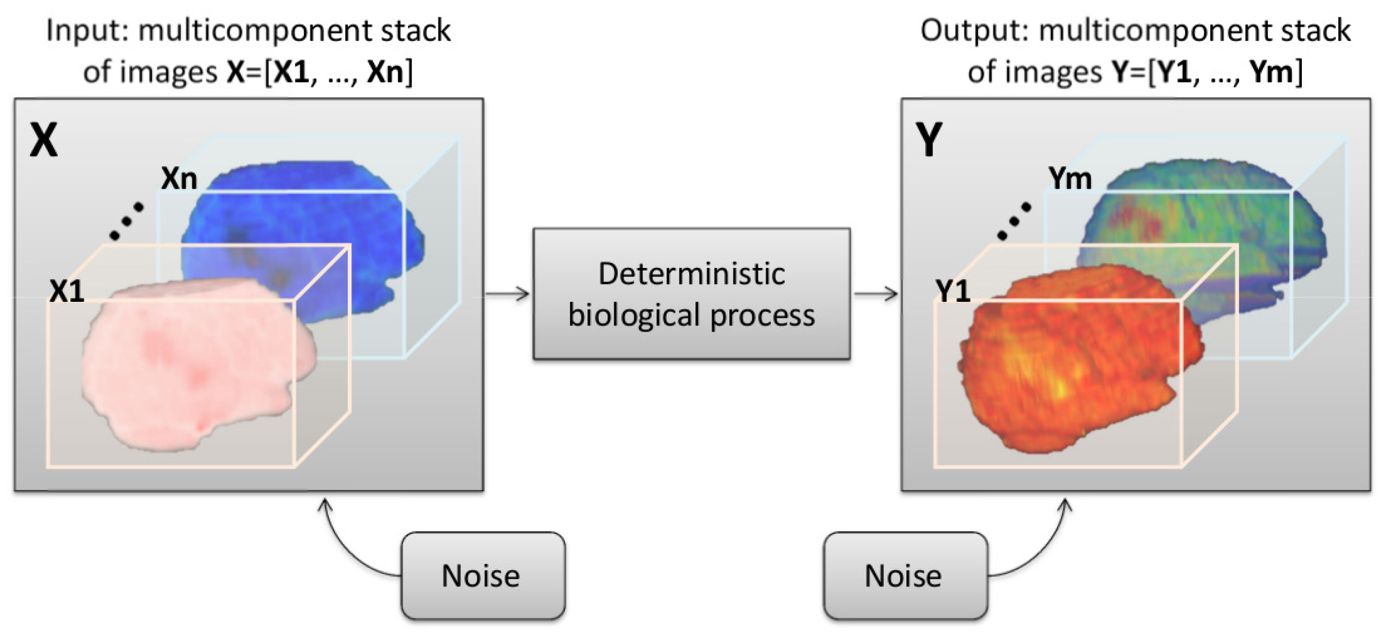
Figure 2.
Illustration of the binary mask of a cytotoxic edema (c) segmented from the diffusion-weighted imaging of a patient in acute stage (a); (b) show the superposition of the affected area on the image used for the segmentation.
Figure 2.
Illustration of the binary mask of a cytotoxic edema (c) segmented from the diffusion-weighted imaging of a patient in acute stage (a); (b) show the superposition of the affected area on the image used for the segmentation.
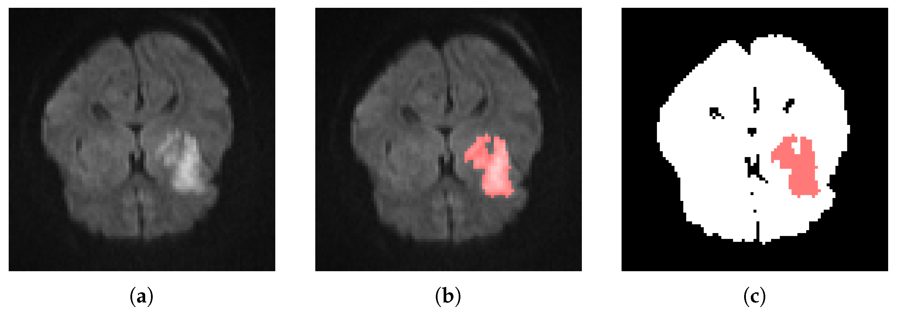
Figure 3.
Illustration of the evolution of the labels in an image component as the observation scale N is increased.
Figure 3.
Illustration of the evolution of the labels in an image component as the observation scale N is increased.

Figure 4.
Illustration of the processing pipeline proposed for the study of the gain in predictability from observation scale optimization in tissue fate prediction studies for stroke. The study of the gain in predictability from component integration presented in Section 2.2.1 corresponds to the specific case where the observation scale equals 1 and the encoded images are thus exactly the same as the binary masks.

Figure 5.
(a–d): illustration of segmentation masks of a same image (a) when segmented by three different experts (b–d). One can see that the small affected area segmented by the experts in masks (b,d), was not segmented by the expert on mask (c). In addition, one can clearly see differences between masks (b–d) around the border of the largest affected area. (e,f): illustration of noisy masks simulated from the segmentation mask (b) with Algorithm 1.

Figure 6.
Histogram of the susceptibility factor of the final lesion masks for a cohort of 42 patients, with the red lines corresponding (from left to right) to the first, second and third quartiles, respectively.
Figure 6.
Histogram of the susceptibility factor of the final lesion masks for a cohort of 42 patients, with the red lines corresponding (from left to right) to the first, second and third quartiles, respectively.

Figure 7.
Evolution of the predictive power as the number of components in the communication channel input is increased.
Figure 7.
Evolution of the predictive power as the number of components in the communication channel input is increased.

Figure 8.
Evolution of the predictive power as a function of the proportion of error (a) or corresponding error rate introduced (b), in red for the mask representative of the first quartile (), in orange for the mask representative of the second quartile () and in purple for the mask representative of the third quartile () of the susceptibility factor distribution. The points correspond to the mean values, the line to the median values and the dotted lines to the first and third quartiles values obtained over 30 noise realizations for each value of the proportion of error tested.


Table 1.
Six-label encoding for binary masks taking into account, for each voxel, the state of the voxels in its neighborhood.
Table 1.
Six-label encoding for binary masks taking into account, for each voxel, the state of the voxels in its neighborhood.
| Label | Voxel in Affected Area | % Of Neighboring Voxels in Affected Area |
|---|---|---|
| 0 | no | |
| 1 | no | |
| 2 | no | |
| 3 | yes | |
| 4 | yes | |
| 5 | yes |
Table 2.
Predictive power obtained for real data ± mean predictive power of noise evaluated over 100 noise realizations. = optimum combination of n predictor variables. N = observation scale for the voxel neighborhood.
Table 2.
Predictive power obtained for real data ± mean predictive power of noise evaluated over 100 noise realizations. = optimum combination of n predictor variables. N = observation scale for the voxel neighborhood.
| N | ||||||
|---|---|---|---|---|---|---|
| 1 | 37.4508 ± 0.0004 | 43.1119 ± 0.0009 | 44.475 ± 0.002 | 45.669 ± 0.005 | 46.108 ± 0.001 | 46.31 ± 0.02 |
| 3 | 42.294 ± 0.002 | 48.46 ± 0.01 | 49.90 ± 0.06 | 51.5 ± 0.2 | 52.7 ± 0.8 | 54 ± 2 |
| 5 | 44.903 ± 0.002 | 51.40 ± 0.01 | 52.93 ± 0.06 | 54.6 ± 0.3 | 56 ± 1 | 58 ± 3 |
| 7 | 46.846 ± 0.002 | 53.48 ± 0.01 | 55.10 ± 0.06 | 56.9 ± 0.3 | 58 ± 1 | 60 ± 3 |
| 9 | 48.206 ± 0.002 | 54.95 ± 0.01 | 56.60 ± 0.07 | 58.5 ± 0.3 | 60 ± 1 | 62 ± 4 |
| 11 | 49.103 ± 0.002 | 55.94 ± 0.01 | 57.59 ± 0.07 | 59.6 ± 0.3 | 61 ± 1 | 63 ± 4 |
| 13 | 49.668 ± 0.002 | 56.57 ± 0.01 | 58.33 ± 0.07 | 60.4 ± 0.3 | 62 ± 1 | 64 ± 4 |
| 15 | 50.101 ± 0.002 | 56.92 ± 0.01 | 58.78 ± 0.07 | 60.9 ± 0.3 | 63 ± 1 | 65 ± 4 |
| 17 | 50.437 ± 0.002 | 57.29 ± 0.01 | 59.23 ± 0.07 | 61.4 ± 0.3 | 63 ± 1 | 65 ± 4 |
| 19 | 50.558 ± 0.002 | 57.55 ± 0.01 | 59.50 ± 0.07 | 61.8 ± 0.3 | 64 ± 1 | 65 ± 4 |
© 2017 by the authors. Licensee MDPI, Basel, Switzerland. This article is an open access article distributed under the terms and conditions of the Creative Commons Attribution (CC BY) license (http://creativecommons.org/licenses/by/4.0/).
Share and Cite
MDPI and ACS Style
Giacalone, M.; Frindel, C.; Grenier, E.; Rousseau, D. Multicomponent and Longitudinal Imaging Seen as a Communication Channel—An Application to Stroke. Entropy 2017, 19, 187. https://doi.org/10.3390/e19050187
AMA Style
Giacalone M, Frindel C, Grenier E, Rousseau D. Multicomponent and Longitudinal Imaging Seen as a Communication Channel—An Application to Stroke. Entropy. 2017; 19(5):187. https://doi.org/10.3390/e19050187
Chicago/Turabian StyleGiacalone, Mathilde, Carole Frindel, Emmanuel Grenier, and David Rousseau. 2017. "Multicomponent and Longitudinal Imaging Seen as a Communication Channel—An Application to Stroke" Entropy 19, no. 5: 187. https://doi.org/10.3390/e19050187
Note that from the first issue of 2016, this journal uses article numbers instead of page numbers. See further details here.