Image Bi-Level Thresholding Based on Gray Level-Local Variance Histogram

Abstract

Thresholding is a popular method of image segmentation. Many thresholding methods utilize only the gray level information of pixels in the image, which may lead to poor segmentation performance because the spatial correlation information between pixels is ignored. To improve the performance of thresolding methods, a novel two-dimensional histogram—called gray level-local variance (GLLV) histogram—is proposed in this paper as an entropic thresholding method to segment images with bimodal histograms. The GLLV histogram is constructed by using the gray level information of pixels and its local variance in a neighborhood. Local variance measures the dispersion of gray level distribution of pixels in a neighborhood. If a pixel’s gray level is close to its neighboring pixels, its local variance is small, and vice versa. Therefore, local variance can reflect the spatial information between pixels. The GLLV histogram takes not only the gray level, but also the spatial information into consideration. Experimental results show that an entropic thresholding method based on the GLLV histogram can achieve better segmentation performance.

1. Introduction

Image segmentation is the process of grouping an image’s pixels into homogenous regions with respect to one or more characteristics, such as texture, color, and brightness. It plays a critical role in image, video, and computer vision applications such as defect detection [1,2], character recognition [3], document analysis [4], etc. Many methods have been developed for image segmentation. Among these methods, the thresholding method is widely used for its simplicity and ease of implementation. The basic assumption of thresholding method is that the object and background can be classified by their intensity values. Thresholding methods can be classified into two classes: bi-level thresholding and multi-level thresholding. For bi-level thresholding, only one threshold is selected to segment the image into two classes, while for multi-level thresholding, more than one threshold should be determined to segment the image into multiple classes because the histogram of the image has more than two modes [5].

To select a suitable threshold, thresholding methods usually optimize a criterion function; for example, maximizing between-class variance [6], or minimum classification error [7]. Entropy is a measure of uncertainty in an information source, and has received increasing attention from researchers for the selection of thresholding values. Pun [8,9] first proposed the selection of thresholds using an entropy criterion. In his proposed method, the upper bound of the posteriori entropy of the object and background were maximized. Wong and Sahoo [10] refined Pun’s method and determined the optimal threshold by maximizing the posteriori entropy under inequality constraints, which characterize the uniformity and shape of the segmented regions. Kapur et al. [11] put forward a new method called maximum entropy thresholding, which selects the optimum threshold by maximizing the sum of entropies of the object and the background. Li and Lee [12] proposed the cross-entropy thresholding method by minimizing the information difference between the input image and the output binary image.

Entropic thresholding methods are effective for most real-world images, but a few shortcomings remain. Most importantly, entropic thresholding methods only utilize the distribution of gray level (i.e., one-dimensional (1D) histogram) of an image. As a result, different images with the same histogram may have the same threshold, which is not reasonable. To overcome this shortcoming, many researchers devoted their efforts to integrating spatial correlation information between pixels into the thresholding process. The pioneer work on this point belongs to Abutaleb [13]. Abutaleb proposed the concept of a two-dimensional (2D) histogram, which incorporates spatial information as well as the gray-level of pixels to enhance the performance of Kapur’s entropic thresholding method. Then, the 2D histogram was adopted by several authors to improve the performance of thresholding methods based on 1D histograms. In [14], a two-dimensional Reny’s entropy thresholding method was proposed. A two-dimensional Otsu’s thresholding method was proposed in [15]. In [16], Tang et al. extended the minimum Tsallis cross-entropy thresholding method to a two-dimensional case. Sahoo and Arora [17] proposed a 2D Tsallis entropy thresholding method.

Though improved performance can be obtained, all 2D thresholding methods still have a distinct disadvantage; i.e., they only utilize the information related to background and object, and ignore the information related to edges, in which important information may be contained. Hence, several authors proposed the use of other information reflecting spatial correlation between pixels to construct a 2D histogram. Xiao et al. [18] proposed the gray level spatial correlation (GLSC) histogram, which was constructed using the gray value of pixels and and their similarity with neighboring pixels. In Reference [19], a 2D direction (2D-D) histogram was proposed by using the local edge property computed from the orientation histogram of a gradient image. After analyzing the drawbacks of GLSC and 2D-D, Xiao et al. [20] proposed another 2D histogram; i.e., the gray-level and gradient magnitude (GLGM) histogram. GLGM utilizes the gradient magnitudes instead of gradient orientation. It was claimed that the 2D-D histogram and the GLGM histogram are more effective than Abutaleb’s 2D histogram. Nevertheless, the construction of 2D-D and GLGM histograms are not as convenient as Abutaleb’s 2D histogram. For the 2D-D histogram, the gradient orientation is divided into K bins, and the magnitude of the gradient should be filtered using a Gaussian filter with parameter $\sigma$. It is difficult to select an appropriate value for K and $\sigma$. In addition, to construct the GLGM histogram, anisotropic diffusion filtering (ADF) is performed as a preprocessing step. In ADF, the selection of a conductivity function and its parameter is also difficult. Furthermore, our research results show that the filtering operation in the construction of the 2D-D and GLGM histograms has a great effect on the performance of entropic thresholding methods.

In this paper, a novel thresholding method is presented by taking the spatial information between pixels into consideration. To this end, a novel 2D histogram—called gray level local variance (GLLV) histogram—is constructed from the gray level of pixels and the local variance of its neighboring pixels. The GLLV histogram can effectively capture edge information, and its computation burden is less than that of 2D-D and GLGM histogram.

The rest of this paper is organized as follows. The construction of the GLLV histogram is presented in Section 2. Image thresholding based on GLLV is given in Section 3. The experimental results are presented in Section 4. Finally, the concluding remarks are given in Section 5.

2. GLLV Histogram

As stated before, taking spatial information into account can enhance the performance of thresholding methods. The spatial information of an image can be represented by its local features, such as local mean [13], gradients [19,20], etc. In this paper, we propose another method to construct a 2D histogram to integrate spatial information into the thresholding process. The proposed method is based on the local variance of a pixel and not the gradient information, as in 2D-D and GLGM histograms.

2.1. Local Feature of Image via Local Variance

In probability theory, variance is a measure of the dispersion of a random variable. If the observations of a random variable are more dispersed, the variance is larger, and vice versa. Generally speaking, in an image, the gray values of pixels inside the objects or background are homogeneous. In other words, their gray values are close to its neighboring pixels, and therefore the local variance of the pixel is small. However, with respect to the pixels located at the boundary between the object and the background, their gray values are obviously different from its neighboring pixels. So, their local variance is large. It is seen that local variance can reflect some certain properties of the edges [21]. Based on this observation, in the following, a new 2D histogram called gray level—local variance (GLLV) histogram is constructed.

2.2. Construction of GLLV Histogram

Let I be an image of size $M\times N$ with gray level ranging in $\{0,1,\cdots ,L-1\}$ and $I(x,y)$ be the gray value of the pixel located at $(x,y)$, where $x=1,2,\dots ,M$ and $y=1,2,\dots ,N$.

For each pixel at $(x,y)$, its local variance with neighborhood size $n\times n$ is calculated as

$$g(x,y)=\frac{1}{n^2-1}\sum _{i=-(n-1)/2}^{(n-1)/2}\sum _{j=-(n-1)/2}^{(n-1)/2}{[I(x+i,y+j)-\overline{I}(x,y)]}^2$$

(1)

where $\overline{I}(x,y)$ is the mean of pixels in the neighborhood, and is calculated as

$$\overline{I}(x,y)=\frac{1}{n^2}\sum _{i=-(n-1)/2}^{(n-1)/2}\sum _{j=-(n-1)/2}^{(n-1)/2}I(x+i,y+j)$$

(2)

The local variance of each pixel is normalized as

$$g(x,y)=\mathrm{INT}[(g(x,y)-g_{min})\times L^{\prime }/(g_{max}-g_{min})]$$

(3)

where $\mathrm{INT}[·]$ is an operator to get the integer part, and $g_{max}$ and $g_{min}$ denote the maximum and minimum of $g(x,y)$, respectively. $L^{\prime }$ is chosen as 64 according to the experimental conclusion. Letting $n_{ij}$ be the total number of pixel pairs that $I(x,y)=i$ and $g(x,y)=j$ in the image, then the GLLV histogram is defined as

$$p_{ij}=\frac{n_{ij}}{M\times N}.$$

(4)

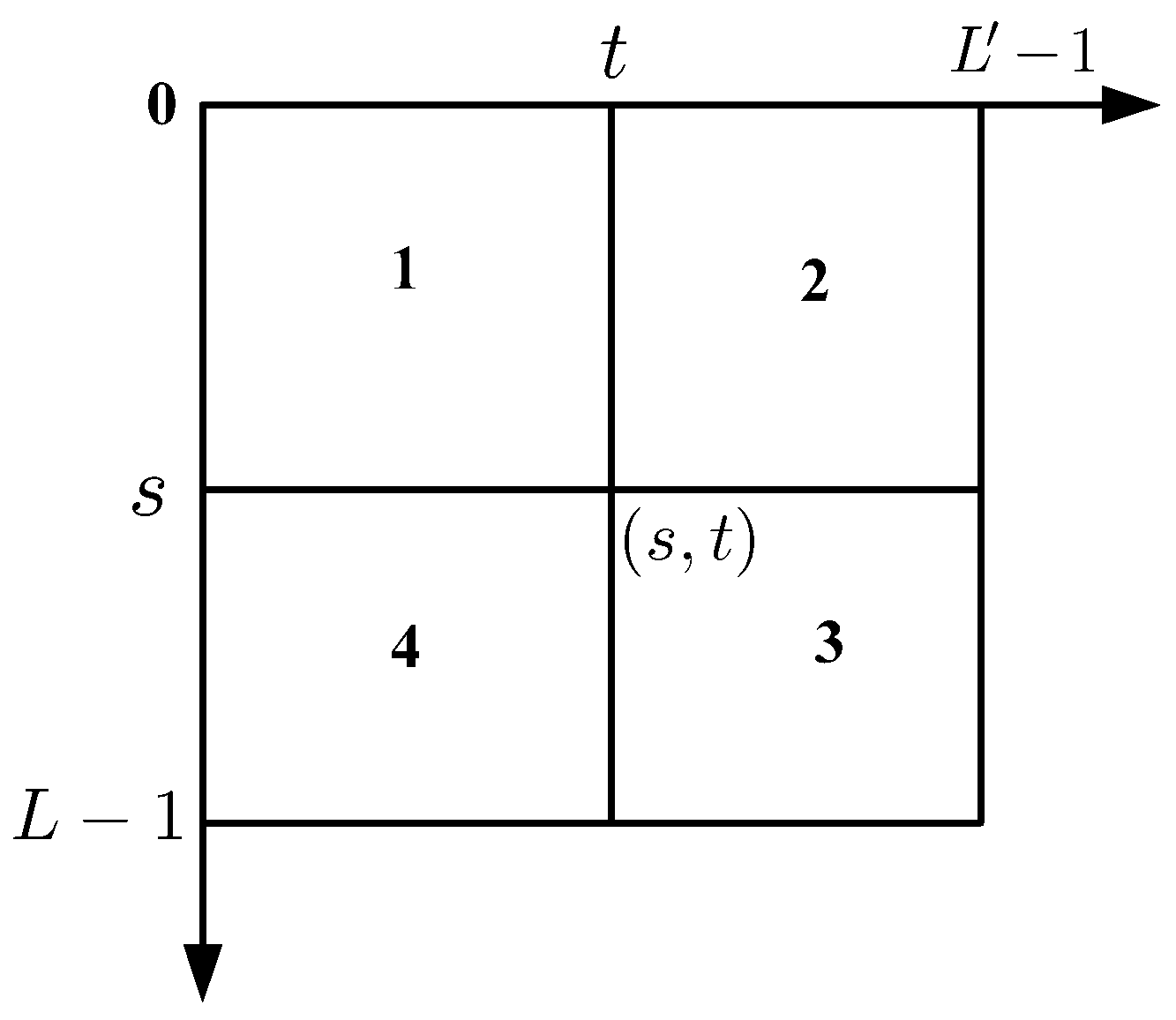
GLLV histogram $P=\{p_{ij};i=0,1,\cdots ,L-1;j=0,1,\cdots ,L^{\prime }-1\}$ is a matrix with size $L\times L^{\prime }$, which is shown in Figure 1.

Suppose a 2D threshold vector $(s,t)$ divides the GLLV histogram into four regions, where s represents the threshold of the original image and t the threshold of the local variance. Observing that pixels inside the objects and background have small local variance, in the GLLV histogram, Regions 1 and 4 therefore contain the information of objects and background, respectively. Regions 2 and 3 contain information of edges and noise. Since our main task is to segment object from background, we therefore pay much attention to Regions 1 and 4 and ignore Regions 2 and 3. Specifically, The histogram bins with j between $t+1$ and $L^{\prime }-1$ cover Regions 2 and 3.

3. Image Thresholding Based on GLLV

Suppose there are two classes in the image; i.e., the background $C_0$ and object $C_1$. As mentioned above, Regions 1 and 4 contain the background and object, respectively. Let $P_0$ and $P_1$ be the probability of the object and background, respectively. They are calculated as

$$P_0(s,t)=\sum _{i=0}^s\sum _{j=0}^t{p}_{ij}$$

(5)

$$P_1(s,t)=\sum _{i=s+1}^{L-1}\sum _{j=0}^t{p}_{ij}=P_T\left(t\right)-P_0(s,t)$$

(6)

where $P_T\left(t\right)={\displaystyle \sum _{i=0}^{L-1}}{\displaystyle \sum _{j=0}^t}{p}_{ij}$. Then, the normalized posteriori class probabilities of the object and background are

$$C_0:\left\{\frac{p_{ij}}{P_0};i=0,1,2,\cdots ,s;j=0,1,2,\cdots ,t\right\},$$

(7)

and

$$C_1:\left\{\frac{p_{ij}}{P_1};i=s+1,\cdots ,L-1;j=0,1,2,\cdots ,t\right\}.$$

(8)

The Shannon entropy of background and object are

$$T_0(s,t)=-\sum _{i=0}^s\sum _{j=0}^t\left(\frac{p_{ij}}{P_0}\right)\ln \left(\frac{p_{ij}}{P_0}\right),$$

(9)

and

$$T_1(s,t)=-\sum _{i=s+1}^{L-1}\sum _{j=0}^t\left(\frac{p_{ij}}{P_1}\right)\ln \left(\frac{p_{ij}}{P_1}\right).$$

(10)

Then, the total Shannon entropy of background and object are

$$T(s,t)=T_0(s,t)+T_1(s,t).$$

(11)

According to maximum entropy principle [17,22], the optimum threshold $(s^{*},t^{*})$ are determined by maximizing $T(s,t)$; i.e.,

$$(s^{*},t^{*})=\arg \max T(s,t)$$

(12)

4. Experimental Results and Discussion

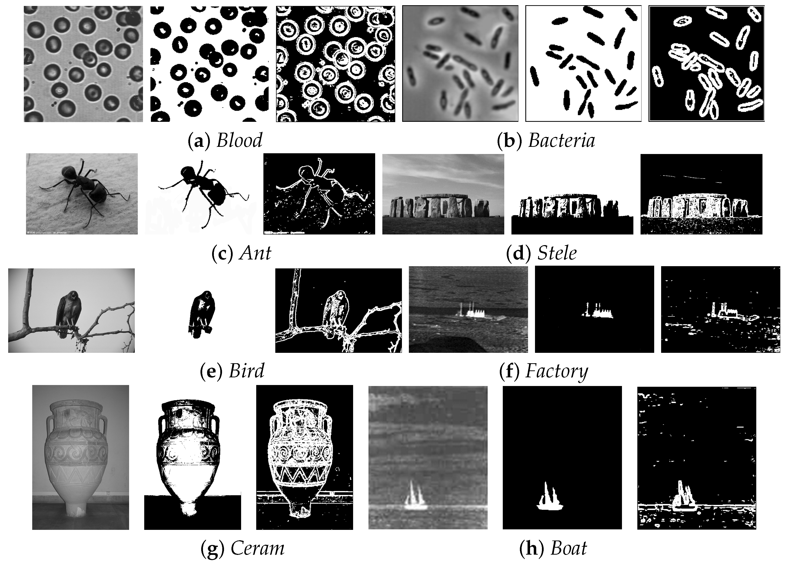
In this section, the proposed method is tested on various images and compared to other thresholding methods, including Kapur’s 1D entropic method (1D KSW), Abutaleb’s 2D approach (2D KSW), Xiao’s GLSC proposition (GLSC KSW), and Xiao’s GLGM proposition (GLGM KSW). These methods are implemented on an Intel Celeron 2.7 GB platform with 1.89 GB RAM using Matlab. The test images are Blood ($272\times 265$), Ant ($331\times 240$), Stele ($545\times 360$), Ceram ($321\times 481$), Bird ($481\times 321$), Bacteria ($178\times 178$), Boat ($256\times 308$), Factory ($185\times 254$), in which some of them are taken from the Berkeley segmentation dataset [23], and some of them are taken from related references. Figure 2 shows all the test images, their ground-truth images, and their local variance images. The ground true images are usually obtained via manual segmentation. In our paper, if the test images are from a dataset, the ground true are also taken from the same dataset, and if the test images are taken from reference, the ground true are also taken from references. The segmentation results obtained by different approaches are shown in Figure 3.

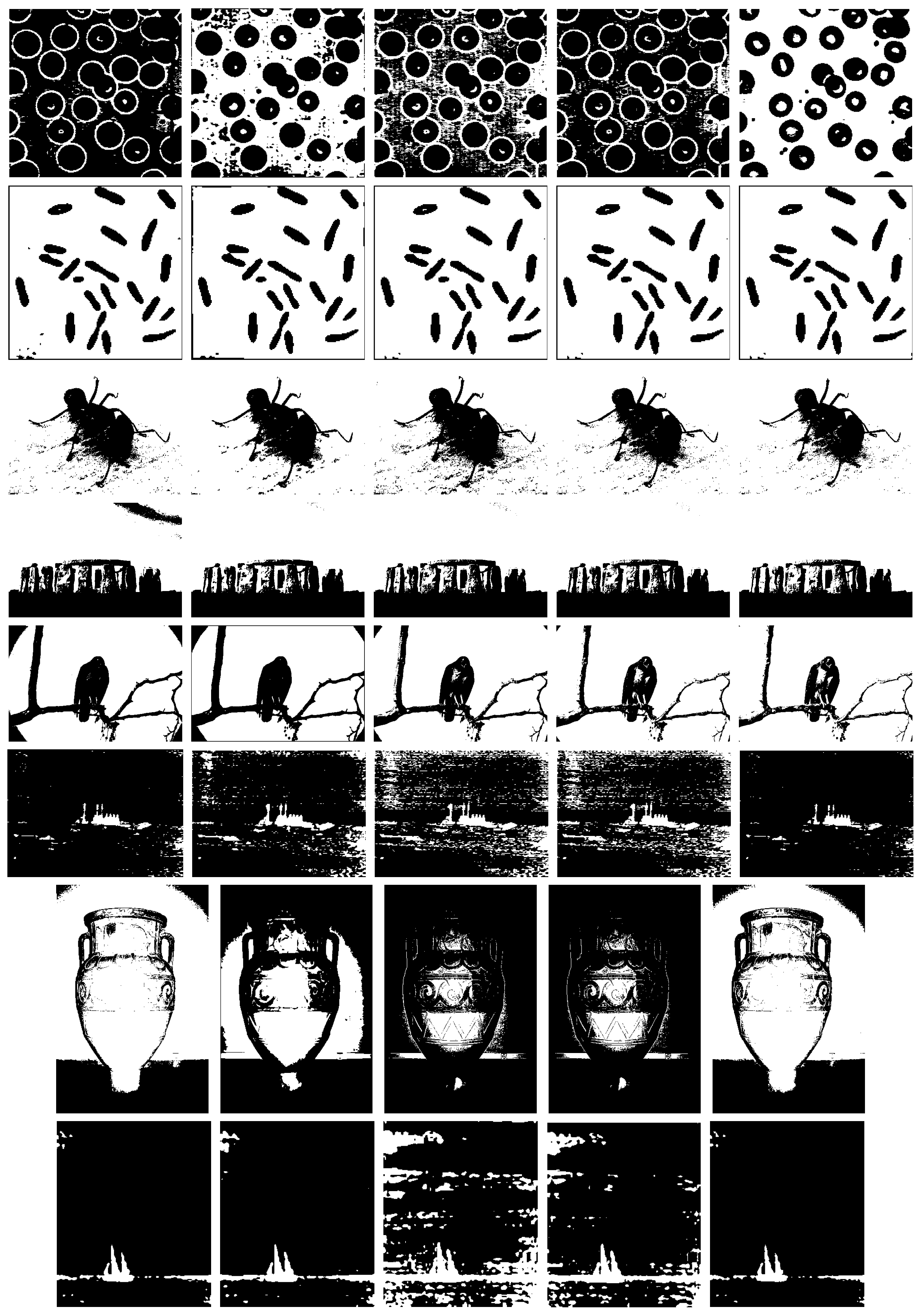
As is shown in Figure 3, for the Blood image, the proposed method gives the best result, and the other four methods cannot produce fully correct segmentation results. The segmentation results of image Ant and the Bacteria by the five methods are similar and acceptable. It can be seen in the segmentation results of the Stele image, except for the resulted image produced by 1D KSW, the other four thresholded images are basically the same. However, upon closer observation, the sky area obtained by our proposed method shows better. The results of the Bird image segmented by the GLSC KSW, GLGM KSW, and our proposed method also have a little difference, but our proposed method gives the better segmentation result. Seen from the results of the Ceram image, the 2D KSW, GLSC KSW, and GLGM KSW methods do not give satisfactory segmentation results, while the other two methods produce acceptable results. For the last two images (Boat and Factory), the proposed method and the 1D KSW yield good threshold results; however, the 2D KSW, GLSC KSW, and GLGM KSW are not suitable.

To evaluate the efficiency and accuracy of the proposed method, the misclassification error (ME) is adopted, which is only limited to the case of bi-level threshold evaluation. The results of ME for each image are used to illustrate the accuracy of the five thresholding methods.

ME is an important index that reflects the percentage of background pixels wrongly assigned to the objects, and conversely, foreground pixels wrongly assigned to the background. For a two-class segmentation, ME [24,25] can be simply formulated as

$$ME=1-\frac{|B_o\cap B_T|+|F_o\cap F_T|}{|B_o|+|F_o|},$$

(13)

where $B_o$ and $F_o$ denote the background and foreground of the original (ground-truth) image, respectively, $B_T$ and $F_T$ are the counterparts in the thresholded images, respectively, and $|.|$ represents the cardinality of a set. Note that the value of ME varies from 0 for a perfectly well classified image to 1 for a completely wrongly classified one. The lower the value of ME, the better the quality of the corresponding thresholded image.

Table 1. Misclassification error (ME) comparison of the referenced thresholding methods.

Image	1D KSW	2D KSW	GLSC KSW	GLGM KSW	Our Method
Blood	0.5120	0.1059	0.3487	0.4655	0.0176
Ant	0.0909	0.0839	0.1175	0.0817	0.0684
Stele	0.0475	0.0069	0.0070	0.0057	0.0053
Ceram	0.1164	0.2786	0.5044	0.5136	0.1100
Bird	0.1501	0.1508	0.0992	0.0802	0.0740
Bacteria	0.0152	0.0128	0.0059	0.0058	0.0057
Boat	0.0145	0.0297	0.2065	0.1063	0.0129
Factory	0.0204	0.0877	0.1730	0.1730	0.0186

shows the results of ME of the thresholded images obtained by the five methods, which makes it clear that the proposed method can extract the objects from the background more completely, compared with the other four methods.

5. Conclusions

In this paper, a new thresholding method is proposed for image segmentation. First, a novel 2D histogram—called GLLV histogram—is constructed by using the gray level information of pixels and the local variance information. Then, optimal threshold values are selected by maximizing the Shannon entropy of objects and background, which are calculated according to the GLLV histogram. In the GLLV histogram, local variance can reflect the edge information of pixels in a neighborhood in a simple way, and thus, the GLLV histogram can effectively incorporate spatial information into the thresholding procedure. Experimental results and comparisons with other typical thresholding methods show that the proposed method is superior to traditional thresholding methods, including a 1D histogram-based thresholding method and several 2D histogram-based thresholding methods reported recently. The proposed method can be considered a promising and viable method in image segmentation.

References

- Shao, J.X.; Dong, D.; Baohua, C.; Han, S. Automatic weld defect detection based on potential defect tracking in real-time radiographic image sequence. NDT & E Int. 2012, 46, 14–21. [Google Scholar]
- Tsneg, Y.H.; Tsai, D.M. Defect detection of uneven brightness in low-contrast images using basis image representation. Pattern Recognit. 2010, 43, 1129–1141. [Google Scholar] [CrossRef]
- Namane, A.; Guessoum, A.; Soubari, E.; Meyrueis, P. CSM neural network for degraded printed character optical recognition. J. Vis. Commun. Image Represent. 2014, 25, 1171–1186. [Google Scholar] [CrossRef]
- Ramírez-Ortegón, M.A.; Ramírez-Ramírez, L.L.; Märgner, V.; Messaoud, I.B.; Cuevas, E.; Rojas, R. An analysis of the transition proportion for binarization in handwritten historical documents. Pattern Recognit. 2014, 47, 2635–2651. [Google Scholar] [CrossRef]
- Gonçalves, H.; Gonçalves, J.A.; Corte-Real, L. HAIRIS: A method for automatic image registration through histogram-based image segmentation. IEEE Trans. Image Process. 2011, 20, 776–789. [Google Scholar] [CrossRef] [PubMed]
- Otsu, N. A threshold selection method from gray-level histogram. IEEE Trans. Syst. Man Cybern. 1979, 9, 62–66. [Google Scholar] [CrossRef]
- Kittler, J.; Illingworth, J. Minimum error thresholding. Pattern Recognit. 1986, 19, 41–47. [Google Scholar] [CrossRef]
- Pun, T. A new method for grey-level picture thresholding using the entropy of the histogram. Signal Process. 1980, 2, 223–227. [Google Scholar] [CrossRef]
- Pun, T. Entropic thresholding: A new approach. Comput. Vis. Graph. Image Process. 1981, 16, 210–239. [Google Scholar] [CrossRef]
- Wong, K.C.; Sahoo, P.K. A gray-level threshold selection method based on maximum entropy principle. IEEE Trans. Syst. Man Cybern. 1989, 19, 866–871. [Google Scholar] [CrossRef]
- Kapur, J.N.; Sahoo, P.K.; Wong, A.K.C. A new method for gray-level picture thresholding using the entropy of the histogram. Comput. Vis. Graph. Image Process. 1985, 29, 273–285. [Google Scholar] [CrossRef]
- Li, C.H.; Lee, C.K. Minimum cross entropy thresholding. Pattern Recognit. 1993, 26, 617–625. [Google Scholar] [CrossRef]
- Abutaleb, A. Automatic thresholding of gray-level pictures using two-dimensional entropy. Comput. Vis. Graph. Image Process. 1989, 47, 22–32. [Google Scholar] [CrossRef]
- Sahoo, P.K.; Arora, G. A thrsholding methd based on two-dimensional Renyi’s entropy. Pattern Recognit. 2004, 37, 1149–1161. [Google Scholar] [CrossRef]
- Liu, J.Z.; Li, W.Q. The automatic threshold of gray 2 level pictures via two 2 dimensional otsu method. Autom. Sin. 1993, 19, 101–105. (In Chinese) [Google Scholar]
- Tang, Y.; Di, Q.; Zhao, L.; Guan, X.; Liu, F. Image thesholding segmentation based on two-dimensional minimum Tsallis cross entropy. Acta Phys. Sin. 2009, 58, 9–15. [Google Scholar]
- Sahoo, P.K.; Arora, G. Image thresholding using two-dimensional Tsallis-Havrda-Charvat entropy. Pattern Recognit. Lett. 2006, 27, 520–528. [Google Scholar] [CrossRef]
- Xiao, Y.; Cao, Z.; Zhang, T. Entropic thresholding based on gray-level spatial correlation histogram. In Proceedings of the 19th International Conference on Pattern Recognition, Tampa, FL, USA, 8–11 December 2008; pp. 1–4. [Google Scholar]
- Yimit, A.; Hagihara, Y.; Miyoshi, T.; Hagihara, Y. 2-D direction histogram based entropic thresholding. Neurocomputing 2013, 120, 287–297. [Google Scholar] [CrossRef]
- Xiao, Y.; Cao, Z.; Yuan, J. Entropic image thresholding based on GLGM histogram. Pattern Recognit. Lett. 2014, 40, 47–55. [Google Scholar] [CrossRef]
- Wang, Z.J.; Sheng, H.Y. An Approach of Grad-based Image Segmentation. Appl. Res. Comput. 2004, 2, 254–258. [Google Scholar]
- De Albuquerque, M.P.; Esquef, I.A.; Mello, A.R.G. Image thresholding using Tsallis entropy. Pattern Recognit. Lett. 2004, 25, 1059–1065. [Google Scholar] [CrossRef]
- Berkely Image Segmentation Dataset. Available online: https://www2.eecs.berkeley.edu/Research/Projects/CS/vision/bsds/ (accessed on 26 April 2017).
- Huang, D.; Wang, C. Optimal multi-level thresholding using a two-stage Otsu optimization appoach. Pattern Recognit. Lett. 2009, 30, 275–284. [Google Scholar] [CrossRef]
- Li, Z.; Liu, C.; Liu, G.; Cheng, Y.; Yang, X.; Zhao, C. A novel statistical image thresholding method. Int. J. Electron. Commun. 2010, 64, 1137–1147. [Google Scholar] [CrossRef]
Figure 1.
Gray level local variance (GLLV) histogram.
Figure 2.
The testing images, their ground-truth images, and their variance images. (a) Blood; (b) Bacteria; (c) Ant; (d) Stele; (e) Bird; (f) Factory; (g) Ceram; (h) Boat.
Figure 3.
Thresholding results of test images using different methods. From left to right, the results are obtained by 1D KSW (Kapur’s 1D entropic method), 2D KSW (Abutaleb’s 2D approach), GLSC KSW (Xiao’s GLSC proposition), GLGM KSW (Xiao’s GLGM proposition), and our approach.