
Criticality and Information Dynamics in Epidemiological Models


1
Centre for Complex Systems, Faculty of Engineering and IT, University of Sydney, Sydney, NSW 2006, Australia
2
Marie Bashir Institute for Infectious Diseases and Biosecurity, University of Sydney, Westmead, NSW 2145, Australia
*
Author to whom correspondence should be addressed.
†
Current address: Department of Evolutionary Biology and Environmental Studies, University of Zurich, Winterthurerstrasse 190, 8057 Zurich, Switzerland.
Entropy 2017, 19(5), 194; https://doi.org/10.3390/e19050194
Submission received: 2 March 2017
/
Revised: 24 April 2017
/
Accepted: 25 April 2017
/
Published: 27 April 2017
(This article belongs to the Special Issue Complexity, Criticality and Computation (C³))
Abstract
:Understanding epidemic dynamics has always been a challenge. As witnessed from the ongoing Zika or the seasonal Influenza epidemics, we still need to improve our analytical methods to better understand and control epidemics. While the emergence of complex sciences in the turn of the millennium have resulted in their implementation in modelling epidemics, there is still a need for improving our understanding of critical dynamics in epidemics. In this study, using agent-based modelling, we simulate a Susceptible-Infected-Susceptible (SIS) epidemic on a homogeneous network. We use transfer entropy and active information storage from information dynamics framework to characterise the critical transition in epidemiological models. Our study shows that both (bias-corrected) transfer entropy and active information storage maximise after the critical threshold ( = 1). This is the first step toward an information dynamics approach to epidemics. Understanding the dynamics around the criticality in epidemiological models can provide us insights about emergent diseases and disease control.
1. Introduction
The mathematical modelling of epidemics dates back to mid-18th century [1], while it was Kermack and McKendrick [2] who studied Susceptible-Infected-Recovered (SIR) model, being the first to use the formal models of epidemics, known generally as compartmental mean-field models [3]. In these models, the population is categorised into distinct groups, depending on their infection status: susceptible individuals are the ones who has never had the infection and can have it upon contact with infected individuals, infected individuals have the infection and can transmit it to the susceptible individuals, and recovered individuals are those have recovered from the infection and are immune since then. This baseline model is captured mathematically by the following set of ordinary differential equations (ODEs):
where is the transmission rate, is the recovery rate, and S, I and R are the proportion of susceptible, infected and recovered individuals respectively. These equations can be further modified to account for various other factors (e.g., pathogen-induced mortality) by the inclusion of more parameters in the ODEs, or they can be adapted to reflect different infectious dynamics (e.g., waning immunity).
Compartmental mean-field models are simplistic: for instance, they do not account for the contact structure in the population, which can influence epidemic dynamics (e.g., [4,5]). However, they were crucial in understanding the epidemic threshold: an epidemic with the dynamics as described in Equations (1)–(3) can invade a population only if the initial fraction of the susceptible population is higher than [2,3,6]. The inverse of this value is called ‘basic reproductive ratio’ () which is defined as “the expected number of secondary cases produced by a typical infected individual during its entire infectious period, in a population consisting of susceptibles only” [7]. An infection will cause an epidemic only if (endemic equilibrium in models with population dynamics) and will die out if (disease-free equilibrium or extinction) [8]. This is rather intuitive: if each individual transmits the disease to less than one other individual on average, the infected individuals will be removed from the population (for instance, due to recovery) faster than they transmit the disease to the susceptible individuals [9]. However, recurring contacts between a typical infective individual and other previously infected individuals may cause to overestimate the mean number of secondary infections, so more exact measures may sometimes be required [10].
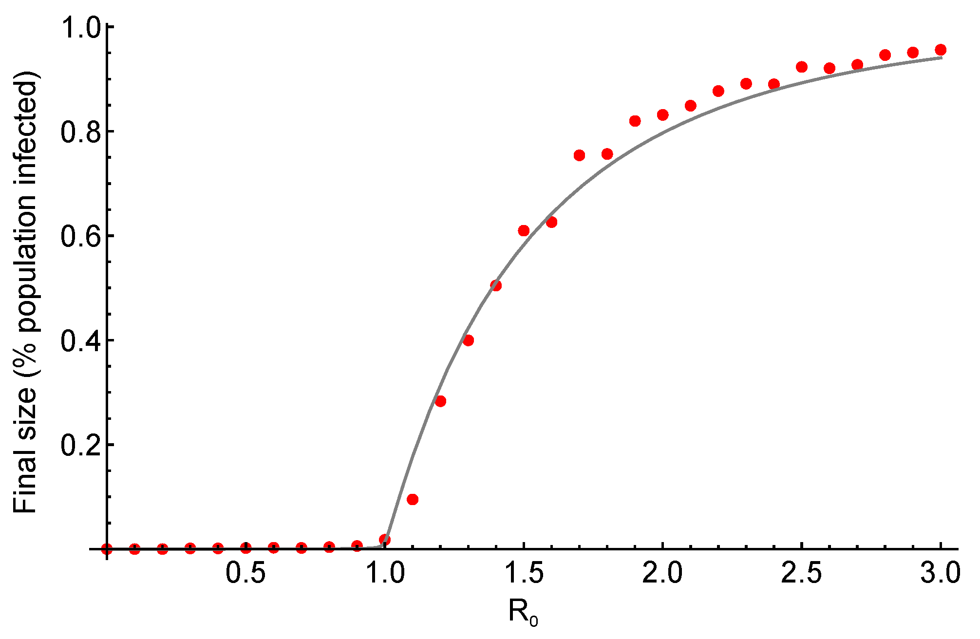
The epidemic threshold is a well-known result in epidemiology, and can be related to the concepts of phase transitions and critical thresholds in statistical physics [11]. A phase transition is “a sharp change in the properties (state) of a substance (system)” that happens when “there is a singularity in the free energy or one of its derivatives” and occurs through changing a control parameter [11,12]. It is observed in various systems, such as fluid or magnetic phase transitions [12]. The phases are distinguished by the order parameter , which is typically zero in one phase and attains a non-zero value in the other [11]. When the control parameter takes the value , known as critical point, the phase transition occurs such that when , while , [11]. For instance, in the case of liquid-gas transition, the difference between the densities of liquid and gas becomes zero as the temperature increases above the critical temperature [12]. Relating back to the analogy in epidemiology, we see that an epidemic occurs only if , as shown in Figure 1. The control parameter, in this case, is , while and the order parameter is the final size of the epidemic (which can alternatively be the density of the infected individuals or prevalence [11]).
The basic reproductive ratio is widely used for modelling, predictions and control of epidemics (see [9] for examples). Furthermore, understanding the dynamics when a pathogen is near the epidemic threshold is crucial. A maladapted pathogen with can cause an epidemic if its exceeds 1 (due to, for instance, mutations or changes in the host population), which is how new pathogens can emerge by crossing the species barrier [13]. From a phase transition point-of-view, Reference [14] have studied the change in epidemiological quantities while approaching the critical point, in order to see if they can be used for anticipating the emergence of criticality and potential elimination of such dynamics. Their results suggest that theoretically, we can predict critical thresholds in epidemics [14], which could be of a substantial value in health care. In practice, one of the challenges lies in pinpointing such critical thresholds in finite-size systems, where a precise identification of phase transitions requires an estimation of the rate of change of the order parameter, often from finite and/or distributed data [15,16].
Information dynamics [17,18,19,20,21] is a recently-developed framework based on information theory [22], which shows promise in characterising phase transitions in dynamical systems. For instance, in studies of the order-chaos phase transitions in random Boolean networks (driven by changes in activity [23] and/or network structure [24]), information storage has been shown to peak just on the ordered side, whereas information transfer was found to maximise on the other (chaotic) side of the critical threshold. Information transfer, from a collection of sources, has also been measured to peak prior to the phase transition in the Ising model, when the critical point is approached from the disordered (high-temperature) side [25]. And similarly, both information storage and transfer were measured to be maximised near the critical state in echo-state networks (a type of recurrent neural network) [26], where such networks are argued to be best placed for general-purpose computation.
Furthermore, one of the features of complex computation is a coherent information structure defined as a pattern appearing in a state-space formed by information-theoretic quantities, such as transfer entropy and active information storage [27]. The “information dynamics” state-space diagrams are known to provide insights which are not immediately visible when the measures are considered in isolation [28]. For example, critical spatiotemporal dynamics of Cellular Automata (CA) were characterised via state-space diagrams formed by transfer entropy and active information storage. These state-space diagrams highlighted how the complex distributed computation carried out by CA interlinks the communication and memory operations [27].
Local information dynamics were also shown to have maxima that relate to the spread of cascading failures in energy networks [29]. We, therefore, expect that this framework will prove to be applicable not only to explaining epidemic dynamics around the critical threshold, but also in developing new predictive methods during emergence of diseases, evolution of pathogens and spillage from zoonotic reservoirs, as well as applications of stochastic epidemiological models to computer virus spreading and other similar scenarios [30].
Here we study the phase transition in a SIS model of epidemics using the information dynamics framework. We model a homogeneous network where a pathogen can spread through contact between the neighbours. Changing the transmissibility of the pathogen between different realisations of the same network while keeping the recovery rate fixed, we use basic reproductive ratio as the control parameter. We track the prevalence of the infection as our order parameter and use the infection status of individuals to calculate the transfer entropy and active information storage.
2. Materials and Methods
2.1. Model Description
We focus on Susceptible-Infected-Susceptible (SIS) dynamics [31] which were originally defined using the following ODE mean-field model:
where is the transmission rate, is the recovery rate.
As described in Section 1 however, such ODE models do not account for contact structure in the population, and so we use the following network model. We simulate a population of individuals, where each is connected to four neighbours (randomly selected from the network), and assume the network is undirected. Susceptible (S) individuals can become infected through contact with their infected (I) neighbours with transmission rate and infected individuals can recover with recovery rate . Each individual has the same rate of transmission and recovery. We scale the transmission rate by c to calculate per contact transmission rate in the event-based simulations. It is a closed population, therefore for the total population . Also, we assume there is no mortality due to infection and N remains constant through the simulations (i.e., we neglect births and deaths in the population). At the beginning of the simulation one random individual gets infected and the epidemiological process is simulated using the Gillespie’s Direct Algorithm [32]. For each parameter set (summarised in Table 1), we ran either 500 replicates or 10 complete runs (i.e., simulations that ran for time steps), depending on whichever is attained first. We binned the continuous time to discrete time steps for our information dynamic analysis and recorded the infectious status of each individual and their four neighbours once in every time step.
2.2. Information Dynamics
Disease spreading could be considered as a computational process by which a population “computes” how far a disease will spread, and what the final states (susceptible or recovered) of the various individuals will be once the disease has run its course. The framework of local information dynamics [17,18,19,20,21] studies how information is intrinsically processed within a system while it is “computing” its new state. Specifically, the information dynamics framework measures how information is stored, transferred and modified within a system during such a computational process. It is a recently-developed framework, based on information theory [22], and involving a well-established quantity for measuring the uncertainty of a random variable X, known as Shannon entropy, which is written as:
where is the probability that X takes the state i. This quantity has been used to derive other measures such as joint entropy, which quantifies uncertainty of joint distribution of random variable X and Y, or mutual information, which is the expression of the amount of information that can be acquired concerning one random variable by observing another [33].
Once we begin to consider how to predict disease spread, we naturally turn to measuring uncertainties and uncertainty reduction using information theory. Information theory has previously been used to study the uncertainty (and conversely, the predictability) of disease spreading dynamics using the permutation entropy of the total number of infections in the population [34]. Another related study analysed the dynamics of an infectious disease spread by formulating the maximum entropy solutions of the SIS and SIR stochastic models, exploiting the advantage offered by the Principle of Maximum Entropy in introducing the minimum additional information beyond the information implied by the constraints on the conserved quantities [35].
Our investigation will focus on measuring information dynamics of an epidemic process within the population, seeking to relate the spread of the disease to information-processing (computational) primitives such as information storage and transfer. Moreover, while these quantities are defined for studying averages over all observations, the corresponding local measures—specific to each sample of a state i of X—can provide us with more suitable tools to study phase transitions in finite-size systems (e.g., [36]).
The information dynamics framework quantifies information transfer, storage and modification, and focusses on their local dynamics at each sample. Information storage is defined as “the amount of information in [an agent’s] past that is relevant to predicting its future” while the local active information storage [19] is the local mutual information between an agent’s next state () and its semi-infinite past expressed as:
The average active information storage is the expectation value over the ensemble:
On the other hand, information transfer is defined via the transfer entropy [37] as the information provided by the source about the destination’s next state in the context of the past of the destination [23], whereas local information transfer from a source Y to a destination X is “the local mutual information between the previous state of the source and the next state of the destination conditioned on the semi-infinite past of the destination”, expressed as:
following [17]. The (average) transfer entropy is the expectation value of the local term over the ensemble:
Transfer entropy was recently analysed on SIS dynamics (generated on brain network structures) in order to investigate information flows on different temporal scales [38].
In order to determine which embedding length k is most suitable for our analysis, we seek to set k so as to maximise the average active information storage, as per the criteria presented in [39]. Importantly though, for this criteria to work we need to maximise the bias-corrected active information storage rather than its raw value. Bias-correction pertains to removing the bias in our estimation of , i.e., the systematic over- or under-estimation of that quantity as compared to the true value. Typically, as a mutual information quantity, will be overestimated from a finite amount of data, particularly when our embedding length k starts to increase the dimensionality of our state space beyond a point that we have adequately sampled. We can estimate this bias by computing the mutual information between surrogate variables with the same distribution as those we originally consider, but without their original temporal relationship to each other [40]. For , one surrogate measurement is made with a shuffled version of the samples (but keeping the samples fixed), and then repeating to produce a population of surrogate measurements. We label the mean of these surrogate measurements , and our effective or bias-corrected active information storage as:
Subtracting out bias using surrogates was proposed earlier for the transfer entropy as the “effective transfer entropy” [41], simply referred to as “bias-corrected transfer entropy” here. Computing the bias-corrected transfer entropy is performed in a similar fashion to : first, surrogates are computed using a shuffled version of the source samples while holding the destination time series fixed (to retain the destination past–next relationship via ), then the mean of the surrogate measurements is computed, before computing the effective or bias-corrected transfer entropy as:
To perform the information dynamics calculations in this study we used the Java Information Dynamics Toolkit (JIDT) [40].
2.3. Measuring Information Dynamics in the SIS Model
We analysed three simulation runs of the SIS model for each parameter combination and required these runs to be at least 14 time steps of length for (as these runs did not have sustained transmission of infection for time steps, 14 being the number of time steps in the third longest run for ).
We used the past and current status of individuals (1 if infected, 0 if susceptible) and that of their neighbours at a given time to determine , , and the vectors for calculations of active information storage and transfer entropy. For instance, if the focal individual is infected and its neighbours are all susceptible at a given time, then was equal to one and was equal to zero for all the neighbours. We then calculated the individual’s local transfer entropy by averaging the pairwise transfer entropy (with a given k) between itself and each of its neighbours. We then averaged the local transfer entropy across the population to determine the average transfer entropy. For active information storage, we calculated the local values for each individual (with a given embedding length k) and averaged these across all the individuals in the population.
To determine the value of k to use, we calculated the bias-corrected active information storage as per Equation (11) for each run, and then averaged the values across runs for each . Subsequently, we calculated the mean for each embedding length k across all values. The bias-corrected active information storage maximises for (Figure 2) and decreases sharply after . As such, applying the criteria discussed above, we select for the embedding length to be used.
3. Results and Discussion
In our simulations, the epidemic dies out without any sustained transmission when , whereas the number of infected individuals reaches an equilibrium when , and the epidemic becomes endemic in the population. We use the mean number of infected individuals throughout the simulation runs to calculate the prevalence for each value, shown in Figure 3.
The average transfer entropy is highest after the critical transition (in the supercritical regime), as shown in Figure 3, reaching its peak at for . This result aligns well with the peak in (collective) transfer entropy slightly in the super-critical regime in the Ising model [25]. In alignment with results in the Ising model, here once the disease dynamics reach criticality, we observe strong effects of one individual on a connected neighbour (measured by the transfer entropy). However, as the dynamics become supercritical, the target neighbour becomes more strongly bound to all of its neighbours collectively, and it becomes more difficult to predict its dynamics based on a single source neighbour alone; as such, the transfer entropy begins to decrease. We also note that the peak in average transfer entropy shifts toward lower values when the embedding time is shorter (not shown).
We see that (raw or non-bias-corrected) average active information storage increases after the critical transition, reaching to its peak at (Figure 3).
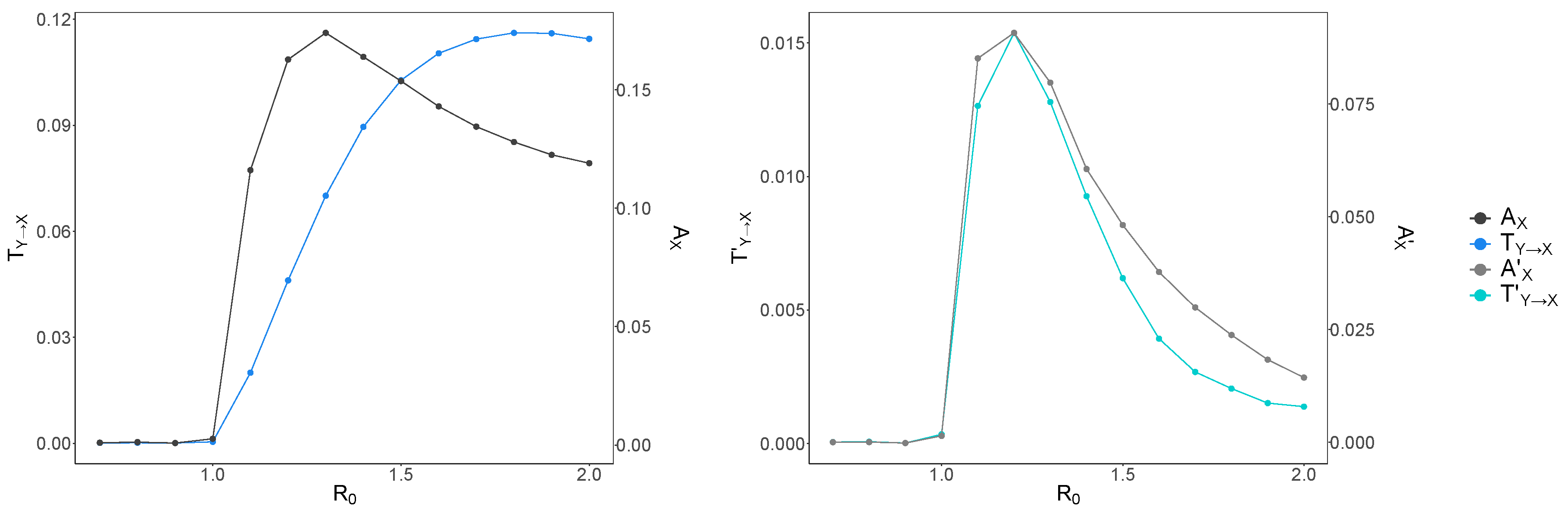
To check whether what we observe for and was a real effect or due to increased bias as the time-series activity increased (with ), we examined the bias-corrected average transfer entropy and average active information storage . This is shown in Figure 4 for embedding length . The bias-corrected average active information storage shows a similar pattern to , however with a sharper peak closer to the phase transition (). This shows that most of what was measured as at larger values was indeed due to increased bias. This is even more striking for the bias-corrected transfer entropy, as we observe a sharp peak at , similar to and much earlier than (). Therefore, these results suggest that once the disease dynamics reach criticality, the state of each individual first exhibits a large amount of self-predictability from its past (information storage). However, as the dynamics become supercritical, the increasingly chaotic nature of the interactions are reflected in the subsequent decrease in self-predictability.
We argue that the transfer entropy captures the extent of the distributed communications of the network-wide computation underlying the epidemic spread, while the active information storage corresponds to its distributed memory. Crucially, the peak of both these information-processing operations (measured with the bias correction) occurs at , rather than the canonical . As mentioned earlier, previous studies of distributed computation and its information-processing operations [23,24,25,27], concluded that the active information storage peaks just on the ordered side, while transfer entropy maximises on the disordered side of the critical threshold. Therefore, in our case, it may be argued that the concurrence of both bias-corrected peaks, as detected by the maximal information-processing “capacity” of the underlying computation, at , indicates an upper bound for the critical threshold in the studied finite-size system.
In the proper thermodynamic limit, as the size of the system goes to infinity, the canonical threshold may well be re-established, but in finite-size systems an additional care may be needed to forecast epidemic spread for intermediate values of the basic reproductive ratio, for instance, as in the presented study. In other words, in finite-size systems one may consider a critical interval rather than an exact critical threshold.
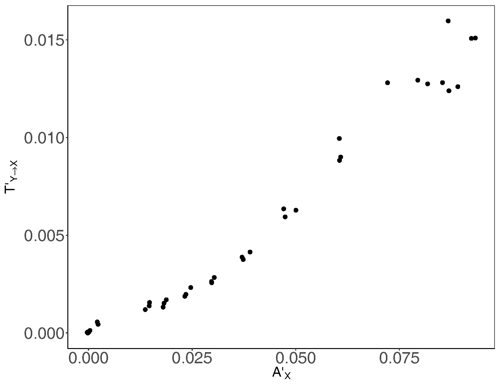
Furthermore, in addition to identifying the peak of information-processing capacity of the underlying computation, which pinpointed an upper bound on the critical basic reproductive ratio , we studied patterns of coherent information structure, via state-space diagrams formed by transfer entropy and active information storage shown in Figure 5. It is evident that both information-processing operations (communications and memory) are tightly interlinked in the underlying computation, suggesting that the studied epidemic process is strongly coherent.
4. Conclusions
In this paper, we studied the criticality in an SIS epidemic within an information dynamics framework. We argued that the transfer entropy captures the extent of the distributed communications of the network-wide computation and showed that it peaks in the super-critical regime. Similarly, we considered the active information storage as a measure of the distributed memory, observing that its maximum is also attained after the canonical critical transition (). To our knowledge, this is the first study to use information dynamics concepts to characterise critical behaviour in epidemics. Crucially, the concurrence of both peaks, which reflect the maximal information-processing capacity of the underlying coherent computation, at , indicates an upper bound for the critical threshold in the studied finite-size system. This supports a conjecture that in finite-size systems a critical interval (rather than an exact critical threshold) may be a relevant notion.
At the time of our study, continuous-time measures of information dynamics were not available. Recently, transfer entropy in continuous-time was formalised with a novel approach [42]. One future avenue for improving our analysis would be using continuous-time measures of information dynamics. Our continuous-time simulation results were binned into discrete time steps in order to conduct an information-dynamic analysis. Therefore, using continuous time measure could reveal novel insights that we missed by the discretisation.
We used a very simplistic network topology in this study, where each individual had the same number of undirected connections that were assigned randomly. However, in real-life, a disease can spread in interaction networks that are heterogeneous in terms of the number of contacts (e.g., [43]) or structured differently (e.g., [5,44]). The heterogeneity and the type of the network can influence not only epidemic dynamics but also disease emergence [4]. Therefore, in future, it would be interesting to expand our analysis to different network topologies and relate the insights from information-dynamic analysis to epidemic dynamics and disease emergence probabilities in these networks.
Finally, we note the wider interest in critical dynamics on complex networks in general. This is particularly the case in complex systems and network approaches to computational neuroscience, where it is conjectured that the brain is in or near a critical state so as to advantageously use maximised computational properties here [26,45,46,47,48]. (Indeed, as noted earlier, SIS dynamics have been used to model dynamics on brain networks [38]). Our results in this paper regarding SIS dynamics continue to add to the quantitative evidence regarding the maximisation of information storage and transfer as intrinsic computational properties at or near critical states, as previously found in a diverse range of dynamics and network structures including the Ising model [25], recurrent neural networks [26], gene regulatory network (GRN) models [23], and regular–small-world–random transitions in structure [24]. In this way, we have provided another important link for epidemic spreading models to complex networks, criticality and information dynamics.
Acknowledgments
Joseph T. Lizier, Mahendra Piraveenan and Mikhail Prokopenko were supported through the Australian Research Council Discovery grant DP160102742, and Joseph T. Lizier was supported through the Australian Research Council DECRA grant DE160100630.
Author Contributions
E.Y.E., Ma.P. and Mi.P. conceived and designed the model; E.Y.E. implemented the model and conducted the simulations; J.T.L. contributed analysis tools; E.Y.E., Ma.P., J.T.L. and Mi.P. analysed the data; E.Y.E., Ma.P., J.T.L., and Mi.P. wrote the paper.
Conflicts of Interest
The authors declare no conflict of interest.
References
- Bernoulli, D. Essai d’une nouvelle analyse de la mortalité causée par la petite vérole et des avantages de l’inoculation pour la prévenir. Hist. Acad. R. Sci. Mém. Math. Phys. 1766, 1–45. (In French) [Google Scholar]
- Kermack, W.O.; McKendrick, A.G. A contribution to the mathematical theory of epidemics. Proc. R. Soc. Lond. A Math. Phys. Eng. Sci. 1927, 115, 700–721. [Google Scholar] [CrossRef]
- Keeling, M.J.; Rohani, P. Modeling Infectious Diseases in Humans and Animals; Princeton University Press: Princeton, NJ, USA, 2008. [Google Scholar]
- Leventhal, G.E.; Hill, A.L.; Nowak, M.A.; Bonhoeffer, S. Evolution and emergence of infectious diseases in theoretical and real-world networks. Nat. Commun. 2015, 6, 6101. [Google Scholar] [CrossRef] [PubMed]
- Bauer, F.; Lizier, J.T. Identifying influential spreaders and efficiently estimating infection numbers in epidemic models: A walk counting approach. Europhys. Lett. 2012, 99, 68007. [Google Scholar] [CrossRef]
- Anderson, R.M.; May, R.M.; Anderson, B. Infectious Diseases of Humans: Dynamics and Control; Oxford University Press: Oxford, UK, 1992; Volume 28. [Google Scholar]
- Heesterbeek, J.; Dietz, K. The concept of Ro in epidemic theory. Stat. Neerl. 1996, 50, 89–110. [Google Scholar] [CrossRef]
- Artalejo, J.; Lopez-Herrero, M. Stochastic epidemic models: New behavioral indicators of the disease spreading. Appl. Math. Model. 2014, 38, 4371–4387. [Google Scholar] [CrossRef]
- Heffernan, J.; Smith, R.; Wahl, L. Perspectives on the basic reproductive ratio. J. R. Soc. Interface 2005, 2, 281–293. [Google Scholar] [CrossRef] [PubMed]
- Artalejo, J.R.; Lopez-Herrero, M.J. On the Exact Measure of Disease Spread in Stochastic Epidemic Models. Bull. Math. Biol. 2013, 75, 1031–1050. [Google Scholar] [CrossRef] [PubMed]
- Pastor-Satorras, R.; Castellano, C.; Van Mieghem, P.; Vespignani, A. Epidemic processes in complex networks. Rev. Mod. Phys. 2015, 87, 925–979. [Google Scholar] [CrossRef]
- Yeomans, J.M. Statistical Mechanics of Phase Transitions; Oxford University Press: Oxford, UK, 1992. [Google Scholar]
- Antia, R.; Regoes, R.R.; Koella, J.C.; Bergstrom, C.T. The role of evolution in the emergence of infectious diseases. Nature 2003, 426, 658–661. [Google Scholar] [CrossRef] [PubMed]
- O’Regan, S.M.; Drake, J.M. Theory of early warning signals of disease emergenceand leading indicators of elimination. Theor. Ecol. 2013, 6, 333–357. [Google Scholar] [CrossRef]
- Wang, X.R.; Lizier, J.T.; Prokopenko, M. Fisher Information at the Edge of Chaos in Random Boolean Networks. Artif. Life 2011, 17, 315–329. [Google Scholar] [CrossRef] [PubMed]
- Prokopenko, M.; Lizier, J.T.; Obst, O.; Wang, X.R. Relating Fisher information to order parameters. Phys. Rev. E 2011, 84, 041116. [Google Scholar] [CrossRef] [PubMed]
- Lizier, J.T.; Prokopenko, M.; Zomaya, A.Y. Local information transfer as a spatiotemporal filter for complex systems. Phys. Rev. E 2008, 77, 026110. [Google Scholar] [CrossRef] [PubMed]
- Lizier, J.T.; Prokopenko, M.; Zomaya, A.Y. Information modification and particle collisions in distributed computation. Chaos 2010, 20, 037109. [Google Scholar] [CrossRef] [PubMed]
- Lizier, J.T.; Prokopenko, M.; Zomaya, A.Y. Local measures of information storage in complex distributed computation. Inf. Sci. 2012, 208, 39–54. [Google Scholar] [CrossRef]
- Lizier, J.T. The Local Information Dynamics of Distributed Computation in Complex Systems; Springer: Berlin/Heidelberg, Germany, 2013. [Google Scholar]
- Lizier, J.T.; Prokopenko, M.; Zomaya, A.Y. A Framework for the Local Information Dynamics of Distributed Computation in Complex Systems. In Guided Self-Organization: Inception; Prokopenko, M., Ed.; Springer: Berlin/Heidelberg, Germany, 2014; Volume 9, pp. 115–158. [Google Scholar]
- Shannon, C.E. A mathematical theory of communication. Bell Syst. Tech. J. 1948, 27, 379–423. [Google Scholar] [CrossRef]
- Lizier, J.T.; Prokopenko, M.; Zomaya, A.Y. The Information Dynamics of Phase Transitions in Random Boolean Networks. Artif. Life 2008, 11, 374–381. [Google Scholar]
- Lizier, J.T.; Pritam, S.; Prokopenko, M. Information dynamics in small-world Boolean networks. Artif. Life 2011, 17, 293–314. [Google Scholar] [CrossRef] [PubMed]
- Barnett, L.; Harré, M.; Lizier, J.; Seth, A.K.; Bossomaier, T. Information Flow in a Kinetic Ising Model Peaks in the Disordered Phase. Phys. Rev. Lett. 2013, 111, 177203. [Google Scholar] [CrossRef] [PubMed]
- Boedecker, J.; Obst, O.; Lizier, J.T.; Mayer, N.M.; Asada, M. Information processing in echo state networks at the edge of chaos. Theory Biosci. 2012, 131, 205–213. [Google Scholar] [CrossRef] [PubMed]
- Lizier, J.T.; Prokopenko, M.; Zomaya, A.Y. Coherent information structure in complex computation. Theory Biosci. 2012, 131, 193–203. [Google Scholar] [CrossRef] [PubMed]
- Cliff, O.M.; Lizier, J.T.; Wang, P.; Wang, X.R.; Obst, O.; Prokopenko, M. Quantifying Long-Range Interactions and Coherent Structure in Multi-Agent Dynamics. Artif. Life 2017, 23, 34–57. [Google Scholar] [CrossRef] [PubMed]
- Lizier, J.T.; Prokopenko, M.; Cornforth, D.J. The information dynamics of cascading failures in energy networks. In Proceedings of the European Conference on Complex Systems (ECCS), Warwick, UK, 21–25 September 2009; p. 54. [Google Scholar]
- Amador, J.; Artalejo, J.R. Stochastic modeling of computer virus spreading with warning signals. J. Frankl. Inst. 2013, 350, 1112–1138. [Google Scholar] [CrossRef]
- Anderson, R.M.; May, R.M. Infectious Diseases of Humans; Oxford University Press: Oxford, UK, 1991; Volume 1. [Google Scholar]
- Gillespie, D.T. Exact stochastic simulation of coupled chemical reactions. J. Phys. Chem. 1977, 81, 2340–2361. [Google Scholar] [CrossRef]
- Cover, T.M.; Thomas, J.A. Elements of Information Theory; Wiley: New York, NY, USA, 1991. [Google Scholar]
- Scarpino, S.V.; Petri, G. On the predictability of infectious disease outbreaks. arXiv, 2017; arXiv:1703.07317. [Google Scholar]
- Artalejo, J.; Lopez-Herrero, M. The SIS and SIR stochastic epidemic models: A maximum entropy approach. Theor. Popul. Biol. 2011, 80, 256–264. [Google Scholar] [CrossRef] [PubMed]
- Lizier, J.T. Measuring the Dynamics of Information Processing on a Local Scale in Time and Space. In Directed Information Measures in Neuroscience; Wibral, M., Vicente, R., Lizier, J.T., Eds.; Understanding Complex Systems; Springer: Berlin/Heidelberg, Germany, 2014; pp. 161–193. [Google Scholar]
- Schreiber, T. Measuring Information Transfer. Phys. Rev. Lett. 2000, 85, 461–464. [Google Scholar] [CrossRef] [PubMed]
- Meier, J.; Zhou, X.; Hillebrand, A.; Tewarie, P.; Stam, C.J.; Mieghem, P.V. The Epidemic Spreading Model and the Direction of Information Flow in Brain Networks. NeuroImage 2017, 152, 639–646. [Google Scholar] [CrossRef] [PubMed]
- Garland, J.; James, R.G.; Bradley, E. Leveraging information storage to select forecast-optimal parameters for delay-coordinate reconstructions. Phys. Rev. E 2016, 93, 022221. [Google Scholar] [CrossRef] [PubMed]
- Lizier, J.T. JIDT: An Information-Theoretic Toolkit for Studying the Dynamics of Complex Systems. arXiv, 2014; arXiv:1408.3270. [Google Scholar]
- Marschinski, R.; Kantz, H. Analysing the information flow between financial time series. Eur. Phys. J. B 2002, 30, 275–281. [Google Scholar] [CrossRef]
- Spinney, R.E.; Prokopenko, M.; Lizier, J.T. Transfer entropy in continuous time, with applications to jump and neural spiking processes. Phys. Rev. E 2017, 95, 032319. [Google Scholar] [CrossRef] [PubMed]
- Lloyd-Smith, J.O.; Schreiber, S.J.; Kopp, P.E.; Getz, W.M. Superspreading and the effect of individual variation on disease emergence. Nature 2005, 438, 355–359. [Google Scholar] [CrossRef] [PubMed]
- Schneeberger, A.; Mercer, C.H.; Gregson, S.A.; Ferguson, N.M.; Nyamukapa, C.A.; Anderson, R.M.; Johnson, A.M.; Garnett, G.P. Scale-free networks and sexually transmitted diseases: A description of observed patterns of sexual contacts in Britain and Zimbabwe. Sex. Transm. Dis. 2004, 31, 380–387. [Google Scholar] [CrossRef] [PubMed]
- Beggs, J.M.; Plenz, D. Neuronal avalanches in neocortical circuits. J. Neurosci. 2003, 23, 11167–11177. [Google Scholar] [PubMed]
- Priesemann, V.; Munk, M.; Wibral, M. Subsampling effects in neuronal avalanche distributions recorded in vivo. BMC Neurosci. 2009, 10, 40. [Google Scholar] [CrossRef] [PubMed]
- Priesemann, V.; Wibral, M.; Valderrama, M.; Pröpper, R.; Le Van Quyen, M.; Geisel, T.; Triesch, J.; Nikolić, D.; Munk, M.H.J. Spike avalanches in vivo suggest a driven, slightly subcritical brain state. Front. Syst. Neurosci. 2014, 8, 108. [Google Scholar] [CrossRef] [PubMed]
- Rubinov, M.; Sporns, O.; Thivierge, J.P.; Breakspear, M. Neurobiologically Realistic Determinants of Self-Organized Criticality in Networks of Spiking Neurons. PLoS Comput. Biol. 2011, 7, e1002038. [Google Scholar] [CrossRef] [PubMed]
Figure 1.
Epidemic phase transition. Final size of an epidemic as a function of its basic reproductive ratio , for a susceptible-infected-recovered (SIR) model with a homogeneous network structure, with a number of connections (k) of 4 for each individual. Transmission rate varies between 0 and 3 with recovery rate , resulting in ranging between 0 and 3. The line depicts the analytical results whereas the red dots show the results from stochastic simulations with a population size of . The epidemic does not occur for , whereas the final size increases as a function of for values higher than 1. The analytical results and the simulations are in good agreement.

Figure 2.
Bias-corrected active information storage in our simulations as a function of embedding length k. was calculated and then averaged for all three replicates for each . The mean value (shown in y-axis) was then determined for each k (shown in x-axis) across the values. The difference increases as the k increases, maximising at , and decreasing subsequently.
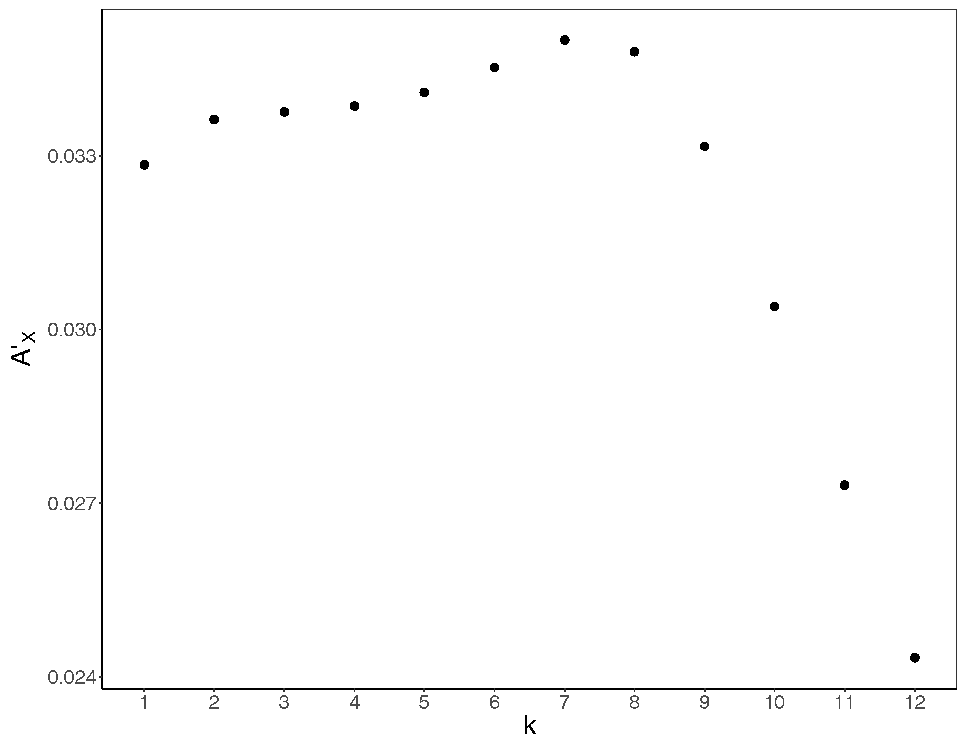
Figure 3.
Raw average transfer entropy and average active information storage versus . Transfer entropy (left) calculated by averaging local transfer entropy for each individual across the network and active information storage (right) calculated by averaging local active information storage for each individual across the network. For both measures, the embedding time is . The average transfer entropy () is shown in blue, the average active information storage () is shown in gray, and prevalence is shown in red (note the different y-axes). is shown on the x-axis. After the critical transition both and increase and reach to a peak (at and , respectively), and subsequently lower down.
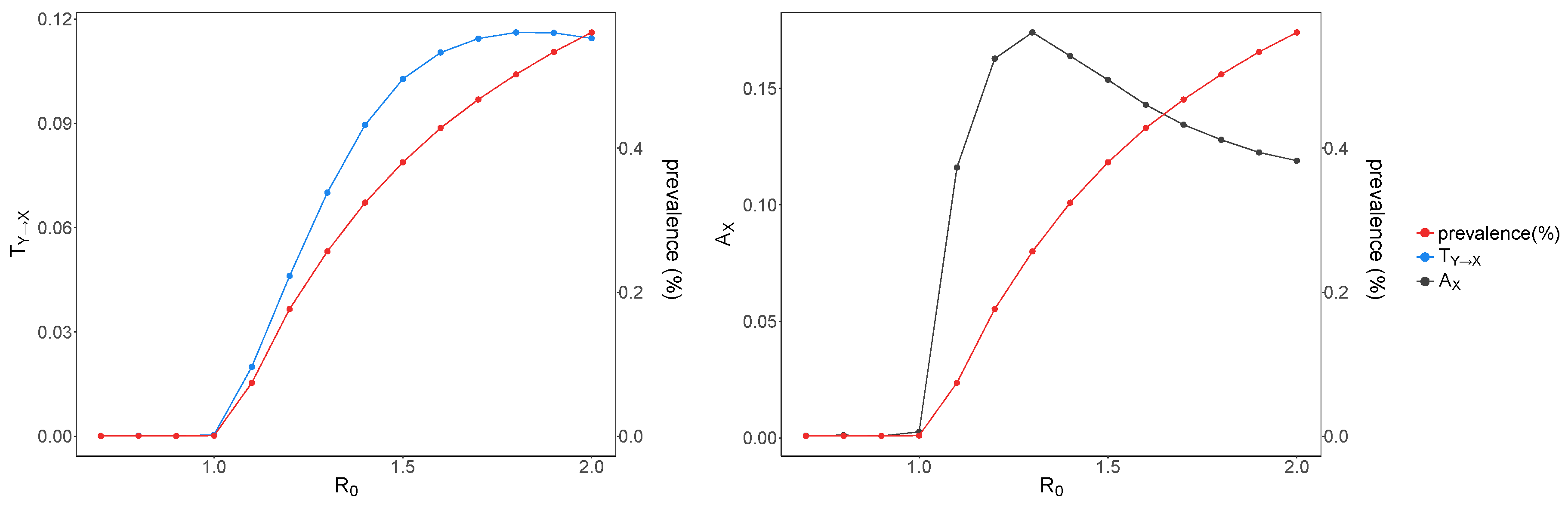
Figure 4.
Raw and bias-corrected average transfer entropy and average active information storage versus . Raw average transfer entropy and average active information storage are shown in dark blue and black, respectively (left panel); bias-corrected average transfer entropy and average active information storage are shown in light blue and gray, respectively (right panel). Note the different y-axes for both graphs. is shown on the x-axis. Both and increase and reach a peak right after the critical transition, and subsequently decrease. also increases at the same value () as and plummets thereafter, whereas reaches its highest value later, at

Figure 5.
Bias-corrected average transfer entropy versus bias-corrected average active information storage . Bias-corrected transfer entropy (shown in the y-axis) and average active information storage (shown in the x-axis) are calculated separately for three replicates.
Figure 5.
Bias-corrected average transfer entropy versus bias-corrected average active information storage . Bias-corrected transfer entropy (shown in the y-axis) and average active information storage (shown in the x-axis) are calculated separately for three replicates.

Table 1.
Simulation parameters.
| Parameter | Value |
|---|---|
| Time steps (t) | |
| Population size (N) | |
| Number of contacts | 4 |
| Transmission rate () | 0.7–2.0 (with step size 0.1) |
| Coefficient for per contact transmission rate (c) | 0.33 |
| Recovery rate () | 1.0 |
© 2017 by the authors. Licensee MDPI, Basel, Switzerland. This article is an open access article distributed under the terms and conditions of the Creative Commons Attribution (CC BY) license (http://creativecommons.org/licenses/by/4.0/).
Share and Cite
MDPI and ACS Style
Erten, E.Y.; Lizier, J.T.; Piraveenan, M.; Prokopenko, M. Criticality and Information Dynamics in Epidemiological Models. Entropy 2017, 19, 194. https://doi.org/10.3390/e19050194
AMA Style
Erten EY, Lizier JT, Piraveenan M, Prokopenko M. Criticality and Information Dynamics in Epidemiological Models. Entropy. 2017; 19(5):194. https://doi.org/10.3390/e19050194
Chicago/Turabian StyleErten, E. Yagmur, Joseph T. Lizier, Mahendra Piraveenan, and Mikhail Prokopenko. 2017. "Criticality and Information Dynamics in Epidemiological Models" Entropy 19, no. 5: 194. https://doi.org/10.3390/e19050194
Note that from the first issue of 2016, this journal uses article numbers instead of page numbers. See further details here.