
A New Kind of Permutation Entropy Used to Classify Sleep Stages from Invisible EEG Microstructure

Institute of Mathematics, University of Greifswald, 17487 Greifswald, Germany
Entropy 2017, 19(5), 197; https://doi.org/10.3390/e19050197
Submission received: 31 March 2017
/
Revised: 21 April 2017
/
Accepted: 26 April 2017
/
Published: 28 April 2017
(This article belongs to the Special Issue Entropy and Sleep Disorders)
Abstract
:Permutation entropy and order patterns in an EEG signal have been applied by several authors to study sleep, anesthesia, and epileptic absences. Here, we discuss a new version of permutation entropy, which is interpreted as distance to white noise. It has a scale similar to the well-known distributions and can be supported by a statistical model. Critical values for significance are provided. Distance to white noise is used as a parameter which measures depth of sleep, where the vigilant awake state of the human EEG is interpreted as “almost white noise”. Classification of sleep stages from EEG data usually relies on delta waves and graphic elements, which can be seen on a macroscale of several seconds. The distance to white noise can anticipate such emerging waves before they become apparent, evaluating invisible tendencies of variations within 40 milliseconds. Data segments of 30 s of high-resolution EEG provide a reliable classification. Application to the diagnosis of sleep disorders is indicated.
1. Introduction
Modern sensor technology makes it possible to monitor vital signs continuously in everyday life, with high precision and without causing much discomfort. This will lead to very personalized, powerful and preventive medical treatment. Sleep medicine is one of the fields where such development is already apparent. While the technical basis is now available, automatic evaluation of the big data series is lagging behind. Classical methods of time series analysis usually require clean data, and preprocessing routines can easily remove information. New methods have to be developed and tested.
Use of order patterns in time series is such a new methodology. Permutation entropy, introduced in [1], has been applied not only to geophysical, financial and machine data but also in biomedical context [2,3,4,5,6]. Here, we are concerned with EEG (electroencephalographic) sleep data only, to which permutation entropy was applied by Ouyang et al. [7], Kuo and Liang [8], Nicolaou and Georgiou [9], and others. We shall introduce a new version of permutation entropy that can be supported by a statistical model which allows for calculating significance, and show how the settings of parameters can be optimized to recognize sleep stages from short time series of a single EEG channel. The presented methodology can be used for other medical applications, such as (see [6,10] for further references):
- Monitoring depth of anesthesia, cf. [15];
- Detecting sleepiness of drivers or workers which may lead to accidents.
In the next section, we define mathematical concepts and compare the new version of permutation entropy with the usual one. A statistical discussion of significance limits for permutation entropy seems to appear here for the first time. In Section 3, we apply our method to a classical database of sleep medicine by Terzano et al. [16], which is available on physionet [17]. The sleep stages annotated by experts apparently coincide with the entropy that is measured on a continuous scale. While the annotation was done by medical doctors on the basis of multichannel data, we use only one EEG channel, and no preprocessing or special treatment of the data, just the simple entropy formula. Segments of 30 s do suffice to evaluate accurately the depth of sleep. While the experts study graphic elements on a scale of several seconds, like delta waves, as recommended by the official guidelines [18], our method analyses the invisible microstructure in high-resolution measurements. EEG data were recorded with 512 Hz, and patterns of length between 4 and 40 ms were studied. In Section 4, we explain how we found optimal parameters, and Section 5 summarizes our main points.
2. Distance to White Noise—A New Version of Permutation Entropy
We consider a time series with T values, denoted In our application, the typical length T will vary between 500 and 20,000. Any three consecutive values can form one of the six order patterns, or permutations, shown in Figure 1. We can also consider three values with a time distance We say the points represent pattern 231, for instance, if In the context of EEG data, ties are very rare. They can be counted as < and will be neglected in the present study. The initial time point t runs from 1 to The delay parameter d can vary between 1 and and has the same meaning as in classical autocorrelation. Usually, consecutive values are considered for permutation entropy, and there are patterns. In this paper, however, we focus on the case for the following reasons:
- we want to keep things simple;
- for we understand the meaning of each pattern;
- results for are good when we consider various delay parameters So far, most authors consider only and different
It should also be mentioned that the statistics of order pattern frequencies are excellent, even for short time series like when we have only six patterns. For for instance, we have patterns and need a very long time series to estimate all of those pattern frequencies. Permutation entropy will still work since it is an average over all patterns. Here, we prefer the simple setting. Let us explain how frequencies are estimated for a pattern We count the number of all appearances of the pattern and divide by the number of places where the pattern can occur:
To understand the method, consider the short time series shown in Figure 2. The table collects the frequencies. As a result, we have and , and could draw this as a kind of autocorrelation function.
Frequencies of single patterns have been studied by several authors [4]. For statistical reasons, we prefer to study only certain sums and differences of pattern frequencies [20,21]. The permutation entropy is the Shannon entropy of the distribution of all patterns. It is defined for the set of all patterns of length m [1]. For our case the sum involves only the six terms indicated in Figure 1. However, the delay parameter d can vary again between 1 and so that permutation entropy also becomes a kind of autocorrelation function:
Entropy as a measure of disorder is a basic concept in physics. Permutation entropy was introduced as complexity measure for time series. H assumes its smallest value zero for a monotone series, and its maximum for white noise, where there is no dependence among the values. White noise means that all possible permutations appear with the same probability . Here, we use a new version of permutation entropy, called ”distance to white noise” and defined for as
We just take the squared Euclidean distance of the observed pattern frequencies from the uniform pattern frequencies in the space of all pattern distributions. Thus, the smallest value of is zero and means complete independence of values. Large means much dependence among the values of the time series. This is easy to understand, and we cannot become confused by terms like “complexity”, “chaos”, and “disorder”. The sum in Equation (3), as well as in Equation (2), contains terms, which means six terms for The equality on the right side of Equation (3) follows from
There are several reasons to call a version of permutation entropy:
- Equation (3) says that we get from H by replacing with the simpler function and adding a constant so that the minimum is zero—not a big change!
- Up to a linear transformation, is the quadratic Taylor approximation of H at white noise ([19], see below for ).
- For a discrete probability space with probabilities the quantity is called Renyi entropy of order 2, or correlation entropy [22], and
- is called Tsallis entropy of order 2 or Kendall information content [23].
For the case of two probabilities p and (length 2 patterns 12 and 21), Figure 3 shows the functions and They do not differ much, and agree asymptotically at the point The same holds for the six probabilities of patterns of order 3. At the point for all which corresponds to white noise, it can be shown that is the quadratic Taylor approximation of H [19]. Note that EEG data, compared to other time series like ECG (electrocardiogram), are very erratic, close to white noise so that H and will lead to similar results. This will be demonstrated in Figure 10.
It turns out that has better statistical properties than In [19], it was shown that can be separated into different components according to an equation
which allows a more detailed study with a kind of ANOVA method. For EEG data, only the component is important and will be discussed below.
We need to know the statistics of permutation entropy in order to check whether certain extreme values of H are mere coincidence or really indicate a certain effect: good order or large disorder. Although a few hundred papers deal with permutation entropy, this statistical aspect seems to be discussed here for the first time.
For statistical inference, we always need a null model. In our case, the null hypothesis is that the data are white noise: completely independently chosen random numbers from the same distribution. The type of distribution does not matter for ordinal patterns. We can take the uniform distribution on In a computer simulation, we now take a large number say 10 million, time series of length all made of independent random numbers. We determine the permutation entropy for each sample series, getting N possible values These N values vary near the maximum value , which is the theoretical value of permutation entropy of length 3 patterns for white noise. In each sample series, the value is somewhat smaller, however.
It is reasonable to consider to get a standard scale with maximum value 1. Figure 4 shows the density of all N sample series. We see that all standardized H-values vary between 0.99 and the maximum value 1. The conclusion is that when we observe a time series of length in practice, and is less than 0.99, we can be sure that this is not a random deviation from white noise! Even 0.995 would be a significant observation, since the tail probability or p-value of 0.995 shown in the lower panel of Figure 4 is about This means that only of our 10 million simulations of white noise gave a standardized H value below 0.995. The value 0.99 is more significant, however, since only 100 samples gave a still smaller which corresponds to a p-value of
The tail probability of in Figure 4 is almost a linear function in semilogarithmic representation, so it is easy to approximate numerically. There are two problems, however. First, the scale between 0.99 and 1 is not very intuitive. It can lead to confusion between quantile values of the H-statistics and the p-values themselves. Second, and worse, the dependence on T has not been considered. It is clear that the simulation will vary more when we have smaller that is, shorter time series. The mathematical formula for this dependence is not obvious.
On the right-hand side of Figure 4, was simulated for the 10 million sample series. Its distribution very much resembles a distribution known from classical statistics. In contrast to extreme values are on the right. The quantiles are spread over a wider range, as seen in the lower panel and in Table 1. Even more importantly, we have drawn instead of Since distance to white noise is a kind of variance, it can be shown to scale with and the curves of almost coincide for T larger 1000. Thus, the critical values of in Table 1 are almost universal while the critical values of are valid for only. To give just one example, the value 4.68 for the 0.01% threshhold of is 4.67 for and 4.69 for while the -quantile 0.9921 of standardized H will change to 0.9843 and 0.9961, respectively. Still more extreme quantiles are harder to simulate and less stable.
To conclude our statistical discussion, let us note that this is just a beginning. More modelling is needed. The white noise hypothesis is not so exciting and would not make sense for heart or respiration data. For EEG data and, in particular, for sleep stages; however, white noise is a reasonable null hypothesis, as we shall see below.
3. as a Measure of Sleep Depth
We briefly explain the basic idea for our classification of sleep stages. The brain of a healthy awake adult fulfils a large variety of functions, and each EEG channel covers the activity of millions of neurons in the cortex. Thus, normally, the signal will be almost white noise. With the onset of sleep, neuronal activity will become weaker and less diverse, and global rhythms are taking over. Global phenomena become visible for a human observer of the data as delta waves, sleep spindles, K-complexes, as described in the official guidelines for sleep scoring [18]. However, long before global phenomena become visible, they manifest themselves in statistical properties of the fine structure of high-resolution data. For our application, the main change is an increase of the frequency of patterns 123 and 321, compared to the other patterns of Figure 1.
In other words, the number of local minima and maxima will decrease. Since a change of standardized H from 1 to 0.99 is already highly significant, such a statistical tendency can be swiftly determined with permutation entropy. Using the language of Fourier analysis, we would state that high frequencies become weaker. However, the idea of brain signal as a composition of sine waves is not quite correct. Such waves may develop only partially, for less than a quarter than a wavelength. In such cases, they are detected by permutation entropy before the frequency spectrum shows any changes. Moreover, order pattern statistics is much more stable and less susceptible to data artefacts than the Fourier frequency statistics.
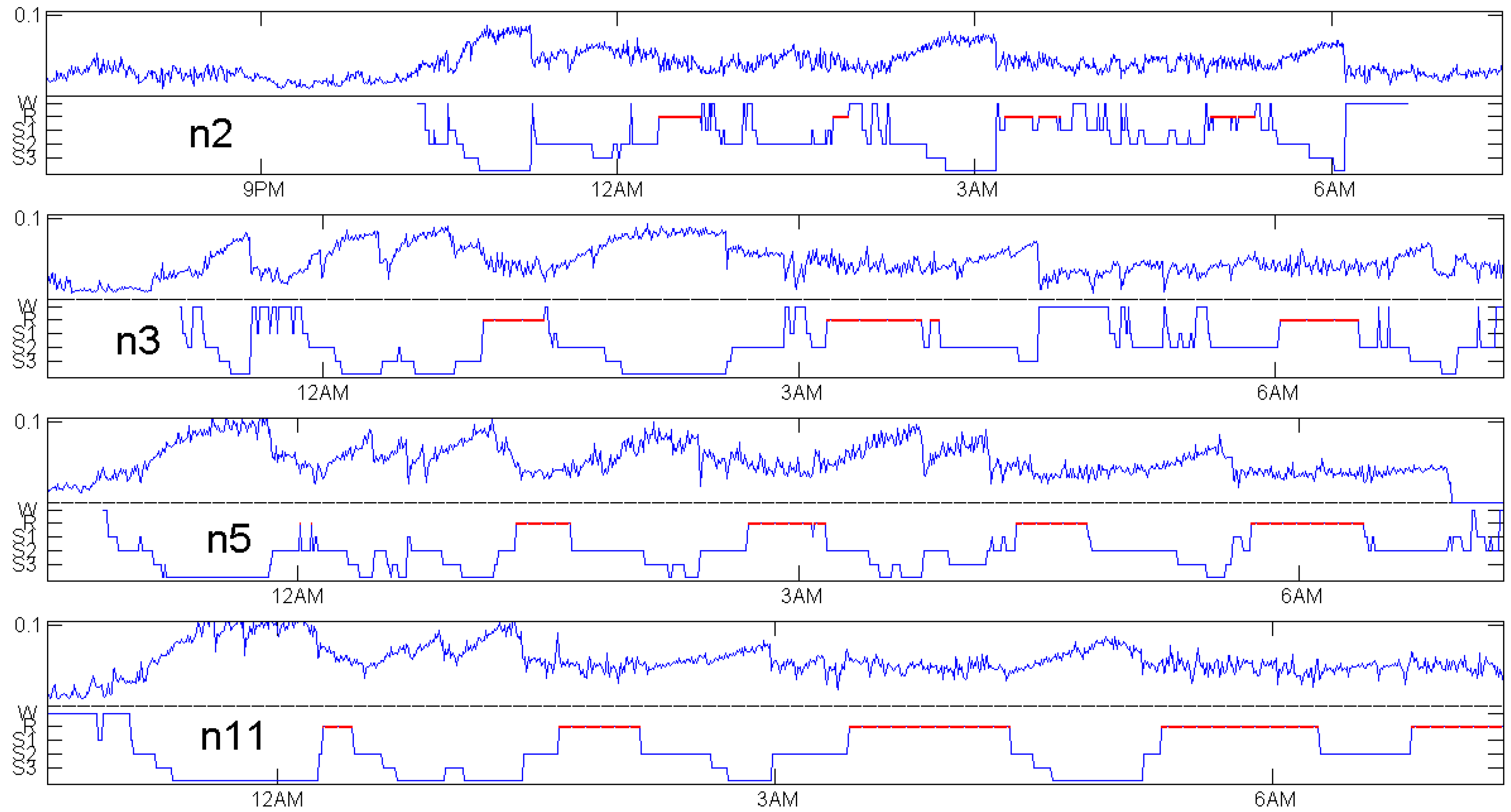
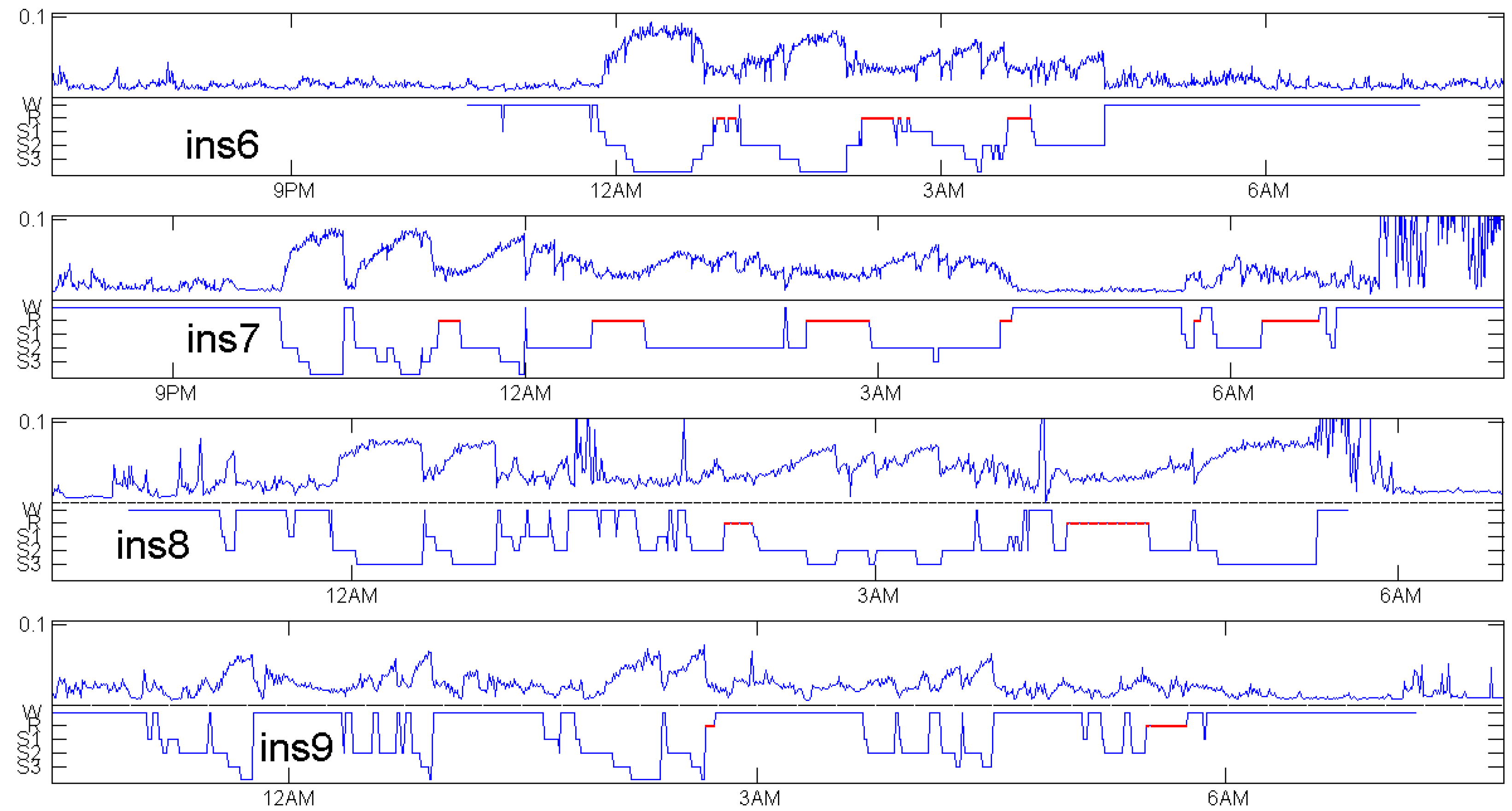
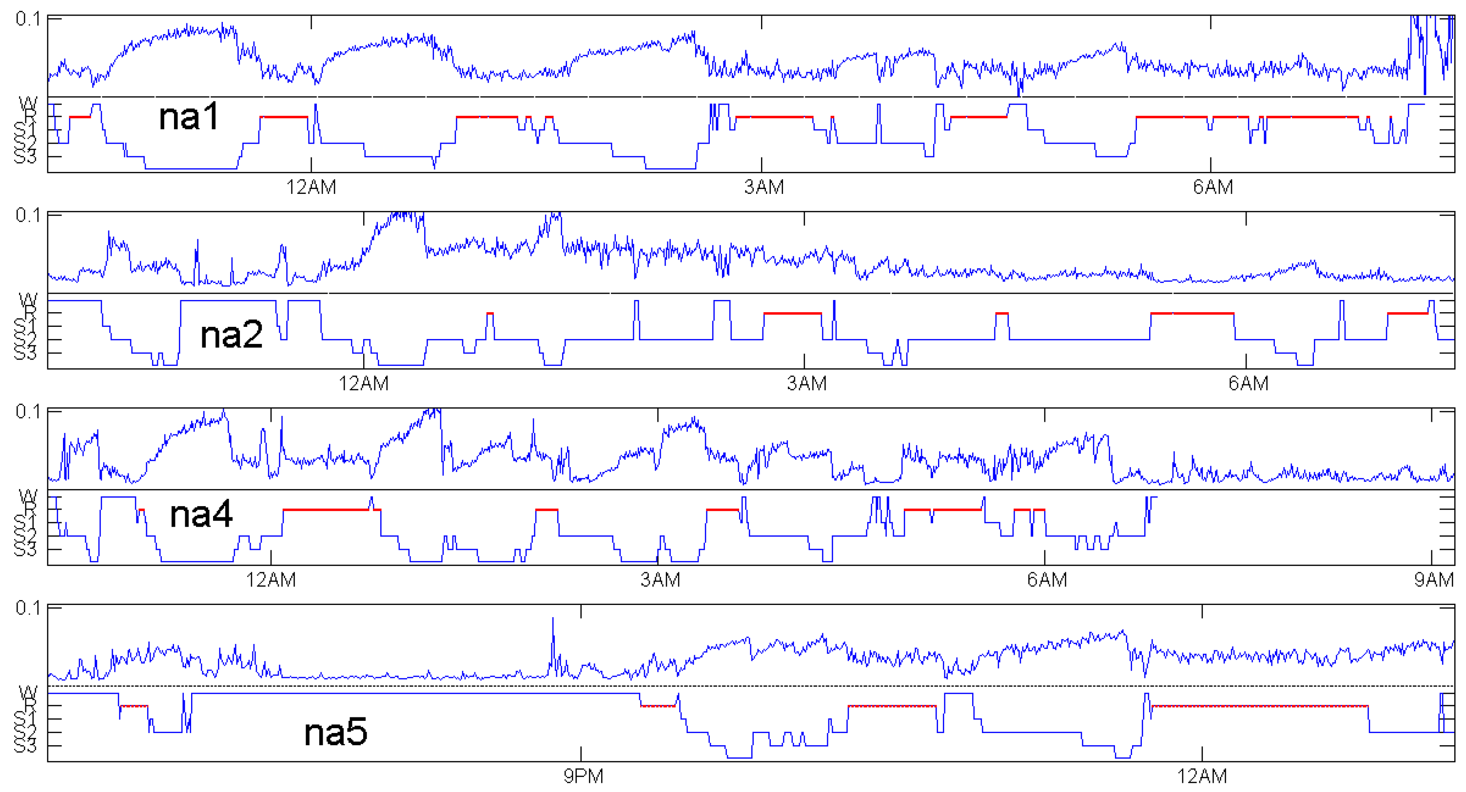
The deeper the sleep, the more our EEG signal will deviate from white noise. Thus, should be a good measure for sleep depth. Figure 5 shows how well this idea works. We have chosen the classical CAP sleep database of Terzano et al. [16] for different reasons: it is freely available at physionet [17]. It contains a number of EEG measurements taken with sample rate 512 Hz while many other datasets contain 128 Hz measurements or low-pass filtered signals. The data quality is good and expert sleep annotation files are provided, still including sleep stage S4, which was later abandoned [18].
For four healthy subjects, Figure 5 shows the expert annotation as a step function on the lower part and as a noisy function on the upper part of the respective panel. It turns out that we almost have mirror symmetry. Whenever the sleep stage increases, increases, and vice versa. The calculation of was done with the data as they were provided, without any preprocessing or selection of “clean segments”. Non-overlapping windows of 30 s in length were used to calculate each value.
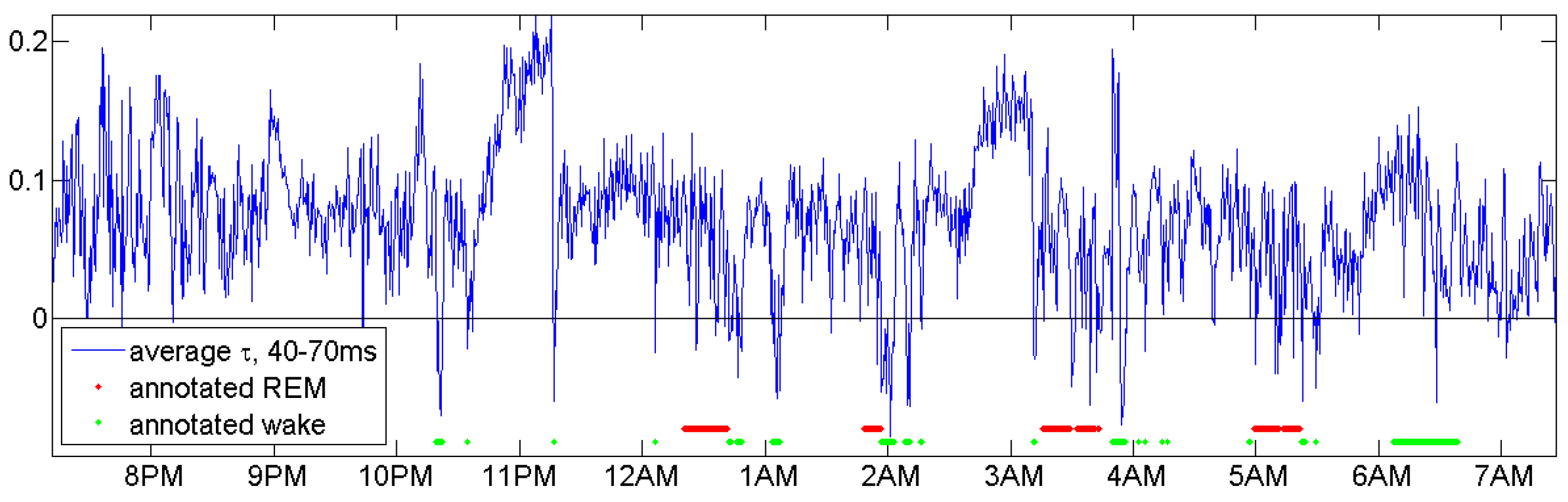
REM (rapid eye movement) phases, indicated by red lines in every annotation of Figure 5, are not considered here. Figure 6 below shows that with modified delays, a function related with and defined in Equation (5) below can indicate REM phases, but does not classify them accurately. We should admit that this is not a systematic study, which would need tight cooperation with medical experts and could be better done with recent measurements. Moreover, if our primary interest was accurate classification, we had to use the whole power of multivariate datasets. Here, the challenge was to get maximum information from a single EEG channel.
The choice of patients for Figure 5 was based on availability of an EEG channel with 512 Hz frequency in the data, not at all on the quality of the coincidence. There were only four healthy controls with a 512 Hz EEG channel. Figure 7, Figure 8 and Figure 9 show patients with insomnia, narcolepsy and nocturnal frontal lobe epilepsy with high-resolution EEG channel from the CAP sleep database of Terzano et al. [16] available at physionet [17]. The coincidence of annotation and was always excellent, though there were more artefacts. The standard EEG channel was Fp2–F4. On three occasions, another channel was provided, and gave similar results.
For the healthy subjects in Figure 5, maximum values of do not differ much: they are around 0.1. We do not know whether it makes sense to compare sleep depth of different persons just by Maybe individual factors do influence We even had no data to check changes of when one subject is measured repeatedly. We think will not depend much on measurement details, but this was not verified. In Figure 7, showing patients with insomnia, the overall level of is much lower than for the controls in Figure 5. This indicates that can also detect certain sleep disorders, by taking the average and grouped box plots over several hours. In a similar way, average can be used to compare the sleep of one subject in several nights or under different conditions. There are numerous ways to exploit the permutation entropy.
Actually, it does not matter whether we take or the original permutation entropy H as a measure of sleep depth. As Figure 10 shows, they do almost coincide after a linear scale change. Since our data are fairly near to white noise, this can be proved by Taylor’s formula, as mentioned in Section 2. We chose since it has a more natural scale, a nice interpretation, and a familiar statistics. What really matters is the choice of delays d over which we average or respectively. Now, we explain how we choose those parameters.
4. The Choice of Optimal Parameters
Compared to Fourier analysis and other complicated tools such as ‘detrended fluctuation analysis’, permutation entropy is a simple method. It does not depend too much on long-term experience. Essentially, with a bit of care, one cannot go wrong with it. Nevertheless, we have to think about some details in order to optimize performance.
Window length. Since we decided to study patterns of length only two parameters can be chosen: the length of the sliding window and the delay For the window, a length of 30 s seemed to be most appropriate. On one hand, 512 Hz sampling means that we get 15,360 values within 30 s, which provided excellent statistics for order patterns even in the presence of gross artefacts. On the other hand, we got 120 instances of per hour, each obtained independently of all other data, while expert annotation usually keeps in mind the previous sleep stage. As Figure 5, Figure 7, Figure 8 and Figure 9 confirm, there are few outliers, indicating that is a reliable and robust measure of sleep depth. For artefact-free data, shorter windows can be used. It is possible to consider overlapping windows, which was not needed in this study.
Delays. For the choice of delay, some experiments were done. To minimize statistical error, taking the average over several d is better than a single An average over all possible d between 1 (two milliseconds) and 1000 (two seconds) does not make sense, however. We have to decide whether small or large d will give the most informative According to the official guidelines for sleep annotation [18], we should care mostly for delta and theta waves, that is, Our experiments were based on another idea: we looked for parameter regions that are generally far from white noise. When there is already some smoothness in the data, a wave is more likely to emerge than in complete disorder.
In real measurements, true white noise is unlikely to appear. The majority of our values was well above the bound which marks the significance level of in Table 1. Smaller values occur mainly for large d where measurements at t and have nothing to do with each other (theta and delta waves are exceptions). For small however, there are always dependencies among the values and due to some slowly changing conditions in the environment of the measuring device. Thus, for small d, there is a kind of smoothness that causes patterns 123 and 321 to occur more often than the other patterns. However, if d is very small, the smooth component of will be dominated by noise. This argument says that it is best to take small but not too small It seems a general rule for the choice of delays in such applications.
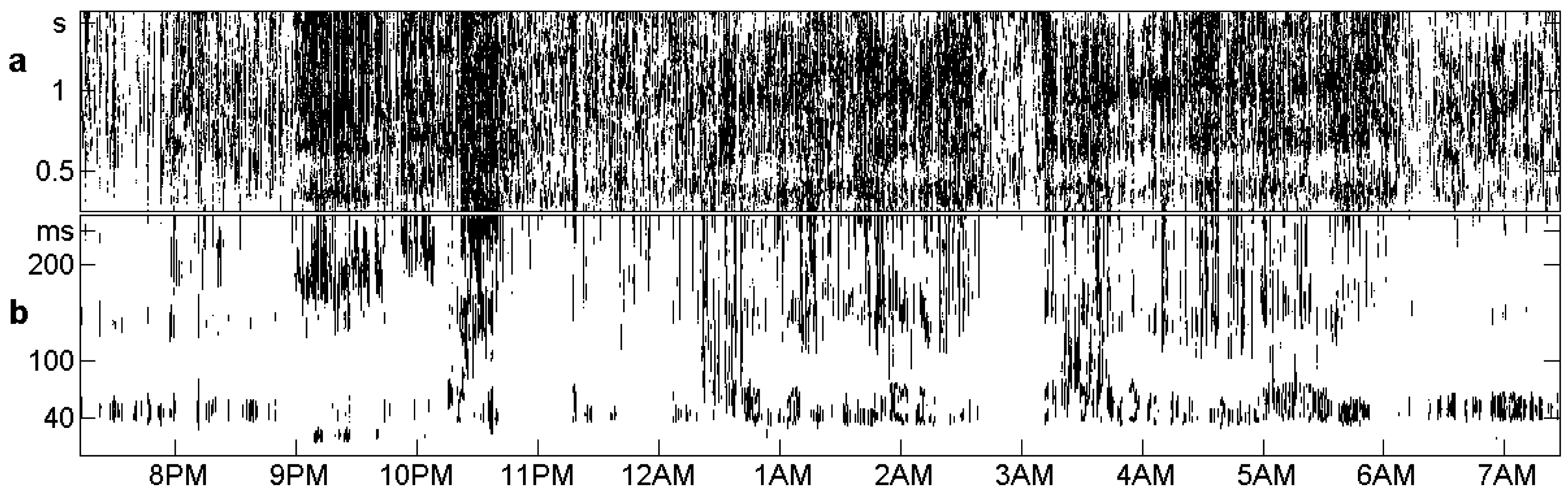
Figure 11 shows large and small values of for all windows and all d between 1 and 768, for the control n2 shown already in the top panel of Figure 5. Values smaller than are called small, and indicated by a dark dot while greater values are left white. Moreover, the d scale is divided into an upper part with s, ..., 1.5 s and a lower part ms, ..., 0.25 s, which is magnified in order to show details. The chosen threshold is three times the significance level of of Theoretically, it should correspond to a tiny p-value (cf. Section 2), but as real data are not white noise, this threshold seems appropriate [19].
In the upper part of Figure 11, the average is 0.0017, and 47% of the places have small These black spots are spread rather uniformly, so there is little chance to get information from this range of d. In the lower part, the average is 0.013, and only 10% of the places have small There is some structure related to the sleep annotations in Figure 5. There may be different choices of an interval for After some experiments, we took the bottom region, d below 40 ms, which is almost completely white. The smallest value ms was excluded since variations within 2 ms are more due to the electronic equipment than to the brain, as we knew from our own measurements. Thus, the for Figure 5, Figure 7, Figure 8, Figure 9 and Figure 10 was taken as an average over the values corresponding to ms.
Checking oscillations. Periodic phenomena have a large influence on the statistics of order patterns. As explained in [20], the persistence
assumes large negative values for and when p is the period of a periodic component. For our parameters, distance to white noise consists mainly of the persistence part, Equation (4) turns into Thus, it is natural to ask whether our was caused by certain oscillations.
In EEG measurements, a danger is contamination with mains hum, the 50 Hz frequency of the power supply. The corresponding is Since is not particularly small, there seems to be no such contamination. We should also check for alpha waves in the range 8 up to 12 Hz, although they are not likely to appear in the channel Fp2–F4. The corresponding is a d between 40 ms and 60 ms and is outside the range of our average. We conclude that our distance to white noise is not caused by oscillations.
This section should demonstrate ways to find good parameters. We do not claim that we made the best choice. Figure 6 shows that for the same person n2 an average of for d between 40 and 70 ms indicates sleep stages as large -values and REM phases by negative -values.
5. Discussion and Conclusions
Several authors used permutation entropy as a tool for EEG analysis, both in sleep medicine [7,8,9] as well as in epilepsy [12,13,14] and anaesthesia research [15]. One advantage is the robustness of ordinal parameters like and with respect to motion artefacts and low-frequency perturbations, which often appear in EEG data. While in correlation and spectral analysis, an outlier will cause an error proportional to its size, in ordinal pattern statistics, an outlier is counted as any other value.
In this note, we tried to improve the methodology by introducing distance to white noise, which can be supported by a statistical model. It was shown how good parameters can be determined. As a result, we defined an average for time spans between 4 and 40 ms, which can be considered as a measure of sleep depth on a continuous scale, very similar to the discrete sleep stages annotated by experts or by automatic scoring. A remarkable coincidence was shown in Figure 5, Figure 7, Figure 8 and Figure 9 for 20 subjects in the classical CAP sleep database of Terzano et al. [16]. A single EEG channel and short windows of 30 s gave a reliable estimate of sleep depth. Patients with insomnia had much smaller levels than healthy controls.
Although these results have to be checked with other, more recent databases, it could be confirmed that permutation entropy is a very effective tool for distinguishing sleep stages. In the present study, only length 3 patterns were used. The distance between the points, the so-called delay was varied in a wide range, so that permutation entropy and distance to white noise become functions like classical autocorrelation. Such a function is more meaningful than permutation entropy of patterns of length for delay 1.
On a general level, it was shown that the fine structure of high-resolution measurements can contain invisible information. Routine low-resolution measurement, downsampling or low-pass filtering can destroy this information, while ordinal methods have the capacity to exploit the microstructure of signals. They need to be developed further.
Acknowledgments
Costs to publish in open access were covered by Deutsche Forschungsgemeinschaft, project Ba1332/11-1.
Conflicts of Interest
The author declares no conflict of interest.
References
- Bandt, C.; Pompe, B. Permutation entropy: A natural complexity measure for time series. Phys. Rev. Lett. 2001, 88, 174102. [Google Scholar] [CrossRef] [PubMed]
- Amigo, J.; Keller, K.; Kurths, J. Recent progress in symbolic dynamics and permutation complexity: Ten years of permutation entropy. Eur. Phys. J. Spec. Top. 2013, 222, 241–247. [Google Scholar]
- Zanin, M.; Zunino, L.; Rosso, O.; Papo, D. Permutation entropy and its main biomedical and econophysics applications: A review. Entropy 2012, 14, 1553–1577. [Google Scholar] [CrossRef]
- Parlitz, U.; Berg, S.; Luther, S.; Schirdewan, A.; Kurths, J.; Wessel, N. Classifying cardiac biosignals using ordinal pattern statistics and symbolic dynamics. Comput. Biol. Med. 2012, 42, 319–327. [Google Scholar] [CrossRef] [PubMed]
- Chicote, B.; Irusta, U.; Alcaraz, R.; Rieta, J.J.; Aramendi, E.; Isasi, I.; Alonso, D.; Ibarguren, K. Application of Entropy-Based Features to Predict Defibrillation Outcome in Cardiac Arrest. Entropy 2016, 18, 313. [Google Scholar] [CrossRef]
- Amigo, J.M.; Keller, K.; Unakafova, V.A. Ordinal symbolic analysis and its application to biomedical recordings. Philos. Trans. R. Soc. Lond. A 2015, 373, 20140091. [Google Scholar] [CrossRef] [PubMed]
- Ouyang, G.; Dang, C.; Richards, D.; Li, X. Ordinal pattern based similarity analysis for EEG recordings. Clin. Neurophysiol. 2010, 121, 694–703. [Google Scholar] [CrossRef] [PubMed]
- Kuo, C.E.; Liang, S.F. Automatic stage scoring of single-channel sleep EEG based on multiscale permutation entropy. In Proceedings of the 2011 IEEE Biomedical Circuits and Systems Conference (BioCAS), San Diego, CA, USA, 10–12 November 2011; pp. 448–451. [Google Scholar]
- Nicolaou, N.; Georgiou, J. The use of permutation entropy to characterize sleep encephalograms. Clin. EEG Neurosci. 2012, 39, 202–209. [Google Scholar]
- Morabito, F.C.; Labate, D.; Foresta, F.L.; Bramanti, A.; Morabito, G.; Palamara, I. Multivariate Multi-Scale Permutation Entropy for Complexity Analysis of Alzheimer’s Disease EEG. Entropy 2012, 14, 1188–1202. [Google Scholar] [CrossRef]
- Ferlazzo, E.; Mammone, N.; Cianci, V.; Gasparini, S.; Gambardella, A.; Labate, A.; Latella, M.A.; Sofia, V.; Elia, M.; Morabito, F.C.; et al. Permutation entropy of scalp EEG: A tool to investigate epilepsies. Clin. Neurophysiol. 2014, 125, 13–20. [Google Scholar] [CrossRef] [PubMed]
- Li, X.; Ouyang, G.; Richards, A.D. Predictability analysis of absence seizures with permutation entropy. Epilepsy Res. 2007, 77, 70–74. [Google Scholar] [CrossRef] [PubMed]
- Bruzzo, A.; Gesierich, B.; Santi, M.; Tassinari, C.; Birbaumer, N.; Rubboli, G. Permutation entropy to detect vigilance changes and preictal states from scalp EEG in epileptic patients. A preliminary study. Neurol. Sci. 2008, 29, 3–9. [Google Scholar] [CrossRef] [PubMed]
- Nicolaou, N.; Georgiou, J. Detection of epileptic electroencephalogram based on permutation entropy and support vector machines. Expert Syst. Appl. 2012, 39, 202–209. [Google Scholar] [CrossRef]
- Olofsen, E.; Sleigh, J.; Dahan, A. Permutation entropy of the electroencephalogram: A measure of anaesthetic drug effect. Br. J. Anaesth. 2008, 101, 810–821. [Google Scholar] [CrossRef] [PubMed]
- Terzano, M.; Parrino, L.; Sherieri, A.; Chervin, R.; Chokroverty, S.; Guilleminault, C.; Hirshkowitz, M.; Mahowald, M.; Moldofsky, H.; Rosa, A.; et al. Atlas, rules, and recording techniques for the scoring of cyclic alternating pattern (CAP) in human sleep. Sleep Med. 2001, 2, 537–553. [Google Scholar] [CrossRef]
- Goldberger, A.; Amaral, L.; Glass, L.; Hausdorff, J.; Ivanov, P.; Mark, R.; Mietus, J.; Moody, G.; Peng, C.K.; Stanley, H. PhysioBank, PhysioToolkit, and PhysioNet: Components of a New Research Resource for Complex Physiologic Signals. Circulation 2000, 101, e215–e220. [Google Scholar] [CrossRef] [PubMed]
- Iber, C.; Anconi-Israel, S.; Chesson, A.; Quan, S. The AASM Manual for the Scoring of Sleep and Associated Events: Rules, Terminologyand Technical Specifications; American Academy of Sleep Medicine: Westchester, IL, USA, 2007. [Google Scholar]
- Bandt, C. Autocorrelation type functions for big and dirty data series. arXiv, 2014; arXiv:1411.3904. [Google Scholar]
- Bandt, C. Permutation Entropy and Order Patterns in Long Time Series. Time Ser. Anal. Forecast. 2016, 61–73. [Google Scholar] [CrossRef]
- Bandt, C. Estimation and test of permutation entropy and order patterns in time series. In preparation.
- Rényi, A. Probability Theory; Dover: New York, NY, USA, 2007. [Google Scholar]
- Rosso, O.; Martin, M.; Figliola, A.; Keller, K.; Plastino, A. EEG analysis using wavelet-based information tools. J. Neurosci. Methods 2006, 153, 163–182. [Google Scholar] [CrossRef] [PubMed]
Figure 1.
The six order patterns of length 3.

Figure 2.
(a) Example time series and (b) order pattern frequencies. The dotted line indicates
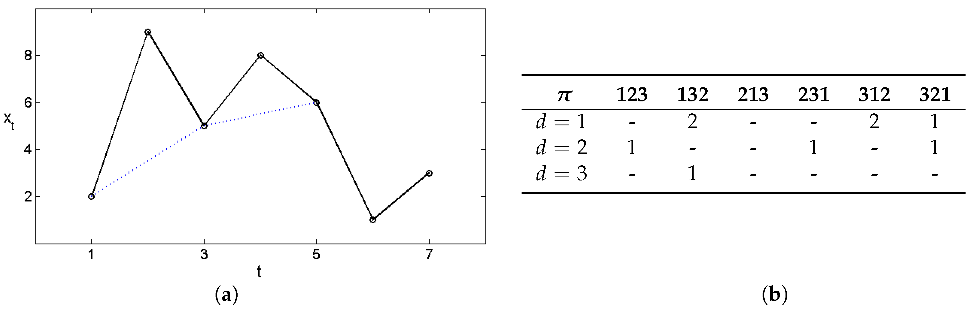
Figure 3.
Difference between H and is essentially a scale change, cf. Figure 10.
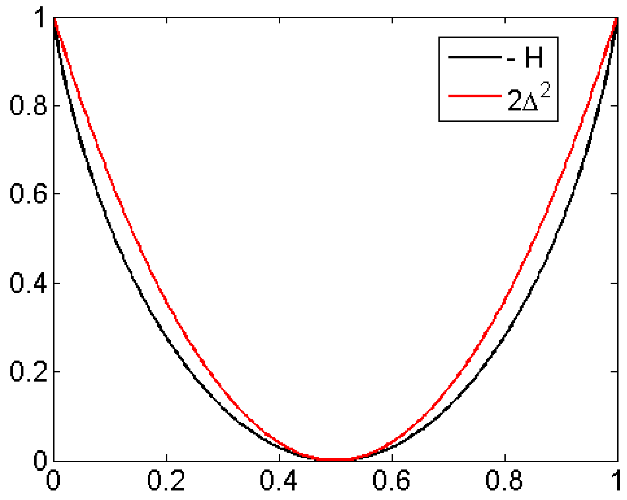
Figure 4.
Density and tail probability for standardized permutation entropy and distance to white noise, obtained from a simulation of 10 million sample series of white noise of length
Figure 4.
Density and tail probability for standardized permutation entropy and distance to white noise, obtained from a simulation of 10 million sample series of white noise of length
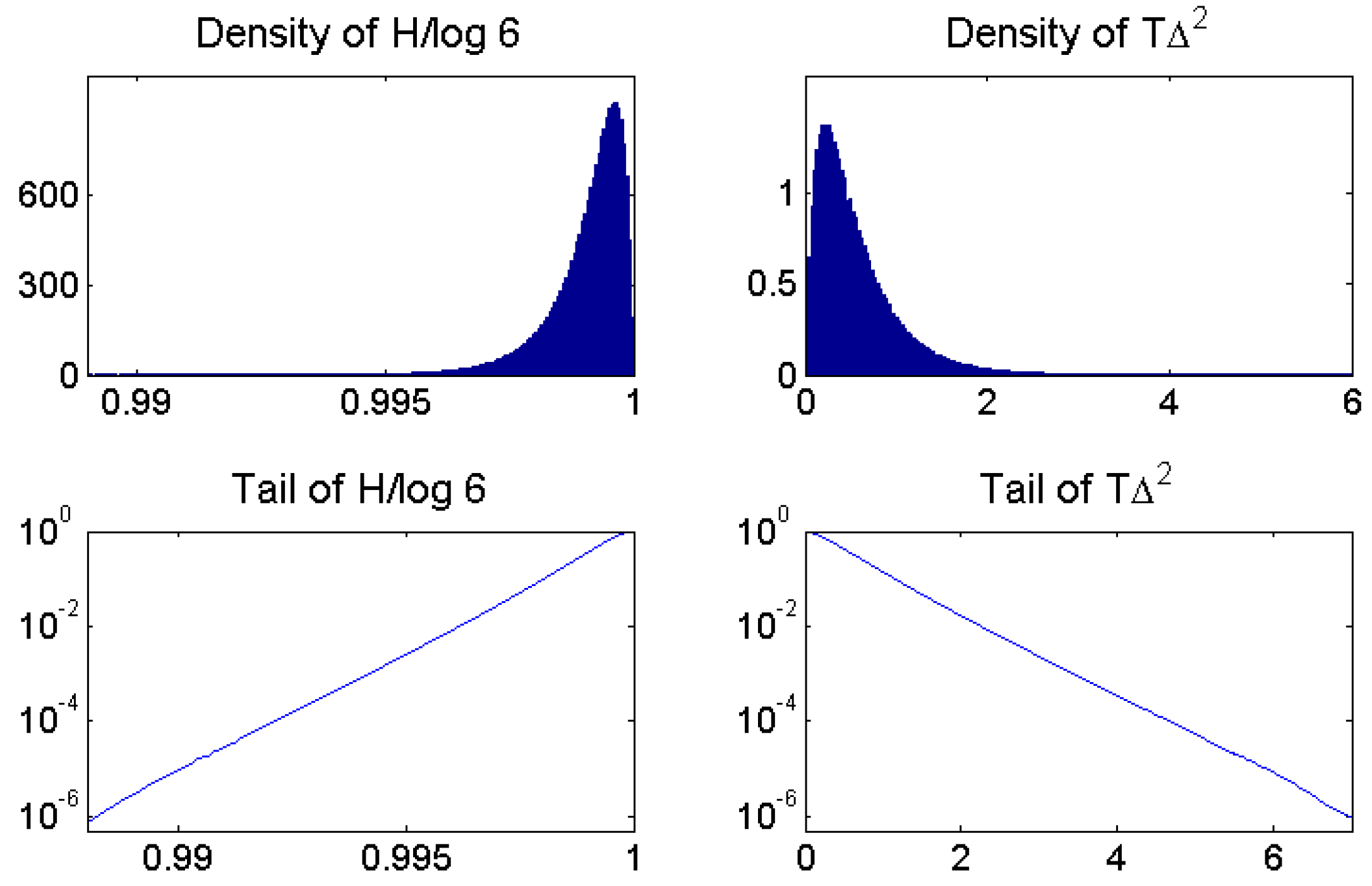
Figure 5.
Distance to white noise and expert sleep stage annotation for healthy controls in the CAP sleep database of Terzano et al. [16] available at physionet [17].

Figure 6.
An average of in Equation (5) for d between 40 and 70 ms for subject n2 indicates sleep stages and REM phases.
Figure 6.
An average of in Equation (5) for d between 40 and 70 ms for subject n2 indicates sleep stages and REM phases.

Figure 7.
Distance to white noise and expert sleep stage annotation for insomnia patients in the CAP sleep database of Terzano et al. [16].
Figure 7.
Distance to white noise and expert sleep stage annotation for insomnia patients in the CAP sleep database of Terzano et al. [16].

Figure 8.
Distance to white noise and expert sleep stage annotation for narcolepsy patients in the CAP sleep database of Terzano et al. [16].
Figure 8.
Distance to white noise and expert sleep stage annotation for narcolepsy patients in the CAP sleep database of Terzano et al. [16].

Figure 9.
Distance to white noise and expert sleep stage annotation for patients with nocturnal frontal lobe epilepsy in the CAP sleep database of Terzano et al. [16].
Figure 9.
Distance to white noise and expert sleep stage annotation for patients with nocturnal frontal lobe epilepsy in the CAP sleep database of Terzano et al. [16].
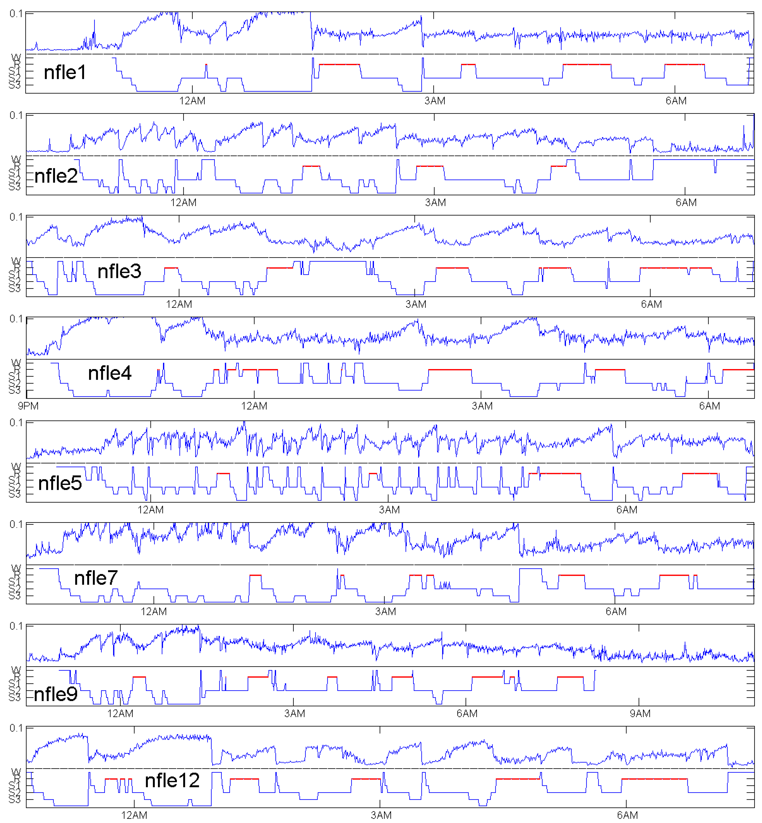
Figure 10.
Distance to white noise and permutation entropy essentially differ only by a scale change, as demonstrated here for control n11 in Figure 5. H varies between 1.4 and 1.8, between 0 and 0.1. Here, we show and , which, according to Taylor’s formula, do agree near 0.
Figure 10.
Distance to white noise and permutation entropy essentially differ only by a scale change, as demonstrated here for control n11 in Figure 5. H varies between 1.4 and 1.8, between 0 and 0.1. Here, we show and , which, according to Taylor’s formula, do agree near 0.
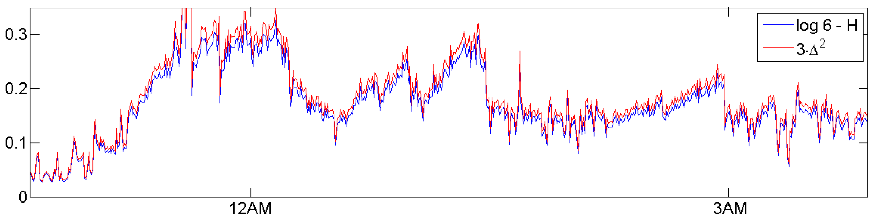
Figure 11.
Places with in the EEG record of n2 are marked black. (a) for d = 0.25, ..., 1.5 s, no structure can be seen; (b) for 0.25 s, light places are related to stages of deep sleep in Figure 5.
Figure 11.
Places with in the EEG record of n2 are marked black. (a) for d = 0.25, ..., 1.5 s, no structure can be seen; (b) for 0.25 s, light places are related to stages of deep sleep in Figure 5.

Table 1.
Critical values of (universal for ) and of (only for ) obtained from the simulation of Figure 4. Extreme values are on the left for H and on the right for
Table 1.
Critical values of (universal for ) and of (only for ) obtained from the simulation of Figure 4. Extreme values are on the left for H and on the right for
| Significance Level | 1% | 0.1% | 0.01% | 0.001% |
|---|---|---|---|---|
| 0.9962 | 0.9942 | 0.9921 | ≈0.99 | |
| 2.27 | 3.45 | 4.68 | ≈5.9 |
© 2017 by the author. Licensee MDPI, Basel, Switzerland. This article is an open access article distributed under the terms and conditions of the Creative Commons Attribution (CC BY) license (http://creativecommons.org/licenses/by/4.0/).
Share and Cite
MDPI and ACS Style
Bandt, C. A New Kind of Permutation Entropy Used to Classify Sleep Stages from Invisible EEG Microstructure. Entropy 2017, 19, 197. https://doi.org/10.3390/e19050197
AMA Style
Bandt C. A New Kind of Permutation Entropy Used to Classify Sleep Stages from Invisible EEG Microstructure. Entropy. 2017; 19(5):197. https://doi.org/10.3390/e19050197
Chicago/Turabian StyleBandt, Christoph. 2017. "A New Kind of Permutation Entropy Used to Classify Sleep Stages from Invisible EEG Microstructure" Entropy 19, no. 5: 197. https://doi.org/10.3390/e19050197
Note that from the first issue of 2016, this journal uses article numbers instead of page numbers. See further details here.