
Fractional Diffusion in a Solid with Mass Absorption


1
Institute of Mathematics and Computer Sciences, Faculty of Mathematical and Natural Sciences, Jan Długosz University in Czȩstochowa, al. Armii Krajowej 13/15, 42-200 Czȩstochowa, Poland
2
Institute of Law, Administration and Management, Faculty of Philology and History, Jan Długosz University in Czȩstochowa, Zbierskiego 2/4, 42-200 Czȩstochowa, Poland
3
Institute of Preschool and School Education, Faculty of Pedagogy, Jan Długosz University in Czȩstochowa, Waszyngtona 4/8, 42-200 Czȩstochowa, Poland
*
Author to whom correspondence should be addressed.
Entropy 2017, 19(5), 203; https://doi.org/10.3390/e19050203
Submission received: 28 March 2017
/
Revised: 24 April 2017
/
Accepted: 29 April 2017
/
Published: 2 May 2017
(This article belongs to the Special Issue Complex Systems, Non-Equilibrium Dynamics and Self-Organisation)
Abstract
:The space-time-fractional diffusion equation with the Caputo time-fractional derivative and Riesz fractional Laplacian is considered in the case of axial symmetry. Mass absorption (mass release) is described by a source term proportional to concentration. The integral transform technique is used. Different particular cases of the solution are studied. The numerical results are illustrated graphically.
1. Introduction
The conventional theory of diffusion is based on the classical Fick law, which relates the matter flux to the concentration gradient
where k is the diffusion conductivity.
In combination with the balance equation for mass, the classical Fick law leads to the standard diffusion equation
with a being the diffusivity coefficient.
Mass transport in a medium with a first order chemical reaction is described by an additional linear source term in the diffusion equation [1]:
where the values of the coefficient and correspond to mass absorption and mass release, respectively. Similarly, Equation (3) can also represent heat conduction with heat release or absorption [2]. This equation also governs heat transfer in a thin plate whose lateral surfaces exchange heat with the ambient medium having constant temperature; the values and correspond to the temperature of the medium greater and less than that of the plate, respectively [3]. Similar equations appear in the theory of bio-heat transfer [4,5,6] and in the survival probability (see [7] and references therein).
Nonclassical theories, in which the Fick law and the standard diffusion equation are replaced by more general equations, constantly attract the attention of researchers. From a mathematical point of view, the Fick law in the theory of diffusion, the Fourier law in the theory of heat conduction, and the Darcy law in the theory of fluid flow through a porous medium are identical. Some of the generalized theories are formulated in terms of diffusion, others in terms of heat conduction or fluid flow through a porous medium.
The time-nonlocal dependence between the matter flux and the concentration gradient with the long-tail power kernel (see [8,9,10,11]) can be interpreted in terms of fractional integrals and derivatives and results in the time-fractional diffusion equation
where is the Caputo fractional derivative [12,13,14]:
and is the gamma function.
The Caputo fractional derivative has the following Laplace transform rule
Here the asterisk denotes the transform, s is the Laplace transform variable.
Space nonlocal generalizations of the Fick law with the power kernel can also be interpreted in terms of fractional calculus and give the space-fractional diffusion equation
where the positive powers of the Laplace operator , , are called the Riesz derivatives.
The space-fractional heat conduction equation in the case of one spatial coordinate was considered by Gorenflo and Mainardi [15], in the case of higher dimensions by Hanyga [16]. The definitions of space-fractional differential operators can be found, for example, in [14,17,18,19,20].
The cumbersome aspects of space-fractional differential operators disappear when one computes their Fourier transforms:
where is the transform-variable vector.
It is obvious that Equation (8) is a fractional generalization of the standard formula for the Fourier transform of the Laplace operator corresponding to :
If the considered function depends only on the radial coordinate , then the two-fold Fourier transform
can be simplified (see [11,21]) and is expressed as
where . Hence, in the case of axial symmetry the two-fold Fourier transform with respect to the Cartesian coordinates x and y is reduced to the Hankel transform with respect to the radial coordinate r. Here is the Bessel function of the first kind of the zeroth order, the tilde marks the Fourier transform, the hat denotes the Hankel transform.
Equation (8) for the Fourier transform of the fractional Laplace operator in the case of axial symmetry also simplifies:
If the time nonlocality is accompanied with the spatial nonlocalty, then the general space-time-fractional heat conduction equation is obtained (see [18,19,22,23]):
It should be emphasized that fractional calculus (the theory of derivatives and integrals of non-integer order) has many important applications in description of processes in media with complex internal structure: in fractional dynamics [24,25,26,27], fractional kinetics [28,29,30], fractional thermoelasticity [8,9,31,32], biology [33,34], fractional control [35,36,37], description of physical processes in colloid, glassy and porous materials [38,39,40], comb structures [41,42], dielectrics and semiconductors [30,43,44], among others.
The fractional counterpart of Equation (3) has the following form:
Physical aspects of fractional reaction-diffusion were extensively studied in the literature (see, for example, [45,46,47,48,49] and references therein).
In this paper, we study the fundamental solutions to the Cauchy problem and to the source problem for Equation (15) in the case of axial symmetry. The integral transform technique is used. The numerical results are illustrated graphically.
2. Fundamental Solution to the Cauchy Problem
We consider the space-time-fractional diffusion equation with mass absorption (mass release) in the axisymmetric case:
under the initial condition
where is the Dirac delta function.
The constant multiplier has been introduced in Equation (17) to get the nondimensional quantities used in numerical calculations (see Equation (30)).
The Laplace transform with respect to time t and the Hankel transform with respect to the radial coordinate r give the solution in the transform domain
After inversion of the integral transforms, we get:
where is the Mittag-Leffler function in one parameter [12,14,50]:
and the following formula for the inverse Laplace transform
has been used.
The asymptotic behavior of the solution is determined by the asymptotic behavior of the Mittag-Leffler function . For , we have [51,52,53] :
Consider several particular cases of the obtained solution corresponding to different particular cases of the Mittag-Leffler function.
2.1. Standard Diffusion (, )
Since , taking into account integral (A1) from Appendix A, we get
2.2. Localized Diffusion (, )
In this case and using Equation (A2), we obtain
2.3. Subdiffusion with and
The Mittag-Leffler function can be written in the following integral form [11]:
2.4. Cauchy Diffusion with ,
For the so called Cauchy diffusion [22], which is characterized by the values , evaluating the corresponding integral (see Equation (A3) from Appendix A), we arrive at
where is the complete elliptic integral of the first kind,
Results of numerical calculations are shown in Figure 1, Figure 2, Figure 3 and Figure 4. We have introduced the following nondimensional quantities
3. Fundamental Solution to the Source Problem
In this case, we study the equation
under zero initial condition
The Laplace transform with respect to time t and the Hankel transform with respect to the radial coordinate r give the solution in the transform domain
After inversion of the integral transforms, we arrive at
where is the Mittag-Leffler function in two parameters and [12,14,50]:
and
Subdiffusion with and
The Mittag-Leffler function is presented as [11]:
Hence
4. Discussion
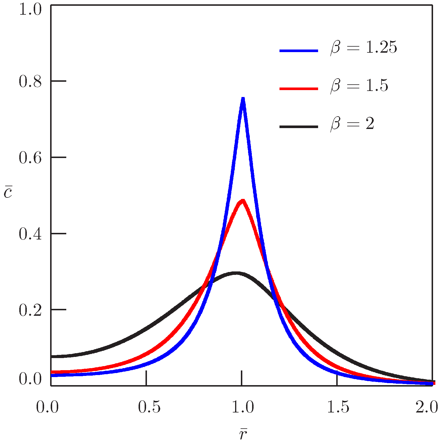
We have considered the fundamental solutions to the Cauchy problem and to the source problem for the space-time fractional diffusion equation with the linear source term. Time nonlocality deals with memory effects, whereas space nonlocality describes the long-range interaction. It is seen from Figures that for positive values of the parameter b (mass absorption) the mass concentration is decreased, for negative values of the parameter b (mass release) the mass concentration is increased. For , the shape of curves depends on the value of nondimensional time (Figure 1 presents typical results for small values of , Figure 2—for ). For fractional value of , the fundamental solution to the Cauchy problem has a cusp at . Such a cusp also appears in the curves describing the fundamental solution to the source problem for decreasing value of the order of fractional Laplacian (compare Figure 4 and Figure 6). To calculate the Mittag-Leffler functions in the fundamental solution (19) and in the fundamental solution (34) we have used the algorithms proposed in [54].
Author Contributions
Yuriy Povstenko and Tamara Kyrylych wrote the paper; Grażyna Rygał carried out numerical calculations for the fundamental solution to the source problem and prepared the corresponding Figures; Tamara Kyrylych performed numerical calculations for the Cauchy problem and prepared the corresponding Figures. All the authors have equally contributed in the discussion and overall preparation of the manuscript, as well as read and improved the final version of the manuscript.
Conflicts of Interest
The authors declare no conflict of interest.
Appendix A. Integrals
In Appendix, we present integrals used in the paper. Equations (A1) and (A2) are taken from [55], the Lipshitz-Hankel integral (A3) was evaluated in [56].
where is is the complete elliptic integral of the first kind,
References
- Crank, J. The Mathematics of Diffusion, 2nd ed.; Oxford University Press: Oxford, UK, 1975. [Google Scholar]
- Carslaw, H.S.; Jaeger, J.C. Conduction of Heat in Solids, 2nd ed.; Oxford University Press: Oxford, UK, 1959. [Google Scholar]
- Polyanin, A.D. Handbook of Linear Partial Differential Equations for Engineers and Scientists; Chapman & Hall/CRC: Boca Raton, FL, USA, 2002. [Google Scholar]
- Pennes, H.H. Analysis of tissue and arterial blood temperatures in the resting human forearm. J. Appl. Physiol. 1948, 1, 93–122. [Google Scholar] [PubMed]
- Nyborg, W.L. Solutions of the bio-heat transfer equation. Phys. Med. Biol. 1988, 33, 785–792. [Google Scholar] [CrossRef] [PubMed]
- Lakhssassi, A.; Kengne, E.; Semmaoui, H. Investigation of nonlinear temperature distribution in biological tissues by using bioheat transfer equation of Pennes’ type. Nat. Sci. 2010, 2, 131–138. [Google Scholar] [CrossRef]
- Abad, E.; Yuste, S.B.; Lindenberg, K. Survival probability of an immobile target in a sea of evanescent diffusive or subdiffusive traps: A fractional equation approach. Phys. Rev. E 2012, 86, 061120. [Google Scholar] [CrossRef] [PubMed]
- Povstenko, Y. Fractional heat conduction equation and associated thermal stresses. J. Therm. Stresses 2005, 28, 83–102. [Google Scholar] [CrossRef]
- Povstenko, Y. Theory of thermoelasticity based on the space-time-fractional heat conduction equation. Phys. Scr. 2009, 136, 014017. [Google Scholar] [CrossRef]
- Povstenko, Y. Non-axisymmetric solutions to time-fractional diffusion-wave equation in an infinite cylinder. Fract. Calc. Appl. Anal. 2011, 14, 418–435. [Google Scholar] [CrossRef]
- Povstenko, Y. Linear Fractional Diffusion-Wave Equation for Scientists and Engineers; Birkhäuser: New York, NY, USA, 2015. [Google Scholar]
- Gorenflo, R.; Mainardi, F. Fractional calculus: Integral and differential equations of fractional order. In Fractals and Fractional Calculus in Continuum Mechanics; Carpinteri, A., Mainardi, F., Eds.; Springer: Wien, Austria, 1997; pp. 223–276. [Google Scholar]
- Podlubny, I. Fractional Differential Equations; Academic Press: San Diego, CA, USA, 1999. [Google Scholar]
- Kilbas, A.A.; Srivastava, H.M.; Trujillo, J.J. Theory and Applications of Fractional Differential Equations; Elsevier: Amsterdam, The Netherlands, 2006. [Google Scholar]
- Gorenflo, R.; Mainardi, F. Random walk models for space-fractional diffusion processes. Fract. Calc. Appl. Anal. 1998, 1, 167–191. [Google Scholar]
- Hanyga, A. Multidimensional solutions of space-fractional diffusion equations. Proc. R. Soc. Lond. A 2001, 457, 2993–3005. [Google Scholar] [CrossRef]
- Samko, S.G.; Kilbas, A.A.; Marichev, O.I. Fractional Integrals and Derivatives, Theory and Applications; Gordon and Breach: Amsterdam, The Netherlands, 1993. [Google Scholar]
- Saichev, A.I.; Zaslavsky, G.M. Fractional kinetic equations: Solutions and applications. Chaos 1997, 7, 753–764. [Google Scholar] [CrossRef] [PubMed]
- Gorenflo, R.; Mainardi, F.; Moretti, D.; Pagnini, G.; Paradisi, P. Discrete random walk models for space-time fractional diffusion. Chem. Phys. 2002, 284, 521–541. [Google Scholar] [CrossRef]
- Matignion, D. Diffusive representations for fractional Laplacian: System theory framework and numerical issues. Phys. Scr. T 2009, 136, 014009. [Google Scholar] [CrossRef]
- Sneddon, I.N. The Use of Integral Transforms; McGraw-Hill: New York, NY, USA, 1972. [Google Scholar]
- Mainardi, F.; Luchko, Y.; Pagnini, G. The fundamental solution of the space-time fractional diffusion equation. Fract. Calc. Appl. Anal. 2001, 4, 153–192. [Google Scholar]
- Hanyga, A. Multidimensional solutions of space-time-fractional diffusion equations. Proc. R. Soc. Lond. A 2002, 458, 429–450. [Google Scholar] [CrossRef]
- Atanacković, T.M.; Pilipović, S.; Stanković, B.; Zorica, D. Fractional Calculus with Applications in Mechanics: Vibrations and Diffusion Processes; John Wiley & Sons: Hoboken, NJ, USA, 2014. [Google Scholar]
- Datsko, B.; Gafiychuk, V. Complex nonlinear dynamics in subdiffusive activator-inhibitor systems. Commun. Nonlinear Sci. Numer. Simul. 2012, 17, 1673–1680. [Google Scholar] [CrossRef]
- Baleanu, D.; Tenreiro Machado, J.A.; Luo, A.C.J. (Eds.) Fractional Dynamics and Control; Springer: New York, NY, USA, 2012. [Google Scholar]
- Tarasov, V.E. Fractional Dynamics: Applications of Fractional Calculus to Dynamics of Particles, Fields and Media; Higher Education Press: Bejing, China; Springer: Berlin, Germany, 2010. [Google Scholar]
- Herrmann, R. Fractional Calculus: An Introduction for Physicists, 2nd ed.; World Scientific: Singapore, 2014. [Google Scholar]
- Uchaikin, V.V. Fractional Derivatives for Physicists and Engineers; Springer: Berlin, Germany, 2013. [Google Scholar]
- Uchaikin, V.; Sibatov, R. Fractional Kinetics in Solids: Anomalous Charge Transport in Semiconductors, Dielectrics and Nanosystems; World Scientific: Hackensack, NJ, USA, 2013. [Google Scholar]
- Povstenko, Y. Thermoelasticity based on fractional heat conduction equation. In Proceedings of the 6th International Congress on Thermal Stresses, Vienna, Austria, 26–29 May 2005; Ziegler, F., Heuer, R., Adam, C., Eds.; Vienna University of Technology: Vienna, Austria, 2005; Volume 2, pp. 501–504. [Google Scholar]
- Povstenko, Y. Fractional Thermoelasticity; Springer: New York, NY, USA, 2015. [Google Scholar]
- Magin, R.L. Fractional Calculus in Bioengineering; Begell House Publishers, Inc.: Redding, CA, USA, 2006. [Google Scholar]
- Nonnenmacher, T.F.; Metzler, R. Applications of fractional calculus techniques to problems in biophysics. In Applications of Fractional Calculus in Physics; Hilfer, R., Ed.; World Scientific: Singapore, 2000; pp. 377–428. [Google Scholar]
- Caponetto, R.; Dongola, G.; Fortuna, L.; Petráš, I. Fractional Order Systems. Modeling and Control Applications; World Scientific: Hackensack, NJ, USA, 2010. [Google Scholar]
- Monje, C.A.; Chen, Y.; Vinagre, B.M.; Xue, D.; Feliu-Batlle, V. Fractional-Order Systems and Controls. Fundamentals and Applications; Springer: London, UK, 2010. [Google Scholar]
- Valério, D.; Sá da Costa, J. An Introduction to Fractional Control; The Institution of Engineering and Technology: London, UK, 2013. [Google Scholar]
- Weeks, E.R.; Weitz, D.A. Subdiffusion and the cage effect studied near the colloidal glass transition. Chem. Phys. 2002, 284, 361–377. [Google Scholar] [CrossRef]
- Hilfer, R. Experimental evidence for fractional time evolution in glass forming materials. Chem. Phys. 2002, 284, 399–408. [Google Scholar] [CrossRef]
- Kimmich, R. Strange kinetics, porous media, and NMR. Chem. Phys. 2002, 284, 253–285. [Google Scholar] [CrossRef]
- Arkhincheev, V.E. Anomalous diffusion and charge relaxation on comb model: Exact solutions. Phys. A Stat. Mech. Appl. 2000, 280, 304–314. [Google Scholar] [CrossRef]
- Arkhincheev, V.E. Diffusion on random comb structure: Effective medium approximation. Phys. A Stat. Mech. Appl. 2002, 307, 131–141. [Google Scholar] [CrossRef]
- Nigmatullin, R.R. To the theoretical explanation of the “universal response”. Phys. Status Solidi B 1984, 123, 739–745. [Google Scholar] [CrossRef]
- Nigmatullin, R.R. On the theory of relaxation with remnant temperature. Phys. Status Solidi B 1984, 124, 389–393. [Google Scholar] [CrossRef]
- Sokolov, I.M.; Schmidt, M.G.W.; Sagués, F. Reaction-subdiffusion equations. Phys. Rev. E 2006, 73, 031102. [Google Scholar] [CrossRef] [PubMed]
- Henry, B.I.; Langlands, T.A.M.; Wearne, S.L. Anomalous diffusion with linear reaction dynamics: From continuous time random walks to fractional reaction-diffusion equations. Phys. Rev. E 2006, 74, 031116. [Google Scholar] [CrossRef] [PubMed]
- Abad, E.; Yuste, S.B.; Lindenberg, K. Reaction-subdiffusion and reaction-superdiffusion equations for evanescent particles performing continuous-time random walks. Phys. Rev. E 2010, 81, 031115. [Google Scholar] [CrossRef] [PubMed]
- Méndez, V.; Fedotov, S.; Horsthemke, W. Reaction-Transport Systems: Mesoscopic Foundations, Fronts, and Spatial Instabilities; Springer: Berlin, Germany, 2010. [Google Scholar]
- Yuste, S.B.; Abad, E.; Lindenberg, K. Reactions in subdiffusive media and associated fractional equations. In Fractional Dynamics. Recent Advances; Klafter, J., Lim, S.C., Metzler, R., Eds.; World Scientific: Hackensack, NJ, USA, 2012; pp. 77–106. [Google Scholar]
- Gorenflo, R.; Kilbas, A.A.; Mainardi, F.; Rogosin, S.V. Mittag-Leffler Functions, Related Topics and Applications; Springer: Berlin, Germany, 2014. [Google Scholar]
- Erdélyi, A.; Magnus, W.; Oberhettinger, F.; Tricomi, F. Higher Transcendental Functions; McGraw-Hill: New York, NY, USA, 1955; Volume 3. [Google Scholar]
- Metzler, R.; Klafter, J. The random walk’s guide to anomalous diffusion: A fractional dynamics approach. Phys. Rep. 2000, 339, 1–77. [Google Scholar] [CrossRef]
- Metzler, R.; Jeon, J.-H. Anomalous diffusion and fractional transport equations. In Fractional Dynamics. Recent Advances; Klafter, J., Lim, S.C., Metzler, R., Eds.; World Scientific: Hackensack, NJ, USA, 2012; pp. 3–32. [Google Scholar]
- Gorenflo, R.; Loutchko, J.; Luchko, Y. Computation of the Mittag-Leffler function and its derivatives. Fract. Calc. Appl. Anal. 2002, 5, 491–518. [Google Scholar]
- Prudnikov, A.P.; Brychkov, Y.A.; Marichev, O.I. Integrals and Series, Volume 2: Special Functions; Gordon and Breach: Amsterdam, The Netherlands, 1986. [Google Scholar]
- Eason, G.; Noble, B.; Sneddon, I.N. On certain integrals of Lipschitz-Hankel type involving products of Bessel functions. Philos. Trans. R. Soc. Lond. Ser. A 1955, 247, 529–551. [Google Scholar] [CrossRef]
Figure 1.
Dependence of the fundamental solution to the Cauchy problem on distance for , , and various values of .
Figure 1.
Dependence of the fundamental solution to the Cauchy problem on distance for , , and various values of .
Figure 2.
Dependence of the fundamental solution to the Cauchy problem on distance for , , and various values of
Figure 2.
Dependence of the fundamental solution to the Cauchy problem on distance for , , and various values of
Figure 3.
Dependence of the fundamental solution to the Cauchy problem on distance for , , and various values of .
Figure 3.
Dependence of the fundamental solution to the Cauchy problem on distance for , , and various values of .

Figure 4.
Dependence of the fundamental solution to the Cauchy problem on distance for , , and various values of .
Figure 4.
Dependence of the fundamental solution to the Cauchy problem on distance for , , and various values of .
Figure 5.
Dependence of the fundamental solution to the source problem on distance for , , and various values of .
Figure 5.
Dependence of the fundamental solution to the source problem on distance for , , and various values of .
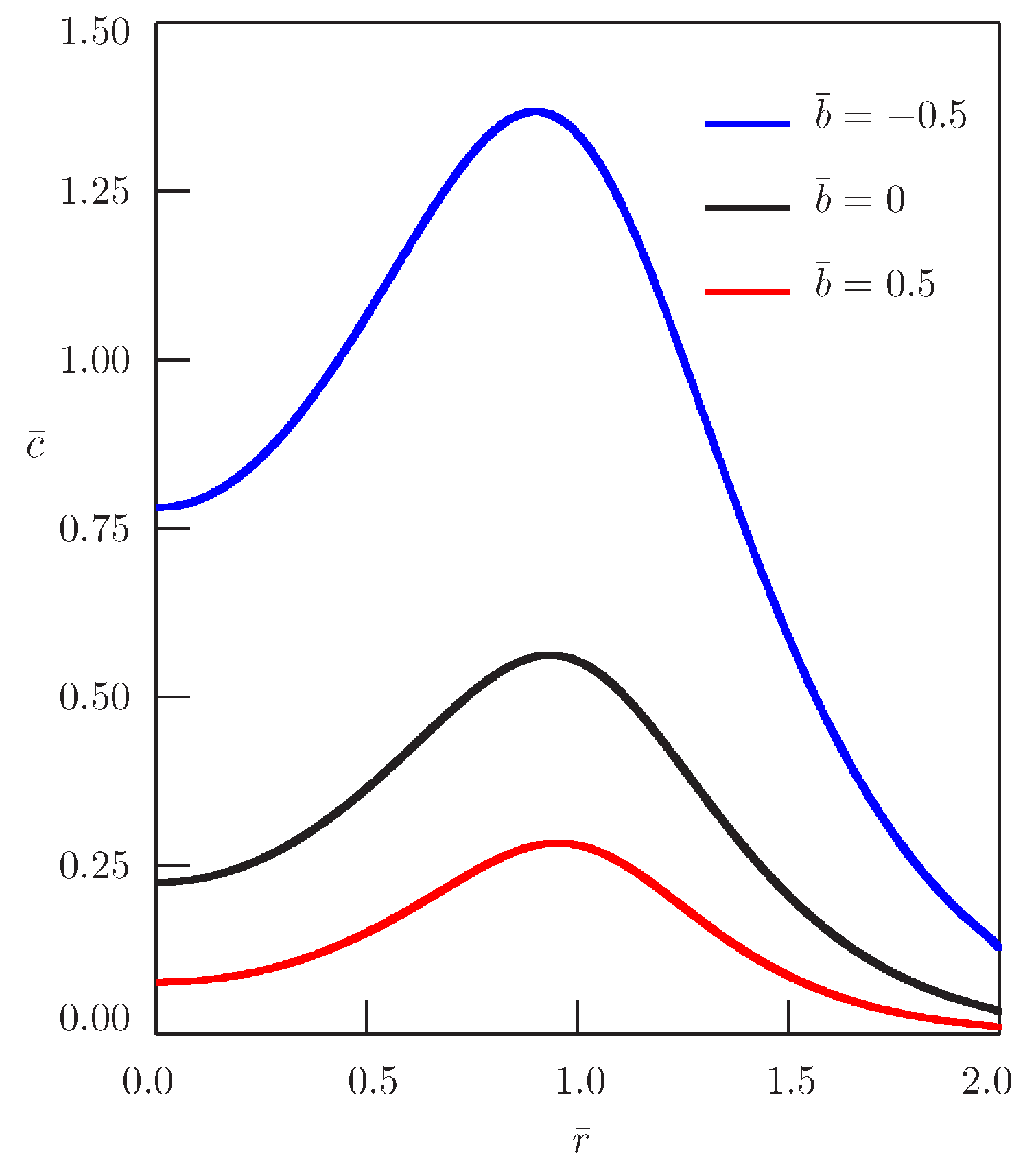
Figure 6.
Dependence of the fundamental solution to the source problem on distance for , , and various values of .
Figure 6.
Dependence of the fundamental solution to the source problem on distance for , , and various values of .
© 2017 by the authors. Licensee MDPI, Basel, Switzerland. This article is an open access article distributed under the terms and conditions of the Creative Commons Attribution (CC BY) license (http://creativecommons.org/licenses/by/4.0/).
Share and Cite
MDPI and ACS Style
Povstenko, Y.; Kyrylych, T.; Rygał, G. Fractional Diffusion in a Solid with Mass Absorption. Entropy 2017, 19, 203. https://doi.org/10.3390/e19050203
AMA Style
Povstenko Y, Kyrylych T, Rygał G. Fractional Diffusion in a Solid with Mass Absorption. Entropy. 2017; 19(5):203. https://doi.org/10.3390/e19050203
Chicago/Turabian StylePovstenko, Yuriy, Tamara Kyrylych, and Grażyna Rygał. 2017. "Fractional Diffusion in a Solid with Mass Absorption" Entropy 19, no. 5: 203. https://doi.org/10.3390/e19050203
Note that from the first issue of 2016, this journal uses article numbers instead of page numbers. See further details here.