
Measures of Qualitative Variation in the Case of Maximum Entropy

1
Department of Statistics, Yildiz Technical University, 34220 Istanbul, Turkey
2
Department of Informatics, Marmara University, 34180 Istanbul, Turkey
*
Author to whom correspondence should be addressed.
Entropy 2017, 19(5), 204; https://doi.org/10.3390/e19050204
Submission received: 13 March 2017
/
Revised: 21 April 2017
/
Accepted: 27 April 2017
/
Published: 4 May 2017
(This article belongs to the Special Issue Maximum Entropy and Its Application II)
Abstract
:Asymptotic behavior of qualitative variation statistics, including entropy measures, can be modeled well by normal distributions. In this study, we test the normality of various qualitative variation measures in general. We find that almost all indices tend to normality as the sample size increases, and they are highly correlated. However, for all of these qualitative variation statistics, maximum uncertainty is a serious factor that prevents normality. Among these, we study the properties of two qualitative variation statistics; VarNC and StDev statistics in the case of maximum uncertainty, since these two statistics show lower sampling variability and utilize all sample information. We derive probability distribution functions of these statistics and prove that they are consistent. We also discuss the relationship between VarNC and the normalized form of Tsallis (α = 2) entropy in the case of maximum uncertainty.
1. Introduction
Whenever the scale of measurement is nominal or ordinal, the classical measures of dispersion, like standard deviation and variance, cannot be used. In such cases, the only way to measure dispersion is to use measures, which involve frequencies of random observations. Wilcox [1] made the first attempt to gather some of the qualitative variation indices together pointing out the utility of these measures for statistical handling of qualitative data. One of the rare attempts of deriving probability functions for qualitative measures can be seen in Swanson [2].
Qualitative measures are widely used in social and biological sciences. Appropriate for the area of application, qualitative variation indices are preferred compared to diversity indices, or vice versa. A diversity index is a quantitative measure that accounts for the number of categories in a dataset. Measures of diversity are distinguished from measures of variation such that the former refers to counting numbers of discrete types [3]. Diversity is the antonym of concentration, whilst a near synonym of variety. The term concentration is more common in some areas of ecology, and economics. Diversity is more likely in sociology and communication [4]. For example, in economics, concentration is a measure of competitiveness in a market. The more concentrated the market, the less competitive it will be. Heip et al. [5] introduced a list of diversity and evenness indices, most of which could also be seen as qualitative variation indices. The same parallelism between qualitative variation indices and diversity indices can be found in [6,7,8,9,10] as well.
Although there are some differences in explanations of these measures, some mathematical analogies between them are straightforward for some inferential purposes. For this reason it is not surprising to find a concentration measure, which was originally proposed for measuring diversity before it was reversed (a measure is “reversed” by taking its reciprocal, or subtracting it from its maximum value, etc.). For example, Simpson’s D statistic is a measure of diversity, and “the reversed form” of it gives the Gini concentration index, which is a special case of Tsallis entropy. The Herfindahl-Hirschmann concentration index is obtained by subtracting Simpson’s D from 1.
Statistical entropy is a measure of uncertainty of an experiment as well as being a measure of qualitative variation. Once the experiment has been carried out, uncertainty is not present [11]. Thus, it can also be evaluated as the measure of information; one can get through sampling, or ignorance, before experimentation [12]. Jaynes [13] proposes that the maximizing of Shannon’s entropy provides the most appropriate interpretation for the amount of uncertainty. The principle of maximum entropy also coincides with Laplace’s well–known principle of insufficient reasoning. Pardo [14] and Esteban and Morales [15] provide theoretical background for different entropy measures.
In our study, we first present the three most common entropy measures, namely Shannon, Rényi, and Tsallis entropies with their variances, and then we discuss their asymptotic behaviour. Moreover, we list various qualitative variation indices as axiomatized by Wilcox [1], including Shannon and Tsallis entropies, and VarNC and StDev statistics. By simulations we check the normality of these measures for various entropy assumptions. We observe that maximum entropy is a serious factor, which prevents normality. We formulate the probability density functions of VarNC and StDev statistics and the first two moments under the assumption of maximum uncertainty. We also show that VarNC is special case of normalized Tsallis (α = 2) entropy under the same assumptions. We discuss the relationship between qualitative variation indices and power divergence statistics since entropy measures the divergence of a distribution from maximum uncertainty.
2. Entropy and Qualitative Variation
2.1. Common Entropy Measures
There are various entropy measures formulated by various authors in literature. Most commonly used ones are Shannon, Rényi, and Tsallis entropies. We give basic properties of these three measures below.
2.1.1. Shannon Entropy
In his study on mathematical theory for communication, Shannon [16] developed a measure of uncertainty or entropy, which was later named as “Shannon entropy”. If the discrete random variable X takes on the values
with respective probabilities
, Shannon entropy is defined as:
In case of maximum uncertainty (i.e., the case in which all probabilities are equal), this becomes
. The upper limit of Shannon entropy depends on the number of categories K. The estimator of Shannon entropy,
, is calculated by using sample information as:
where probabilities are estimated by maximum likelihood method. Although this estimator is biased, the amount of bias can be reduced by increasing the sample size [17]. Zhang Xing [18] gives the variance of Shannon’s entropy with sample size n as follows:
2.1.2. Rényi Entropy
Rényi entropy [19] is defined as:
Shannon entropy is a special case of Rényi entropy for
. The variance of Rényi entropy estimator can be approximated by:
2.1.3. Tsallis Entropy
Another generalization of Shannon entropy is mainly due to Constantino Tsallis. Tsallis entropy is also known as q-entropy and is a monotonic function of Rényi entropy. It is given by (see [20]):
2.1.4. Asymptotic Sampling Distributions of Entropy Measures
Agresti and Agresti [22] present some information about sampling properties of Gini concentration index. They also introduce some tests to compare the qualitative variation of two groups. Magurran [23] discusses some statistical tests for comparing the entropies of two samples. Agresti [24] provides the method of deriving sampling distributions for qualitative variation statistics. Pardo [14] emphasizes that entropy-based uncertainty statistics can also be derived from divergence statistics. He also discusses some inferential issues in detail. For the asymptotic behaviour of entropy measures, one may refer to Zhang Xing [18] and Evren and Ustaoğlu [25] under the condition of maximum uncertainty.
2.2. Qualitative Variation Statistics
In this section we give a list of qualitative variation indices axiomatized by Wilcox [1] and discuss sampling properties and relationship with power divergence statistic. Wilcox [1] notes that in textbook treatments of measures of variation, range, semi-interquartile range, average deviation and standard deviation are presented and discussed. However, the presentation and discussion of measures of variation suitable for a nominal scale is often completely absent. His paper represents a first attempt to gather and to generate alternative indices of qualitative variation at introductory level.
2.2.1. Axiomatizing Qualitative Variation
Wilcox points out that any measure of qualitative variation must satisfy the following:
- Variation is between zero and one;
- When all of the observations are identical, variation is zero;
- When all of the observations are different, the variation is one.
2.2.2. Selected Indices of Qualitative Variation
A list of selected qualitative variation statistics, some of which might have already been called differently by different authors in various economical, ecological, and statistical studies, are listed in Table 1.
2.2.3. Normalizing (Standardizing) an Index
In general, if an index I fails to satisfy any of the requirements in Section 2.2.1, the following transformation can be used for remedy:
Note that this has the same form as the distribution function of a uniform distribution. Since any distribution function is limited between 0 and 1, this transformation is useful in improving the situation. The term “normalization” or “standardization” is not related to normal distribution. Rather, it is intentionally used to indicate that any “normalized” index takes values from the interval
. For example, and whenever all observations come from one category, (Variation ratio)
is zero. On the other hand, when . Dividing by normalizes . In other words, normalizing this way produces the index (Index of deviations from the mode) ModVR.
2.2.4. Power-Divergence Statistic and Qualitative Variation
Loosely speaking, for discrete cases, a statistic of qualitative variation measures the divergence between the distribution under study, and the uniform discrete distribution. For the general exposition of statistical divergence measures, one may refer to Basseville [26] and Bhatia and Singh [27]. Cressie and Read [28] show that ordinary chi-square and log-likelihood ratio test statistics for goodness of fit can be taken as the special cases of power-divergence statistic. Chen et al. [29] and Harremoёs [30] explain the family of power-divergence statistics based on different parametrizations. Power-divergence statistic is an envelope for goodness of fit testing and is defined as:
where is the observed frequency, is the expected frequency under the null hypothesis, and is a constant. Under the assumption of maximum uncertainty , it becomes and:
By substituting in Equation (6), Tsallis entropy can be formulated alternatively as:
The normalized Tsallis entropy ( can also be found as:
From Equation (12), we obtain the power-divergence statistic as:
This result is in agreement with intuition. In the case of maximum entropy, normalized Tsallis entropy will be equal to one and as expected.
3. Normality Tests for the Various Measures of Qualitative Variation
3.1. Tests for Normality and Scenarios Used for the Evaluation
In order to test the normality of the above given qualitative indices under various entropy values, distributions with four, six and eight categories are studied. These distributions are chosen to investigate the differences between the behaviour of these indices in cases of both maximum entropy and lower entropy. Samples of 1000, 2000, and 5000 units are taken with corresponding runs for all distributions. The distributions are shown in Table 2, labelled from 1 to 6. Note that odd-numbered distributions correspond to maximum entropy cases. We have observed that none of the indices distribute normally for maximum entropy distributions no matter how large the sample size is. Therefore, we present only the results for lower entropy distributions.
3.2. Test Results for General Parent Distributions
To test the asymptotic normality of the indices, Schapiro-Wilk W, Anderson-Darling, Martinez-Iglewicz, Kolmogorov-Smirnov, D’Agostino Skewness, D’Agostino Kurtosis, and D’Agostino Omnibus tests are used. Success rates of these tests are shown in percentages for the non-maximum uncertainty distributions 2, 4, and 6 in Table 3. For instance, a rate 71% means five of the above mentioned seven tests accepted normality (5/7 = 0.714; the numbers are rounded to the nearest integer).
As a general tendency as the sample size increases, nine of the eleven indices tend to normality for all non-maximum entropy distributions. Nevertheless the normality of two indices, namely RanVR and the B index, is affected by dimensionality and sample size. Moreover, sampling variability of these two indices is found to be considerably higher as compared to the other nine indices. This phenomenon can be seen in the coefficient variation diagrams of indices in Figure 1 for the six distributions in Table 2 with three different sample sizes.
3.3. Test Results for Cases of Maximum Entropy
When the entropy is at the maximum, the variability of VarNC, StDev, Shannon, Hrel, and M1 statistics is comparatively low, as seen in Figure 1. On the other hand when the level of uncertainty is lower, the variability of VarNC and StDev statistics is still one among the lower scores. In addition, because of the close relationship between VarNC and StDev statistics with the chi-square distribution in case of maximum entropy, sampling properties of these two statistics can be deduced exactly; we address this issue in Section 4.
4. Sampling Properties
4.1. VarNC Statistic
The VarNC statistic is the analogous form of variance for analysing nominal distributions. It also equals the normalized form of Tsallis entropy when . The VarNC statistic can be evaluated in analogy to the variance of discrete distributions. It is defined as:
Under maximum entropy assumption, the quantity:
fits a chi-square distribution with K − 1 degrees of freedom [1]. Thus, the probability density of VarNC statistics can be written as:
If we let for and , then with we obtain:
where
It can be shown that VarNC equals the normalized version of Tsallis (α = 2) entropy with ;
VarNC is also inversely proportional to the variance of cell probabilities of a multinomial distribution. The variance of Tsallis (α = 2) entropy can be found by direct substitution of α = 2 in Equation (7):
which is larger than the variance of Tsallis (α = 2) entropy.
By deriving moments, one can show the consistency of VarNC statistics:
Under the assumption of maximum entropy, VarNC is biased since
; however, it is consistent since
, and
(see [31]). Finally, it can be noted that for larger K values,
can be approximated by a normal distribution with
and
.
4.2. StDev Statistic
The StDev statistic was proposed by Wilcox [1] as the analogous formulation of ordinary standard deviation for qualitative distributions. It is defined as:
The statistic Y = StDev is a function of
as it holds
That means that Y is
with
and
where X has the same probability density function as in Equation (16). Then by the transformation of probability densities one obtains:
where
By deriving moments, one can show the consistency of StDev statistics. By Equation (24), we write:
If we let g(x) = , by Taylor series expansion we have:
For , we get , , and .
Then we obtain:
Similarly, ignoring the quadratic and higher terms in the Taylor-series expansion yields:
StDev is biased, but consistent since, as , it holds and
4.3. Probability Distribution of VarNC and StDev under Maximum Entropy
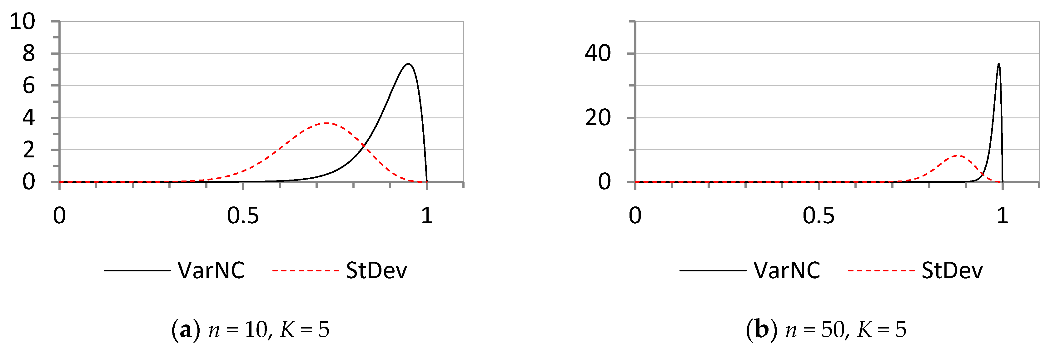
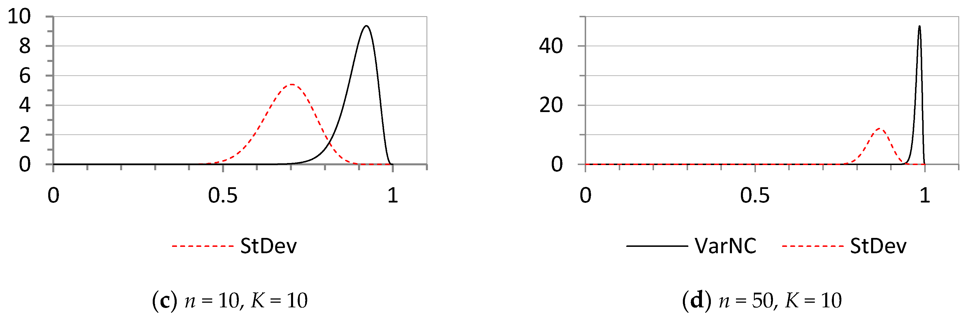
The probability distributions of the statistics VarNC and StDev under the assumption of maximum entropy are shown in Figure 2, for two different n and K values.
5. Discussion
All categorical distributions can be modelled by multinomial distribution. As the sample size increases indefinitely, multinomial distribution tends to a multivariate normal distribution. All qualitative variation statistics discussed are functions of cell counts of multinomial distribution. This fact implies the asymptotic normality of various qualitative variation measures which are simply the functions of cell counts or probabilities, themselves. In our simulation studies, we have observed this tendency for most of the investigated qualitative variation statistics whenever the uncertainty is not at maximum, except for RanVR and the B index for some dimensionalities and sample sizes. The RanVR statistic mainly uses two special numbers, the minimum and maximum frequencies. In other words, the RanVR statistic is not sufficient since it does not use all relevant sample information. For this reason, higher sampling variability is expected a priori. This situation is especially important as dimensionality (K) increases. On the other hand, the B Index is a function of the geometric mean of the probabilities. This way of multiplicative formulation of uncertainty causes higher sampling variability and may be a factor preventing normality.
None of the indices which we studied distribute normally in the case of maximum entropy, no matter how large the sample size is. This implies that maximum entropy is a factor preventing normality. Secondly, when there is little or no information about cell probabilities of multinomial distribution, the principle of insufficient reasoning justifies assuming maximum entropy distributions. In such cases, VarNC and StDev may be used in modelling the qualitative variation, since the probability distributions of these two statistics can be derived based on the relation between VarNC, StDev, and chi-square distribution. In this study we have derived the probability functions of these two statistics and shown that both statistics discussed are consistent. We have also shown that the variance of VarNC is less than that of StDev statistic and VarNC has some additional appealing properties because it is simply the normalized version of Tsallis ( when the uncertainty is at maximum.
Author Contributions
Atıf Evren and Erhan Ustaoğlu contributed to the theoretical work, simulations and the writing of this article. All authors have read and approved the final manuscript.
Conflicts of Interest
The authors declare no conflict of interest.
References
- Wilcox, A.R. Indices of Qualitative Variation; Oak Ridge National Lab.: Oak Ridge, TN, USA, 1967. [Google Scholar]
- Swanson, D.A. A sampling distribution and significance test for differences in qualitative variation. Soc. Forces. 1976, 55, 182–184. [Google Scholar] [CrossRef]
- Gregorius, H.R. Linking diversity and differentiation. Diversity 2010, 2, 370–394. [Google Scholar] [CrossRef]
- McDonald, D.G.; Dimmick, J. The Conceptualization and Measurement of Diversity. Commun. Res. 2003, 30, 60–79. [Google Scholar] [CrossRef]
- Heip, C.H.R.; Herman, P.M.J.; Soetaert, K. Indices of diversity and evenness. Oceanis 1998, 24, 61–88. [Google Scholar]
- Hill, T.C.; Walsh, K.A.; Harris, J.A.; Moffett, B.F. Using ecological diversity measures with bacterial communities. FEMS Microbiol. Ecol. 2003, 43, 1–11. [Google Scholar] [CrossRef] [PubMed]
- Jost, L. Entropy and Diversity. Oikos 2006, 113, 363–375. [Google Scholar] [CrossRef]
- Fattorini, L. Statistical analysis of ecological diversity. In Environmetrics; El-Shaarawi, A.H., Jureckova, J., Eds.; EOLSS: Paris, France, 2009; Volume 1, pp. 18–29. [Google Scholar]
- Frosini, B.V. Descriptive measures of biological diversity. In Environmetrics; El-Shaarawi, A.H., Jureckova, J., Eds.; EOLSS: Paris, France, 2009; Volume 1, pp. 29–57. [Google Scholar]
- Justus, J. A case study in concept determination: Ecological diversity. In Handbook of the Philosophy of Science: Philosophy of Ecology; Gabbay, D.M., Thagard, P., Woods, J., Eds.; Elsevier: San Diego, CA, USA, 2011; pp. 147–168. [Google Scholar]
- Rényi, A. Foundations of Probability; Dover Publications: New York, NY, USA, 2007; p. 23. [Google Scholar]
- Ben-Naim, A. Entropy Demystified; World Scientific Publishing: Singapore, 2008; pp. 196–208. [Google Scholar]
- Jaynes, E.T. Probability Theory: The Logic of Science; Cambridge University Press: Cambridge, UK, 2002; p. 350. [Google Scholar]
- Pardo, L. Statistical Inference Measures Based on Divergence Measures; CRC Press: London, UK, 2006; pp. 87–93. [Google Scholar]
- Esteban, M.D.; Morales, D. A summary on entropy statistics. Kybernetika 1995, 31, 337–346. [Google Scholar]
- Shannon, C.E. A mathematical theory of communication. Bell. Syst. Tech. J. 1948, 27, 379–423. [Google Scholar] [CrossRef]
- Paninski, L. Estimation of entropy and mutual information. Neural Comput. 2003, 15, 1191–1253. [Google Scholar] [CrossRef]
- Zhang, X. Asymptotic Normality of Entropy Estimators. Ph.D. Thesis, The University of North Carolina, Charlotte, NC, USA, 2013. [Google Scholar]
- Rényi, A. On measures of entropy and information. In Proceedings of the Fourth Berkeley Symposium on Mathematical Statistics and Probability, Los Angeles, CA, USA, 20–30 June 1961; Volume 1, pp. 547–561. [Google Scholar]
- Beck, C. Generalized information and entropy measures in physics. Contemp. Phys. 2009, 50, 495–510. [Google Scholar] [CrossRef]
- Everitt, B.S.; Skrondal, A. The Cambridge Dictionary of Statistics, 4th ed.; The Cambridge University Press: New York, NY, USA, 2010; p. 187. [Google Scholar]
- Agresti, A.; Agresti, B.F. Statistical analysis of qualitative variation. Sociol. Methodol. 1978, 9, 204–237. [Google Scholar] [CrossRef]
- Magurran, A.E. Ecological Diversity and Its Measurement; Princeton University Press: Princeton, NJ, USA, 1988; pp. 145–149. [Google Scholar]
- Agresti, A. Categorical Data Analysis, 2nd ed.; Wiley Interscience: Hoboken, NJ, USA, 2002; pp. 575–587. [Google Scholar]
- Evren, A.; Ustaoglu, E. On asymptotic normality of entropy estimators. Int. J. Appl. Sci. Technol. 2015, 5, 31–38. [Google Scholar]
- Basseville, M. Divergence measures for statistical data processing-an annotated biography. Signal Process. 2013, 93, 621–633. [Google Scholar] [CrossRef]
- Bhatia, B.K.; Singh, S. On A New Csiszar’s F-divergence measure. Cybern. Inform. Technol. 2013, 13, 43–57. [Google Scholar] [CrossRef]
- Cressie, N.; Read, T.R.C. Pearson’s χ2 and the loglikelihood ratio statistic G2: A comparative review. Int. Stat. Rev. 1989, 57, 19–43. [Google Scholar] [CrossRef]
- Chen, H.-S.; Lai, K.; Ying, Z. Goodness of fit tests and minimum power divergence estimators for Survival Data. Stat. Sin. 2004, 14, 231–248. [Google Scholar]
- Harremoës, P.; Vajda, I. On the Bahadur-efficient testing of uniformity by means of the entropy. IEEE Trans. Inform. Theory 2008, 54, 321–331. [Google Scholar]
- Mood, A.M.; Graybill, F.A.; Boes, D.C. Introduction to the Theory of Statistics, 3rd ed.; McGraw Hill International Editions: New York, NY, USA, 1974; pp. 294–296. [Google Scholar]
Figure 1.
Sampling variability of qualitative variation statistics. The vertical axis represents the coefficient of variation: (a) Distribution 1; (b) Distribution 2; (c) Distribution 3; (d) Distribution 4; (e) Distribution 5; (f) Distribution 6.
Figure 1.
Sampling variability of qualitative variation statistics. The vertical axis represents the coefficient of variation: (a) Distribution 1; (b) Distribution 2; (c) Distribution 3; (d) Distribution 4; (e) Distribution 5; (f) Distribution 6.
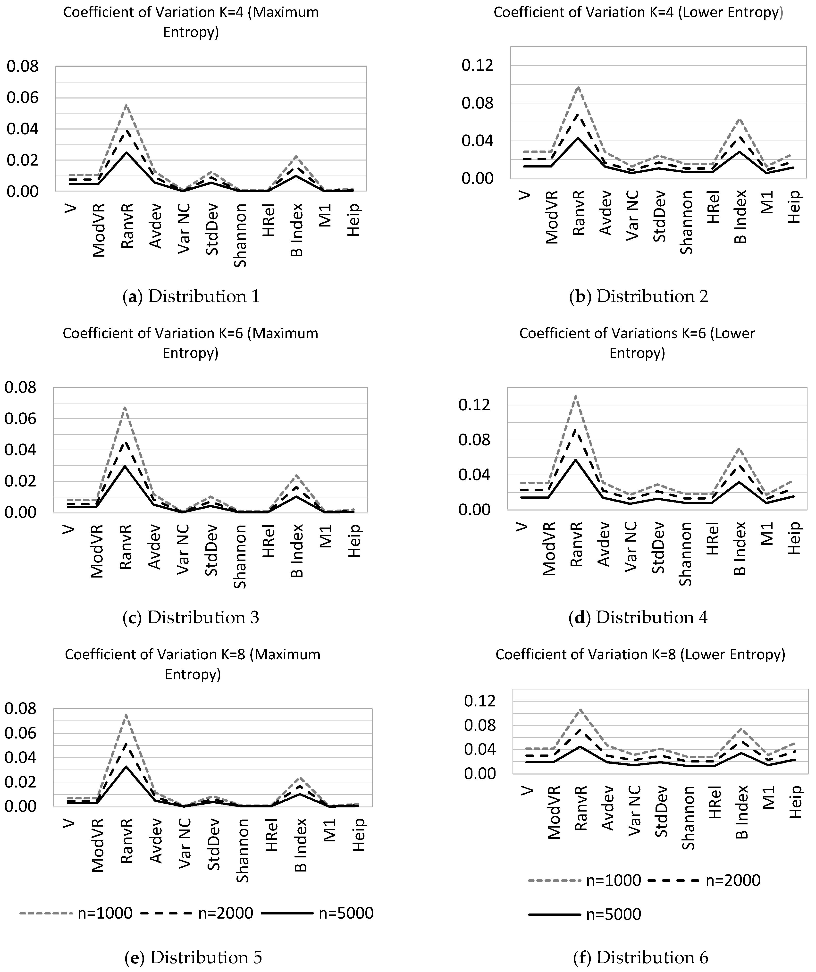
Figure 2.
The probability distributions of the statistics VarNC and StDev under the assumption of maximum uncertainty for various selected parameters n and K: (a) n = 10, K = 5; (b) n = 50, K = 5; (c) n = 10, K = 10; (d) n = 50, K = 10.
Figure 2.
The probability distributions of the statistics VarNC and StDev under the assumption of maximum uncertainty for various selected parameters n and K: (a) n = 10, K = 5; (b) n = 50, K = 5; (c) n = 10, K = 10; (d) n = 50, K = 10.


Table 1.
A list of selected qualitative variation indices ( denotes the frequency of category i, n is the sample size and K is the number of categories).
Table 1.
A list of selected qualitative variation indices ( denotes the frequency of category i, n is the sample size and K is the number of categories).
| Index | Defining Formula | Min | Max | Explanation |
|---|---|---|---|---|
| Variation ratio or Freeman’s index (VR) | 0 | is the frequency of the modal class. | ||
| Index of deviations from the mode (ModVR) | 0 | 1 | Normalized form of the variation ratio. | |
| Index based on a range of frequencies (RanVR) | 0 | 1 | are minimum and maximum frequencies. | |
| Average deviation (AVDEV) | 0 | 1 | Analogous to mean deviation. K is the number of categories. | |
| Variation index based on the variance of cell frequencies (VarNC) | 0 | 1 | Normalized form of Tsallis entropy when . Analogous to variance. | |
| Std deviation (StDev) | 0 | 1 | Analogous to standard deviation. | |
| Shannon entropy (H) | 0 | logK | The base of the logarithm is immaterial. | |
| Normalized entropy (HRel) | 0 | 1 | Normalization is used to force the index between 0 and 1. | |
| B index | 0 | 1 | B index considers the geometric mean of cell probabilities. | |
| M1 (Tsallis entropy for | 0 | It is also known as Gini Concentration Index. | ||
| Heip Index (HI) | 0 | 1 | If Shannon entropy is based on natural logarithms. |
Table 2.
Six parent discrete distributions used in the simulations.
| Distribution | 1 | 2 | 3 | 4 | 5 | 6 |
|---|---|---|---|---|---|---|
| X | f(x) | f(x) | f(x) | f(x) | f(x) | f(x) |
| 1 | 0.25 | 0.35 | 0.166 | 0.5 | 0.125 | 0.05 |
| 2 | 0.25 | 0.1 | 0.166 | 0.2 | 0.125 | 0.65 |
| 3 | 0.25 | 0.45 | 0.166 | 0.1 | 0.125 | 0.05 |
| 4 | 0.25 | 0.1 | 0.166 | 0.1 | 0.125 | 0.05 |
| 5 | - | - | 0.166 | 0.05 | 0.125 | 0.05 |
| 6 | - | - | 0.166 | 0.05 | 0.125 | 0.05 |
| 7 | - | - | - | - | 0.125 | 0.05 |
| 8 | - | - | - | - | 0.125 | 0.05 |
Table 3.
Normality results in percentages for 2nd, 4th, and 6th distributions.
| Index | Distribution 2 | Distribution 4 | Distribution 6 | ||||||
|---|---|---|---|---|---|---|---|---|---|
| n = 1000 | n = 2000 | n = 5000 | n = 1000 | n = 2000 | n = 5000 | n = 1000 | n = 2000 | n = 5000 | |
| Variation ratio | 71 | 86 | 100 | 100 | 100 | 100 | 86 | 100 | 100 |
| ModVR | 71 | 86 | 100 | 100 | 100 | 100 | 86 | 100 | 100 |
| RanVR | 100 | 71 | 100 | 100 | 71 | 100 | 100 | 86 | 43 |
| Average Deviation | 100 | 71 | 100 | 86 | 100 | 100 | 86 | 100 | 100 |
| VarNC | 57 | 100 | 100 | 14 | 100 | 100 | 100 | 100 | 100 |
| StDev | 100 | 100 | 100 | 86 | 100 | 100 | 100 | 100 | 100 |
| Shannon entropy | 71 | 100 | 100 | 14 | 100 | 100 | 100 | 100 | 100 |
| HRel | 71 | 100 | 100 | 14 | 100 | 100 | 100 | 100 | 100 |
| B index | 100 | 71 | 100 | 100 | 100 | 100 | 100 | 100 | 57 |
| M1 | 57 | 100 | 100 | 14 | 100 | 100 | 100 | 100 | 100 |
| Heip index | 28 | 100 | 100 | 57 | 100 | 100 | 100 | 100 | 100 |
© 2017 by the authors. Licensee MDPI, Basel, Switzerland. This article is an open access article distributed under the terms and conditions of the Creative Commons Attribution (CC BY) license (http://creativecommons.org/licenses/by/4.0/).
Share and Cite
MDPI and ACS Style
Evren, A.; Ustaoğlu, E. Measures of Qualitative Variation in the Case of Maximum Entropy. Entropy 2017, 19, 204. https://doi.org/10.3390/e19050204
AMA Style
Evren A, Ustaoğlu E. Measures of Qualitative Variation in the Case of Maximum Entropy. Entropy. 2017; 19(5):204. https://doi.org/10.3390/e19050204
Chicago/Turabian StyleEvren, Atif, and Erhan Ustaoğlu. 2017. "Measures of Qualitative Variation in the Case of Maximum Entropy" Entropy 19, no. 5: 204. https://doi.org/10.3390/e19050204
Note that from the first issue of 2016, this journal uses article numbers instead of page numbers. See further details here.