
About the Concept of Quantum Chaos


1
National Scientific and Technical Research Council (CONICET), Facultad de Ciencias Exactas, Instituto de Física La Plata (IFLP), Universidad Nacional de La Plata (UNLP), Calle 115 y 49, 1900 La Plata, Argentina
2
National Scientific and Technical Research Council (CONICET), University of Buenos Aires, 1420 Buenos Aires, Argentina
3
National Scientific and Technical Research Council (CONICET), University of Buenos Aires, Larralde 3440, 1430 Ciudad Autónoma de Buenos Aires, Argentina
*
Author to whom correspondence should be addressed.
Entropy 2017, 19(5), 205; https://doi.org/10.3390/e19050205
Submission received: 5 February 2017
/
Revised: 22 April 2017
/
Accepted: 23 April 2017
/
Published: 3 May 2017
(This article belongs to the Special Issue Foundations of Quantum Mechanics)
Abstract
:The research on quantum chaos finds its roots in the study of the spectrum of complex nuclei in the 1950s and the pioneering experiments in microwave billiards in the 1970s. Since then, a large number of new results was produced. Nevertheless, the work on the subject is, even at present, a superposition of several approaches expressed in different mathematical formalisms and weakly linked to each other. The purpose of this paper is to supply a unified framework for describing quantum chaos using the quantum ergodic hierarchy. Using the factorization property of this framework, we characterize the dynamical aspects of quantum chaos by obtaining the Ehrenfest time. We also outline a generalization of the quantum mixing level of the kicked rotator in the context of the impulsive differential equations.
1. Introduction
Highly unstable systems were studied in detail in many different areas of classical and quantum physics. It has been shown that a number of quantum systems have behaviors which are usually interpreted as chaotic [1,2,3,4]. However, these empirical features contrast with the fact that, in quantum systems, chaos seems to be the exception rather than the rule. Some experts even suggest that chaotic quantum systems do not exist, because the physical systems obtained from the quantization of chaotic classical systems in general do not exhibit chaotic behavior [1]. The absence of chaotic manifestations in the vast majority of quantum systems has been considered as a serious threat to the Correspondence Principle. Some radical positions have even claimed that the absence of quantum chaos challenges the empirical adequacy of quantum mechanics. Nevertheless, these positions sound surprising if we take into account the increasing attention that quantum chaos has received from the community of physicists during the last decades.
We consider that this confusing situation is the result of the conceptual disagreements about what quantum chaos is. Usually, authors define quantum chaos by analogy to the classical case, that is, by seeking indicators of chaos in the quantum domain. For instance, Peres [5] proposed an analogue to the Lyapunov exponents by means of the notion of Loschmidt echo. In turn, Loschmidt echo can be intimately related to decoherence, understood as a process occurring in open quantum systems [6]. With regard to the Lyapunov exponents, the exponential sensitivity to the initial conditions has been simulated up to a characteristic time, called Ehrenfest time or logarithmic timescale, which represents the time that a Gaussian wave packet needs to spread throughout the entire phase space [7]. The Ehrenfest timescale is a fundamental signature of quantum chaos, which characterizes the dynamical aspects of the quantum chaotic motion. Complementarily, the universal statistical properties of the energy spectrum are given by the Random Matrix Theory approach, which characterizes the stationary aspects of quantum chaos in the energy domain [8,9,10]. Another important approach to quantum chaos was proposed by Michael Berry, who identifies a chaotic quantum system as a quantum system with a chaotic classical limit [11]; he originally called the study of this kind of quantum systems chaology.
In this paper we propose a unified framework for describing quantum chaos using the quantum ergodic hierarchy, previously developed by two of us in [12,13]. We also characterize the dynamical aspects of quantum chaos by obtaining the Ehrenfest time. We will begin by considering the ergodic hierarchy of classical dynamical systems [14,15,16], which classifies asymptotic behavior in terms of the correlations between subsets in phase space. We will also consider the perspective developed by Gordon Belot and John Earman [17], who appealed to the classical ergodic hierarchy to define quantum chaos in a conceptual way that has many points in common with ours. Thus, we will extend the Belot–Earman proposal to the issue of the graininess and chaos in compatibility with the Correspondence Principle, with the purpose of develop an unified scenario for the dynamical and stationary aspects of quantum chaos. On the basis of this result, we will present a formalism developed to treat quantum systems whose classical limits belong to one of the levels of the classical ergodic hierarchy. This will allow us to identify some conditions that a quantum system must satisfy to lead to chaotic behavior in its classical limit.
In order to fulfill this task, the article is organized as follows. In Section 2, we present a brief exposition of the fundamental concepts of classical chaos. In Section 3, we introduce the classical ergodic hierarchy, its different levels and the relationships between them. Section 4 is entirely devoted to describe how the standard strategies in the literature address the problem of quantum chaos. In Section 5, we present Berry’s definition of quantum chaos, and the requirements that, according to Belot and Earman, any adequate definition of quantum chaos should satisfy. Section 6 is devoted to introduce the Weyl–Wigner–Moyal formalism as the mathematical background for our proposal. In Section 7, we describe the classical limit in terms of the mean values of the quantum observables and the weak limit. In Section 8 we review the quantum ergodic hierarchy as a framework to characterize chaotic aspects of quantum systems, based on the classical ergodic hierarchy. Moreover, we provide a generalization of the quantum mixing level of the kicked rotator, within the context of the impulsive differential equations. In Section 9, we provide a tentative unified framework for quantum chaos, based on the quantum ergodic hierarchy. For accomplish this, first we briefly review the stationary aspects of quantum chaos, by means of the quantum factorization property of quantum mixing systems. Second, we consider the dynamical features of quantum chaos and we present a deduction of the Ehrenfest time in the context of mixing systems. Finally, in Section 10 we introduce our conclusions and some perspectives for future works.
2. Classical Chaos
Chaos in classical systems is associated with high sensitivity to small variations of initial conditions [18,19]. In a chaotic classical system, small variations of the initial conditions may lead to huge differences in the future behavior of the system. In spite of the fact that classical systems are inherently deterministic, in practice chaotic properties cancel any possibility of determining their future behaviors. In other words, from an empirical viewpoint, the trajectories of chaotic systems are completely random and unpredictable.
In what follows we describe some features of classical chaos that will be necessary in order to present a unified framework of quantum chaos. We introduce two important indicators of classical chaos, the Lyapunov exponents and the Kolmogorov–Sinai entropy. Moreover, we present another approach to classical chaos based on probability density functions. All these elements will be used in Section 7 and Section 9.
- Kolmogorov–Sinai entropyWe recall the definition of the Kolmogorov–Sinai entropy (KS-entropy)within the standard framework of measure theory [14,15,16], which we will used in Section 9. Consider a dynamical system given by , where is the phase space, is a -algebra, is a normalized measure and is a semigroup of measure-preserving transformations. For instance, could be the classical Liouville transformation or the corresponding classical transformation associated to the quantum Schrödinger transformation. J is usually for continuous dynamical systems and for discrete ones. Let us divide the phase space in a partition Q of m small cells of measure . The entropy of Q is defined asNow, given two partitions and we can obtain the partition which is , i.e., is a refinement of and . In particular, from Q we can obtain the partition being the inverse of (i.e., ) and . From this, the KS-entropy of the dynamical system is defined aswhere the supreme is taken over all measurable initial partitions Q of . The positiveness of KS-entropy is a sufficient condition for the existence of chaotic motion.It should be noted that the KS-entropy is also used for characterizing the dynamical aspects of quantum chaos. Typically, in quantum systems having a chaotic classical analog, the KS-entropy and some of its quantum extensions overlap within a time range given by the Ehrenfest time. We will return to this point in Section 9.
- Lyapunov exponentsThe unpredictable behavior that characterizes chaotic systems is related to the local exponential instability of the motion [20], mathematically expressed by the Lyapunov exponents. In some cases it is enough to consider the maximum Lyapunov coefficient for characterizing the chaotic behavior. This coefficient is given bywhere is the distance, at time t, between two trajectories with initial conditions close to each other, and . It can be proved that the exponential instability of the motion implies that the highest Lyapunov exponent is positive. The prediction of the trajectory, for a sufficiently short time interval, can be characterized by the random parameter [20]:where is the precision of the trajectory’s record and is the Kolmogorov–Sinai entropy. Predictions are possible within the finite interval of “temporal determinism”, , while corresponds to the region of “asymptotic randomness”, in which almost all trajectories are unpredictable.It should be noted that, in general, the maximum Lyapunov exponent does not characterize completely the chaotic behavior of the system. There are different chaotic regimes, like chaotic, hyper–chaotic, hyper–hyper chaotic and deep chaotic, which depend on the number of positive Lyapunov exponents [21,22].
- Chaos in terms of probability density functionsLet us recall that exponential instability implies continuous spectrum [1]. In turn, this implies the decay of correlations in such a way that, for large times, the measure of the intersection between two sets of phase space, separated from each other, tends to the product of their measures. This property is called mixing, and constitutes one of the levels of the classical ergodic hierarchy. The main feature of mixing is that it establishes the statistical independence of different parts of a trajectory, when they are sufficiently separated in time. This is the main reason for the application of probability theory in the classical domain, which allows us to calculate statistical features such as diffusion, relaxation and distribution functions [1]. Consequently, this application allows us to replace the description in terms of trajectories with an equivalent one in terms of distribution functions, which, if not singular, represent not a single trajectory but a continuum of them.Due to the Liouville theorem, in classical mechanics the measure of the support of any distribution function remains constant through the entire evolution. Nevertheless, the distribution can be coarse-grained, that is, can be averaged over some domain of the phase space. The evolution of the coarse-grained distribution is described by a kinetic equation, i.e., a diffusion equation. In terms of coarse-grained distributions, the property of mixing implies that, in the asymptotic limit of infinite time, every smooth initial coarse-grained distribution converges to a constant smooth stationary state. This process is called statistical relaxation. It should be noted that this coarse-grain operation is essential to the characterization of the timescales of quantum chaos.
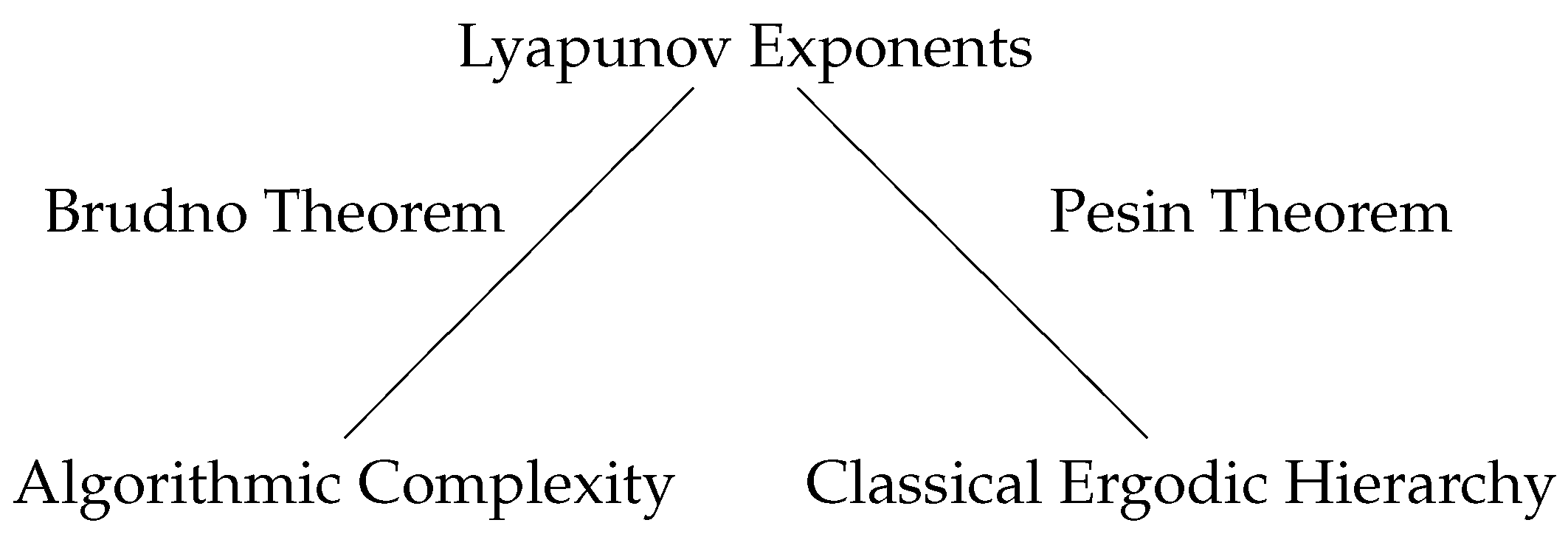
In addition to the above characterization, there are two further mathematical characterizations of chaos. One of them is the definition based on the concept of algorithmic complexity [17]; the other is formulated in the context of the classical ergodic hierarchy [14,15]. This second one classifies the different levels of instability in terms of the decay of the correlations between subsets of the phase space. Two theorems relate these three different definitions of chaos [22,23,24]: Brudno’s theorem relates algorithmic complexity to Lyapunov exponents; Pesin’s theorem relates the classical ergodic hierarchy to Lyapunov exponents. The connections among the three definitions are shown in Figure 1.
The classical ergodic hierarchy is a central element in our unified framework of quantum chaos, that we propose in Section 9, so we decided to dedicate the following section to this topic.
3. The Classical Ergodic Hierarchy
In this section, we present the ergodic hierarchy for classical systems. We define the different levels of the hierarchy and the relationships between them. The classical ergodic hierarchy will be the starting point for the development of the quantum ergodic hierarchy, introduced in Section 8.
Asymptotic behavior is one of the most important physical features of dynamical systems [4,14,15,18,19]. In this section we will present the study of dynamical systems by means of their asymptotic description in terms of correlations between subsets of phase space. The notions of ergodicity and mixing will be derived from that description. On this basis, we will introduce the classical ergodic hierarchy, which will be extended to the quantum domain in the following sections.
The classical ergodic hierarchy classifies the instability level of a dynamical system according to the type of correlations between subsets in phase space. Given a dynamical system , where is an abstract set (typically, a subset of in classical mechanics), is a –algebra of sets of , is a measure on , and is a family of measure–preserving transformations (generally, for continuous dynamical systems, , and is the classical evolution given by the Hamiltonian equations) , the following correlation between any two subsets can be defined as:
If is normalized, then can be interpreted as the probability of finding the system in A, and is simply the difference between the probability of and the product of the probabilities of A and B. Thus, in this probabilistic interpretation, measures how “independent” two subsets A and B are. This becomes clear by considering such that , from which follows that , i.e., they are independent.
The four levels of the classical ergodic hierarchy are defined in the following way. We say that the transformation , or its discrete form (where the subindex k represents the k-th time step), is:
- Ergodic, if for allor, in its discretized form, if for allWe say that a system is ergodic when the transformation is ergodic.
- Mixing, if for allor, in its discretized form, if for allWe say that a system is mixing when the transformation is mixing.
- Kolmogorov, if, for all integer r, for all , and for all , there exists a positive integer such that, if , thenwhere is the minimal algebra generated by . We say that a system is Kolmogorov (sometimes called K–system) when the transformation is Kolmogorov.
- Bernoulli, if for allfor all .
We say that a system is Bernoulli when the transformation is Bernoulli.
These levels exhibit different types of time decays according to , from the weakest level (ergodic) to the strongest (Bernoulli). The following strict inclusions hold:
Examples of ergodic and mixing transformations can be given by considering successive iterations of and respectively, over a random distribution of 1000 points in the square , where the phase space is . In Figures 4.3.3 and 4.3.4 of [15] it can be seen how in the ergodic case the distribution of points travels across the phase space retaining its shape, while in the mixing case is stretched in the direction of the straight line spreading throughout the whole phase space.
An example of Kolmogorov transformation can be given by considering the same the phase space as in the previous examples, and defining the transformation as
This transformation is known as the Baker transformation with the peculiarity that successive iterations on the rectangle mimics some aspects of the kneading dough.
With regard to the Bernoulli systems, an equivalent definition can be given using the Bernoulli shift. A Bernoulli shift is a stochastic process discretized in time, such that each independent random variable can take N distinct possible values, with the outcome i with probability , with and . The sample space is and the associated measure is the Bernoulli measure . The –algebra on X is the product –algebra given by the direct product of the –algebra of the finite set . Thus, a Bernoulli scheme is a dynamical system provided with a shift operator T, with , which is the Bernoulli shift transformation. Since the outcomes are independent, the shift preserves the measure, and thus T is a transformation which preserves the measure. Then, the alternative definition of the Bernoulli system is the following [16]: An automorphism is Bernoulli if and only if it is conjugate to a Bernoulli shift transformation.
4. What Is Quantum Chaos?
In this section we introduce the foundational approaches of quantum chaos theory along with some criticisms, which together give account for the current state–of–art of the theory.
The issue about chaos in quantum systems arose in the 70s from the attempts to understand classical chaos in terms of quantum mechanics in the classical limit. These attempts were motivated by the accumulated empirical evidence, due to Wigner [25] and Dyson [26] mainly during the 50s, coming from the study of complex nuclei and long-lived resonance states. Wigner’s central idea was that, for quantum systems with many degrees of freedom, like a heavy nucleus, one can assume that the Hamiltonian matrix elements in a typical basis can be treated as independent Gaussian random numbers. This discovery was the birth of the Random Matrix Theory (RMT), led by Mehta [9] and others [10], which made it possible to mathematically express the main prediction of the Wigner and Dyson original approach: “the statistical distribution of spacings between adjacent energy levels obeys universal distributions governed by the Gaussian ensemble of matrices.” Inspired by the universality of random matrices, in 1984 Bohigas, Gianonni and Schimt [8] formulated their celebrated statement (called “BGS conjecture”) concerning quantum chaotic systems: Spectrum of time-reversal invariant systems whose classical analogue are K-systems show the same statistical properties as predicted by Gaussian orthogonal ensembles. Furthermore, Gaussian ensembles proved to be powerful tools to study statistical properties in many applications [27,28,29,30].
At this point we consider that a classification of quantum instability in terms of stationary and dynamic properties is convenient, knowing in advance that it does not exhaust all possible approaches.
4.1. Random Matrix Theory: Stationary Aspects in the Energy Domain
As mentioned above, the origin of quantum chaos dates back to the study of atomic nuclei in the 50s, which gave rise to the RMT and to the BGS conjecture about the universality spectrum of K-systems. To further strengthen this approach, during the 80s numerical evidence began to grow: authors began to realize that the spectrum of very simple systems, like quantum chaotic billiards, also displayed the energy level fluctuations described by the Gaussian ensembles. These ensembles model the chaotic behavior of quantum systems by starting from the hypothesis of certain correlations between the matrix elements of the system’s Hamiltonian . The two conditions for the joint probability density that define a Gaussian ensemble are ([2], pp. 73–74):
where the transformed Hamiltonian is obtained from the original one by an orthogonal, unitary or symplectic transformation, depending on the corresponding type of Gaussian ensemble. Equation (12) simply represents the invariance of the density probability under an orthogonal, unitary or symplectic transformation. Equation (11) means that, in the fully chaotic regime of a chaotic quantum system, the details of the interactions are not relevant; as a consequence, the Hamiltonian can be replaced by a matrix whose elements are uncorrelated. To complete this picture, it should be noted that one of the paradigmatic models where the BGS conjecture has been more convincingly proved is the quantum billiard. This system corresponds to the stationary Schrödinger equation for a free particle of mass m that can collide with the walls of a planar domain . This problem is described by the well-known Helmholtz equation for the wave function of the particle:
subject to the Dirichlet conditions , where is the boundary of , and the eigenergies correspond to a discreet set of solutions . It can be numerically proved that, for circular domains, the system is integrable and regular, whereas for cardioid-type domains (proposed by Robnik [31]) the behavior is fully chaotic.
4.2. Heisenberg and Ehrenfest Timescales: Dynamical Aspects in the Temporal Domain
Some researches highlight a difficulty for defining quantum chaos based on classical chaos conditions [1]. They argue that some of the necessary conditions for classical chaos, like having spectrum and phase space both continuous, are violated in quantum mechanics: most quantum systems have discrete spectrum and, due to the Uncertainty Principle, the phase space is discretized by cells of finite size (for every degree of freedom). These authors consider that this problem is even more tricky when the Correspondence Principle is considered, since it states that all classical phenomena, included chaos, must emerge from the underlying quantum domain. An interesting review of this problem can be found in [32,33,34].
Some authors suggested that a possible way to reconcile the discrete spectrum of a quantum system with the Correspondence Principle is by taking into account some characteristic timescales of the quantum dynamics [1]. Others, by contrast, claim that chaos does not threaten the Correspondence Principle, but rather it expresses the emergence of the logarithmic timescale proportional to (with the dimension of the phase space). This marks out the non-commutativity of the limits and and the region where the Kolmogorov–Sinai entropy and its quantum versions agree [35,36,37,38,39]. The key point that compatibilizes both positions consists in realizing that the distinction between continuous and discrete spectrum is unambiguous only in the asymptotic limit . This idea was suggested by the implementation of numerical simulations in simple models, as the kicked rotator [1], where the dynamical aspects of quantum chaos within the proper time domain were identified. This led to a characterization of quantum chaos as a property of the time evolution that occurs within a timescale , known as Heisenberg time, after which the dynamics is governed by quantum fluctuations. Therefore, from this perspective “genuine” quantum chaos is possible only within a timescale , where the phenomena with semiclassical description, such as relaxation and exponential sensitivity, are possible. In addition, it was observed that in quantum mechanics not all chaotic phenomena occur before the Heisenberg time: there are others with a shorter lifetime. Some of this resulted in a different timescale, given by the Ehrenfest time , where is the volume of phase space explored by a classical trajectory, and is the maximum classical Lyapunov exponent that measures the exponential divergence rate between neighbouring trajectories. The Ehrenfest time can be obtained using Fourier spectra analysis based on Fast Fourier Transform or wavelets. According to [21], the latter has some advantages with regard to the other method. Even though Heisenberg and the Ehrenfest timescales characterize the limiting cases of regular and fully chaotic dynamics in quantum chaos, it should be noted that in general is necessary to consider all positive Lyapunov exponents, as was explained in Section 2.
4.3. Gutzwiller’s Trace Formula: Unifying Dynamical and Stationary Aspects
As was mentioned in Section 4.1, the universal statistical properties of quantum spectra are expected to be well described by Random Matrix Theory, without taking into account the particular details of the system under study. However, individual features such as periodic orbits or scarring phenomena are indiscernible for the RMT, since they involve the classical limit of quantum mechanics (in the limit of high quantum numbers) [2]. By establishing a correspondence between the quantum mechanical spectrum and the periodic orbits of the system, in a series of innovative works [40,41] Gutzwiller obtained the Trace Formula that describes the density of states [3]:
It expresses the quantum spectrum in terms of the properties of the periodic orbits, such as the stability matrix M, the period T, the Maslov index and the classical action . Among other things, from (14) one can derive: the Wigner semicicle law, which describes the asymptotic behavior of the eigenvalues for the average density of states, and also the Gaussian ensembles of RMT. Nevertheless, the Trace Formula presents serious difficulties when used in calculations, mainly due to the exponential number of periodic orbits that chaotic systems may have.
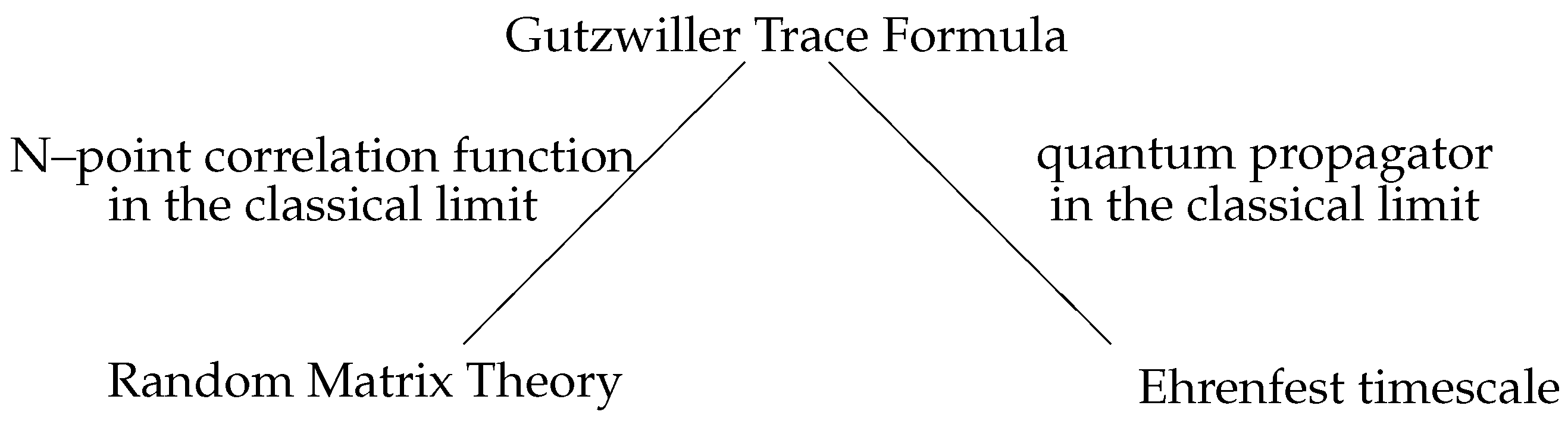
Finally, it should be said that the Trace Formula not only contains the Random Matrix Theory, but also the stationary aspects of quantum chaos, like the Ehrenfest timescale. The relationships between the Trace Formula, the Random Matrix Theory and the Ehrenfest timescale are shown in Figure 2.
4.4. Some Open Questions
At this point it is worth noting the progress toward a quantum chaos theory by means of the understanding of several features such as the RMT, the timescales, and the Trace Formula. However, at the same time many unsolved issues have emerged in the field of quantum chaos. Without the aim to be exhaustive, we conclude this section by mentioning some of the still open or partially answered questions.
- Some authors adopt a “top-down” strategy, which consists in obtaining the quantization of simple classical chaotic models by replacing classical functions with the corresponding quantum operators. In this case the conflict arises because the resulting quantum models are usually non-chaotic according to some features considered as indicators of chaos. This is the argument followed by Ford and his collaborators [42,43]: by taking the notion of complexity as the key concept to define chaos, they argue that the quantization of a classical chaotic system has null complexity and, therefore, is intrinsically non-chaotic. On the basis of this argument, the authors conclude the incompleteness of the quantum formalism: in the light of the supposed ubiquity of classical chaos, quantum mechanics should be replaced with a theory capable of accounting for chaotic behavior.
- A necessary condition for chaos in finite classical systems is the non–linearity (however, chaos may occur in linear systems, provided they are infinite dimensional [46]) of the equations of motion [47]: there must be nonlinear components coupling at least two variables together in the equation of motion. Since the quantum equations of motion are solutions of the linear Schrödinger equation, some researchers have concluded that quantum systems are necessarily non-chaotic [11]. One way out to this conclusion is the attempt to recover quantum chaos by introducing nonlinear terms in the Schrödinger equation; this could be achieved, for instance, by means of the general framework developed by Weinberg [48].
- Another feature of quantum mechanics that has been used to explain why quantum models are in general non-chaotic is the unitary character of the evolution described by the Schrödinger equation: since the time evolution of a quantum system changes neither the angle nor the distance between vectors corresponding to different states, quantum systems are not sensitive to initial conditions and, therefore, they are non-chaotic. This conclusion has led some authors to seek the way toward quantum chaos in non-unitary approaches to quantum mechanics, such as the GRW theory [49], where the collapse of the wave function is a physical process whose frequency of occurrence increases with the size of the quantum system.
- Also, a relevant approach for quantum chaos is by means of quantum thermalization [50], which is supported by cold atom experiments [51]. In this framework, it was proved that an specific initial state of an isolated and bounded quantum system of many particles tends to an equilibrium state, under the hypothesis that the energy eigenfunctions which are superposed to form that state obey the Berry’s conjecture [52,53]. The latter states that, if the quantum system has a chaotic classical limit, the energy eigenfunctions behave as if they were Gaussian random variables.
5. Quantum Chaos as Chaotic Classical Limit
In this section we discuss some strategies that consider the quantum chaos as a chaotic classical limit. We pay particular attention to the Belot–Earman program concerning to the minimal ingredients that a theory of quantum chaos should posses, along with the Zurek and Casati approaches.
Michael Berry was the first author in considering that the a precise way of characterizing quantum chaos consists in taking into account the features of the classical system that arises as the classical limit of a quantum system: A quantum system is chaotic if its classical limit is chaotic. Following Berry’s definition [11], in their paper on quantum mechanics, chaos and the Correspondence Principle, Belot and Earman [17] present a general framework for the discussion of the problem of quantum chaos. On the basis of the fact that there is no consensus about what “quantum chaos” means, they propose four requirements that any definition of quantum chaos should fulfill:
- It should possess generality and mathematical rigor.
- It should agree with common intuitions (this requirement is not considered necessary for all authors).
- It should be clearly related to criteria of classical chaos.
- It should be physically relevant.
We will take Belot–Earman’s program as the starting point of our argumentation because, among the different strategies for addressing the problem of quantum chaos, this program is the approach with more points of contact with our perspective. In the first place we consider, like Belot and Earman, that the problem of quantum chaos amounts to the problem of the emergence of classical chaos from the quantum descriptions of physical systems. In addition, we also share their view that, in turn, this is a particular aspect of the more general issue of the classical limit of quantum mechanics, that is, how classical behavior can emerge from the quantum realm.
A point of agreement with the Belot–Earman program’s is that it allows to consider the classical limit of closed systems. Whereas many authors look for quantum chaos in open systems in order to obtain non–unitary time evolutions [54,55,56,57], Belot and Earman restrict their attention to the standard quantum-mechanical treatments of closed quantum systems, by focusing exclusively on Schrödinger evolutions. However, our approach is not restricted to closed systems. We also consider that the open systems should be incorporated in a description for quantum chaos.
Another reason for adopting this perspective is the very nature of the problem: the emergence of classical chaos from quantum descriptions. Taking this into account, we have developed an approach of the classical limit of quantum mechanics [13,58,59,60,61,62] along with some of their consequences [63,64,65] according to which, under certain spectral conditions, a sufficiently macroscopic closed quantum system behaves as a classical statistical system. This approach can be related with quantum thermalization [50,51], in which the spectral condition is given by the Berry’s conjecture.
Finally, another point of agreement is related with the formalism used to address the problem. Belot and Earman point out that physicists are able to derive testable predictions from quantum mechanics with no reference to the measurement problem. This fact can be justified by a reliance on the notion of expectation values of observables and their evolutions. On this basis, the authors develop their argumentation in the language provided by the algebraic formalism of quantum mechanics. Our account of the classical limit also agrees with Belot–Earman’s approach regarding this point since, as we will see, the explanation is completely expressed in the context of the algebraic formalism and relies on the time behavior of the expectation values of the relevant observables of the quantum system.
Of course, the answer to the problem of quantum chaos strongly depends on how the classical limit of quantum mechanics is conceived. Belot and Earman introduce an index N to measure the “size” of the quantum system, in such a way that letting corresponds to taking the limit . On this basis, they focus their attention on how “mixing emerges in the limit” [17]. This means that, for the authors, the classical limit of quantum mechanics is given by the macroscopic limit. However, as we will see, there are good reasons to think that macroscopicity is not sufficient to explain the emergence of classical behavior from the quantum realm, and that decoherence is essential.
Among the strategies followed to define quantum chaos in terms of the classical limit, the following two deserve a particular interest in relation to our proposal:
- Zurek and his collaborators [55,56,57] search for chaotic behavior in open quantum systems which can undergo non-unitary time evolutions. For these authors, only the coupling between the quantum system and its environment can explain the emergence of classical chaos. In the context of their approach it can be proven that, under certain physical reasonable conditions of the environment (in particular, a Markovian environment), the von Neumann entropy of the reduced state is proportional to the Kolmogorov–Sinai entropy. Therefore, according to the Pesin theorem, the Lyapunov exponents of the classical limit can be obtained. In this way, the authors explain the emergence of non-unitary evolutions and chaos in quantum systems as a result of interaction with an environment.
- Casati and Prosen [1] consider that the emergence of classicality in closed quantum systems having a chaotic analog occurs as a result of the dephasing of the quantum interferences due to the internal dynamics of the quantum system. This characterization has been studied and numerically simulated for several chaotic billiards and for the Casati–Prosen model [66].
6. Weyl–Wigner–Moyal Formalism
In this section, we introduce some properties of the Weyl symbol and the Wigner transform that will be used to express classical quantities in terms of quantum ones, and viceversa. In Section 8, these tools will be necessary in order to obtain a quantum version of the classical ergodic hierarchy. The Weyl–Wigner–Moyal formalism maps operators on the quantum Hilbert space into distributions on the classical phase space. In terms of algebras, this transformation maps a quantum algebra of operators into a semiclassical algebra of functions. This is not the classical algebra because it is not a commutative structure, and also it contains functions that cannot be interpreted as classical distributions.
Let us consider a quantum system with degrees of freedom, represented by a Hilbert space , and an algebra of operators , defined as the ring of operators (provided with the usual sum and product), such that for all , where is the Hermitian conjugate of . For any , the Wigner transform of is the distribution function defined over given by [67]:
where . The set of all distributions is called quasiclassical algebra. In turn, the Weyl symbol of is defined as [67]:
Given two operators , the star product [68] can be introduced:
where is the metric tensor of . From the power expansion of the exponential it follows that:
where S is the value of the classical action.
The physical content of the quasiclassical algebra is given by the Moyal bracket, defined as:
From the above Eqs. it follows that the Moyal bracket is simply the Wigner transform of the quantum commutator:
Let us now consider a classical algebra , composed by all the functions and provided with the usual sum and product. The relationship between the classical algebra and the quasiclassical is given by:
where are two arbitrary functions and
is the Poisson bracket. Moreover, the Wigner transform and its inverse define the following isomorphism between and :
These applications are called Weyl–Wigner–Moyal map. When , the star product approaches the usual product (as one can see from (16)) and the Moyal bracket tends to the Poisson bracket, where is the deformation parameter. Thus, the quasiclassical algebra tends to the corresponding classical algebra. In turn, given the scalar product between two functions , a relevant property of the Wigner transformation is the following [67]:
where are any two operators of the quantum algebra.
The concepts just introduced can be applied to quantum observables and states. Observables are represented by operators belonging to an algebra , which is defined as the ring of operators such that for all , where is the Hermitian conjugate of . Quantum states are represented by the operators belonging to the positive cone of density matrices belonging to the dual space of , denoted by , that is, , with the identity operator of . The action of a state over an observable is the expectation value of in , given by , where is the trace operation. Throughout all the paper we will use the common notation for expectation values. In this case, Equation (16) expresses the expectation value of an observable in the state as the integral over of the product . In particular, for the identity function of , from (16) it follows that . As a consequence, (16) results:
which is precisely the normalization condition for the state . Since the Wigner transform of quantum states may be negative, then is not a classical algebra. For this reason, it is said that is a quasi–probability distribution, where is any density matrix of .
7. Classical Limit in Terms of Weak Limit
7.1. The Weak Limit
The classical limit of quantum mechanics refers to the study of quantum systems when the Planck constant can be neglected against other relevant magnitudes and, as a consequence, the behavior of the system can be predicted by means of the laws of classical mechanics. There are several formalisms to address the classical limit [69,70,71,72]. In this paper we will appeal to the Self-Induced-Decoherence (SID) approach, according to which observables are the fundamental items of quantum mechanics and states are functionals on them [73,74,75]. One of the main advantages of SID is that it supplies an intuitive picture of the relaxation processes of a quantum system in its approach to equilibrium in the asymptotic limit of large times, in the coarse-grained sense mentioned in Section 2.2 [1]. The SID approach is based on the notion of weak limit.
Given a quantum system represented by the algebra of observables and an initial state , if is the state at time t, then we say that is the weak limit of if
for all the observables . Equation (18) expresses the fact that can be conceived as a kind of “coarse-grained state” over the set of observables , where the expectation value approaches to the constant value for very large times. When the weak limit exists, its uniqueness follows from (18). This means that given a Hamiltonian and an initial state , there is a unique which satisfies (18) for all observable . Since the expectation value contains information about the quantum correlations of at time t, then it is reasonable to assume that represents the correlations of when , i.e., in the asymptotic limit. In this sense, can be interpreted as an “equilibrium state”.
7.2. Formulation of the Classical Limit in Terms of Weak Limit
Due to its own definition, the weak limit plays a central role in the description of the classical limit. Let S be a quantum system with a Hamiltonian . Let us denote its basis of eigenstates . Its eigenvalues constitute the quantum spectrum, i.e., the energies of the system. Depending on the quantum system, the spectrum can be discrete, continuous, complex (e.g., in non-Hermitian Hamitonians used to describe nuclear decay processes), or even a combination of them. Assuming that is Hermitian and non-degenerate, the following well-known relations hold:
Since the states are pure, for all a. Any state in the basis can be expanded as:
The state at time t is given by action of the evolution operator . More precisely:
Analogously, any observable can be expanded as:
Equation (25) captures the relevant information for our interpretation of the classical limit. It shows that the expectation value of any observable at time t has two types of terms: the diagonal terms, which are constant and their sum is denoted by , and the off–diagonal terms, which have a time dependence in function of the oscillatory factors and their sum is denoted by . In other words, expresses the quantum interference between the states of the basis , i.e., it carries the purely quantum part of . Moreover, given that the coefficients are non-negative and , then the term has the structure of a classical expectation value. By using to denote the mixed state , the term can be expressed as:
Equation (27) represents the classical limit written in terms a weak limit. On the basis of (18) and (27), the fundamental statement of the SID approach to the classical limit can be formulated [73,74,75]:
“The weak limit of a state exists if and only if the off-diagonal part can be made arbitrarily small in the asymptotic limit , which physically expresses the cancellation of quantum interference, and therefore, represents a way to establish the classical limit by means of quantum expectation values.”
For the case of quantum systems having a discrete spectrum, a way to obtain the classical limit is by requiring that the minimum spacing between two adjacent energy levels, denoted by , is much smaller than the difference between two any energy levels . Thus, the spectrum can be approximated by a continuum (as in the case of chaotic quantum billiards, such as the Sinai billiards [1,13,66]) and the sum can be replaced by a double integral:
Assuming certain conditions of regularity for the function (it is enough that ), the Riemann–Lebesgue lemma can be applied in (28) in the asymptotic limit :
When the spectrum is continuous (as in nuclear and atomic physics, and particle scattering) the condition (28) is not necessary because any quantum mean value is expressed by integrals, instead of sums. In order to use the formalism of the weak limit to characterize quantum chaos, we must first describe the behavior of a classical system in terms of its constants of motion. Given a quantum system , in the classical limit it can be represented by a classical system , with a -dimensional phase space and a Hamiltonian . According to Caratheodory’s theorem [76], has constants of motion, , which satisfy:
over maximal –dimensional hypersurfaces containing (with a short notation for ) for all point of phase space . In particular, when the union of all foliations are equal to , it is said that is integrable (this definition is equivalent to the standard one: For a Hamiltonian system having a phase space -dimensional, it is said integrable if and only if there exists a maximal set of Poisson commutative invariants, i.e., functions defined over the phase space , such that for all ). Otherwise, is non–integrable.
Now we can review the steps to recover the classical description by calculating the weak limit for states of S, as presented in [12]:
- (i)
- First, the expectation value is expressed as the sum . When the limit for is applied, the off-diagonal part tends to zero. Then, the quantum expectation value tend to the diagonal part , which has the structure of a classical expectation value.
- (ii)
- Second, the classical equilibrium density is obtained as the time-independent part of the Wigner transform of the quantum state : , where embodies the quantum effects in phase space.
- (iii)
- Finally, the classical density is expressed as a decomposition of peaked classical trajectories , (where i denotes the maximal domains ) over the hypersurfaces defined by and , with . Thus, the classical description is recovered from quantum mechanics.
The stages , , and can be summarized in the following scheme
| Quantum mechanics | Statistical classical mechanics | Classical mechanics |
| , where contains quantum correlations | , , (weak limit) | is decomposed in classical trajectories , |
These steps provide a method to address the classical limit in several phenomena like decoherence in closed and open quantum systems, statistical relaxation, and quantum chaos. The inequality warns us that in order to recover classical chaos from quantum mechanics the asymptotic limit must be taken along with the limit , according to the quantum chaos timescales. This point will be discussed in Section 9.
An example of this method was presented in [61] using a two–dimensional Sinai’s billiard, as is shown in Figure 2 [2]. The main idea is that when the particle is confined to the interior of the billiard, the trajectories can be defined by choosing two constants of motion which constitute a complete set of local constants of motion (for instance, the energy and one component of the momentum). The application of the steps – leads to an equilibrium distribution (Equation 4.25 of [61]), which corresponds to the Wigner function spread over the accessible chaotic part of phase space ([4], p. 24).
8. The Quantum Ergodic Hierarchy
This section is devoted to the quantum ergodic hierarchy developed in [12,13]. In Section 8.1 we review the construction of the quantum ergodic hierarchy and we show the consistency between the languages of measurable sets, distribution functions and quantum operators. In Section 8.2 we illustrate the ergodic, mixing and Bernoulli levels of the quantum ergodic hierarchy with the kicked rotator example, previously presented in [13]. Finally, in Section 8.3 we propose a generalization of the fully chaotic regime of kicked rotator, characterized by the quantum mixing level.
8.1. The Levels of the Quantum Ergodic Hierarchy in Terms of Quantum Expectation Values
In this subsection we review how to construct the quantum ergodic hierarchy from classical erdogic hierarchy. The resulting levels will be: quantum ergodic, quantum mixing, quantum Kolmogorov, and quantum Bernoulli. As we will see, whereas the classical ergodic hierarchy classifies classical systems according to the correlations between subsets in phase space, the quantum ergodic hierarchy classifies quantum systems in terms of correlations between states and observables. For accomplish this, we will need the tools described in Section 6, such as of the Wigner transformation and the Weyl symbols.
Let us begin with the important remark that the correlation function relevant to the ergodic hierarchy, , can be equivalently expressed in several mathematical formalisms. This is a key point in order to pass from the classical ergodic hierarchy to its quantum version. We will employ the following three languages to express the correlation .
- (a)
- The language of measurable sets:
- (b)
- The language of distribution functions:where is the identity function on .
- (c)
- The quantum language:where are two any operators.
In order to show the relationships between (a), (b) and (c), we will restrict to the families of measurable sets and functions, which are big enough for all practical purposes (for the case of non–measurable functions and sets this analysis should be made more carefully).
- (a) and (b): By definition, ; then, from (29) the correlation function reads:Let be two distribution functions defined over . They can be expanded in terms of characteristic functions as:where are countable partitions of . Now, using (32) for each and , multiplying both members by and finally adding over the indexes , we obtain:Then, from (33), the following relation can be obtained:where the correlation of (b) has been recovered.
- (b) and (c): Let be two observables, and consider the functions and . In particular, from (30) the correlation function can be written as:
Therefore, the languages (a), (b), and (c) are equivalent and can be exchanged.
In order to describe the evolution of any initial distribution function, we must consider a classical evolution operator that plays a role analogue to that of the quantum one. Given the dynamical system and a distribution function f defined on , the Frobenius–Perron operator associated to the transformation acts over f as [15]:
Just as the weak-limit states are fixed points of the quantum evolution operator in the sense of the expectation values, the distribution functions are fixed points of the Perron operator. As might be expected, the are physically interpreted as equilibrium distributions, since they are invariant under the evolution, i.e., . In a generic case, there may be several fixed points . However, in the case of an ergodic dynamical system, there is only one ([15], p. 45). Moreover, it can be shown that is a fixed point of if and only if:
is an invariant measure under the transformations ([15], p. 46).
It is interesting to note that admits an intuitive interpretation from the viewpoint of statistical mechanics. If is interpreted as the density of points in phase space of the system in the asymptotic limit, then it is nothing but the density distribution of the Liouville equation, whose evolution is given by the Liouville theorem [4,18,19,22]:
where is interpreted as a situation of statistical equilibrium where the volumes in phase space do not change through time. This motivates the definition of a new correlation function in terms of :
Given a state at time t and an observable , the task is to obtain the quantum correlation between and . Using (38) and the properties of the Wigner transform, the correlation relevant to the quantum ergodic hierarchy turns out to be [12,13]:
where is the representative state of equilibrium in the sense of the expectation values, such that . Then, by replacing with in each level of the classical ergodic hierarchy (Equations (4)–(9)), the levels of the quantum ergodic hierarchy are obtained. Precisely, if is the state at time t, the quantum evolution operator is
- Quantum ergodic ifor, equivalently in its discretized form, ifwhere is the initial state after k time steps and the operator is any unitary operator representing the time evolution. In general, , where is the Hamiltonian of the quantum system and is any sequence of discretized time steps.
- Quantum mixing ifor, equivalently in its discretized form, if
- Quantum Kolmogorov if, for all the set of observables and for all the ,
- Quantum Bernoulli if
The state is precisely the weak limit for the quantum mixing, the quantum Kolmogorov and the quantum Bernoulli levels. It can be shown that, for the quantum ergodic level, is the Cesaro weak limit [12]. Moreover, the condition of non-integrability of the Hamiltonian of the quantum system under study must be added; otherwise, the unidimensional quantum harmonic oscillator would be ergodic, which makes no sense since its classical limit is the classical harmonic oscillator that is non-ergodic. Before introducing an example of this theoretical proposal, we will conclude this subsection with some remarks:
- (i)
- The correlation between subsets in phase space of the classical ergodic hierarchy is translated into a correlation between states and observables in the quantum ergodic hierarchy. Analogously to the classical case, it is an asymptotic characterization of the quantum systems.
- (ii)
- Quantum mixing implies weak limit but the conversely it is not true. For instance, the quantum harmonic oscillator has weak limit for high quantum numbers, but its classical limit is not mixing.
- (iii)
- The quantum Kolmogorov level implies a condition over the set of observables on which it is defined, due to the presence of a –algebra in its classical definition.
- (iv)
- As in the classical ergodic hierarchy, the following strict inclusions hold:
8.2. The Kicked Rotator: A Paradigmatic Example of Quantum Chaos
Once the ergodic quantum hierarchy has been defined as an alternative characterization of quantum chaos, it is desirable to test its relevance with an example that manifests several indicators of chaotic behavior in the quantum domain. For this purpose, we will review a paradigmatic example in the field: the kicked rotator, presented in [13].
The kicked rotator is one of the most studied systems in the literature about chaos [1,2,3]. It expresses in a simple way the physics of classical chaos when described in terms of a classical Hamiltonian of the type , where is the unperturbed part and represents a perturbation depending on a continuous parameter that typically breaks the integrability of . Classically, different regimes of the dynamics can be distinguished as varies, from the regular and integrable regime for to a critical value , characteristic of the system, where a chaotic sea surrounding islands of stability emerges in phase space. For almost all phase space is covered by the chaotic sea, with only a few stability islands; this corresponds to the regime known as fully chaotic.
The relevance of the kicked rotator lies in the fact that the dynamics of several chaotic classical quantum systems can be mapped onto its dynamics. The quantum Hamiltonian of the kicked rotator is ([2], p. 145):
which describes the free rotation, in an angle , of a pendulum, whose angular moment is being kicked at intervals of period by a gravitational potential of strength , where the moment of inertia has been normalized. An adequate description of the dynamics is given by the Floquet operator as the evolution operator, which, according to the periodicity of the potential, is given by:
It should be noted that the Floquet operator is the quantum version to the classical one, used for describing the stability of orbits in classical Floquet theory. More precisely, consider an impulsive differential equation and for some . Then, the study of the stability properties of a periodic orbit with period () can be done by considering a stroboscopic classical map, which takes the form
It is interesting to note that provides an analog stroboscopic description of (48) about the quantum system. In the quantum case, the time evolution is discretized by the finite and equally time steps . Given the eigenfunctions basis of the Floquet operator , whose eigenvalues are the well-known Floquet phases ([2], p. 137). As well as the eigenvalues of the classical map (48) determine the stability of the periodic orbits, the Floquet phases characterize the type of dynamics in the quantum case, as we shall see for the fully chaotic regime of the kicked rotator.
Any initial state can be expressed in that basis as:
In order to obtain after N time steps, corresponding to the time , one must apply N times the operator on , obtaining:
where the first and the second sums of (50) contain the diagonal and the off-diagonal terms of respectively.
Now we are able to characterize the dynamical regimes of the kicked rotator by means of the levels of the quantum ergodic hierarchy introduced above. We begin by recalling that the case corresponds to a pseudointegrable and regular behavior. In this regime the dynamics is almost equal to the free pendulum and, therefore, integrable: the system is not unstable.
8.2.1. Diffusive and Stochastic Regime in Terms of the Quantum Ergodic Level
When the system enters into the non-integrable regime and its behavior becomes stochastic and diffusive. In this regime, in the regular zones of the phase space, the stability islands coexist with the chaotic sea. If one chooses initial conditions in the chaotic sea, the rotor will eventually explore all the accessible phase space. Non-integrability allows us to apply the analysis by using the quantum ergodic level.
Since the time evolution is discretized, then it is convenient to use the definition given by (41). Let be an observable, then, by applying (50), the expectation value of in at time is:
with . The double sum in corresponds to the quantum interference terms, while the first sum is its “classical” part that can be interpreted as a classical statistical expectation value. From (51) and , it follows that:
where, since the spectrum is not degenerate, we have used that:
Therefore, Equation (52) expresses the fact that the kicked rotator is quantum ergodic for . In this case, is the Cesaro limit of , since represents a “time-averaged” equilibrium state: tends to in a temporal average.
8.2.2. Fully Chaotic Regime and Exponential Localization in Terms of the Quantum Mixing and the Quantum Bernoulli Levels
When , the behavior becomes completely chaotic: the characteristic phenomenon of this regime is the exponential localization. Indeed, in this case the expected quantum distribution for the quadratic expectation value of the angular moment after N kicks is given by ([2], p. 149):
where is the localization width. Exponential localization implies that, for a number of kicks , the system remains in the classical diffusion regime. Whereas for the system is in the fully chaotic regime and the phases in oscillate so fast that only the diagonal terms in (51) survive. This is the phenomenon known as dephasing, which constitutes one of the peculiarities of quantum chaos [1]: the state decoheres to its weak limit , and the quantum expectation values acquire a classical structure, that is, . This means that:
with . According to the discretized version of the quantum mixing level, Equation (53) shows that the kicked rotator is quantum mixing for .
The decoherence time for the dephasing process can also be estimated. Since for the phases in oscillate very fast, then from the off-diagonal part of the expectation values tend to cancel. Therefore, the decoherence time can be approximated as , so it turns out to be a function of the time step and the localization width . Since for the expectation values read , then according to the quantum ergodic hierarchy, the kicked rotator enters into the quantum Bernoulli level when .
We can summarize the behavior of the kicked rotator in terms of the quantum ergodic hierarchy in the following scheme:
| QEH does not apply | Quantum ergodic | Quantum mixing |
| - | - | Quantum Bernoulli for |
| Integrable and | Non-integrable, | Non-integrable, |
| regular | diffusive–stochastic | fully chaotic |
8.3. Generalizing the Kicked Rotator
In this section, we propose a generalization of the fully chaotic regime of kicked rotator, characterized by the quantum mixing level, within the context of impulsive differential equations.
The classical kicked rotator is described by the following differential equations
where again the moment of inertia has been normalized. These equations corresponds to a particular case of impulsive differential equations of the type
where and . In what follows we propose a generalization of the kicked rotator description. It is based on two facts: (i) the analogy between the eigenvalues of the stroboscopic map (48) and the Floquet phases, and (ii) the randomness of the Floquet phases.
Consider a quantum system having a Hamiltonian . Assume that its classical analogue has a classical Hamiltonian given by an impulsive differential equation as (55), with
9. Towards a Unified Theory of Quantum Chaos
In physics, the degree of success ascribed to a theory is mainly given by its ability to predict old and new phenomena, in the context of an independent framework as synthetic as possible in terms of its principles and expressed in the simplest possible way. The synthesis of electrical and magnetic phenomena given by Maxwell’s electromagnetic theory and Einstein’s theory of relativity are examples of this stance. However, this does not seem to be the case of quantum mechanics, since its formulation usually requires an observer or an object that obeys classical mechanics, with which the quantum system under study interacts. Moreover, the Correspondence Principle implies that all classical phenomena must be recovered from quantum mechanics in the classical limit. Therefore, if the description of quantum chaos is in the scope of quantum mechanics—as presumably one would wish—it can be expected that such description inherits the dependence with respect to classical mechanics. In fact, the approaches to quantum chaos that remain independent of classical mechanics, such as the Random Matrix Theory, have limitations to explain fine details of the quantum chaotic spectrum, as scarring phenomena or periodic orbits. Moreover, although Gutzwiller’s Trace Formula unifies the stationary and the dynamical aspects of quantum chaos, the price to pay is too high due to the exponential amount of information needed to use it. Given these peculiarities, the search of a theory of quantum chaos that unifies all its aspects still seems an incomplete task.
In this section we propose a tentative unified framework for quantum chaos, based on the quantum ergodic hierarchy. To accomplish this task, in Section 9.1, we briefly review the stationary aspects of quantum chaos [65], by means of the quantum factorization property of quantum mixing systems. Then, in Section 9.2, we consider the dynamical features of quantum chaos. In particular, we present a deduction of the Ehrenfest time in the context of mixing systems.
9.1. Stationary Aspects from Quantum Factorization Property
In this subsection we resume the stationary aspects of quantum chaos based on a quantum version of the factorization property of mixing systems, called quantum factorization property. This results were previously developed in [65]. For the sake of brevity the lemmas and theorems presented below do not contain their proofs since they can be found in the corresponding references included in the text.
As we have seen in Section 4, the manifestation of chaotic features in quantum systems is possible within the characteristic timescales, where the semiclassical and quantum descriptions overlap and the statistical predictions of the Gaussian ensembles are displayed [1,2,3,11]. Thus, within the logarithmic timescale, it may be expected that the states have statistical properties, as the randomness and the invariance conditions given by Equations (11) and (12), but now expressed in terms of quantum correlations. In addition, for quantum systems belonging to the quantum mixing level, the quantum correlations are expressed by means of the weak limit. Therefore, there should be some kind of connection between the statistical properties of quantum chaos and the correlations of the quantum mixing level.
From the level of quantum mixing, Gaussian ensembles can be obtained by means of a condition that mixing correlations satisfy, i.e., the factorization property [65]. For the mixing level of the classical ergodic hierarchy, the following result can be obtained:
Lemma 1 (Factorization property).
Let be a normalized distribution which is a fixed point of the Frobenius-Perron operator . If are the n characteristic functions of n subsets , then
In the limit , using this Lemma (where is the dimension of the phase space), the following quantum version can be obtained:
Theorem 1 (Quantum factorization property).
Let us consider a quantum system belonging to the quantum mixing level. Then, for a set of observables , when the following relation holds:
Both Lemma 1 and Theorem 2 express a distinctive property of mixing systems in the asymptotic limit: the randomness of the correlations between invariant densities (or weak limits in the quantum case) and a product of characteristic functions (or a product of observables in the classical limit, for the quantum case).
Now, by Born rule, the trace of a projector acting over a state is interpreted as the probability that the fact represented by occurs when the system is in state . This gives us a clue to express probabilities as traces of projectors. In particular, if N is the dimension of the quantum Hamiltonian, it can be shown that the differential probabilities and are:
where , , and are a weak limit and certain projectors depending on the variables and the differentials . Moreover,
This construction, along with the quantum factorization property of Theorem 2, allows us to obtain the Gaussian ensembles in the classical limit in a simple way:
Theorem 2 (Gaussian ensembles distributions from the quantum mixing level).
Let us assume that S is a mixing quantum system, and the are the matrix elements of its Hamiltonian .
- (i)
- In the classical limit the randomness condition can be obtained:
- (ii)
- Let us consider the transformed variables corresponding to through the change of variables , where stands for the transpose, complex transpose, or dual of if is orthogonal, unitary, or symplectic, respectively. Let be the transformed probability density function of . In the classical limit the invariance condition can be obtained:
the formalism of the quantum ergodic hierarchy, as a particular case of the quantum mixing correlations in the classical limit.
9.2. Dynamical Aspects from KS-entropy and Factorization Property
In this section, we consider the dynamical features of quantum chaos and we obtain the Ehrenfest time in the context of mixing systems. In order to do that, we apply the factorization property of Section 9.1 and the graininess of quantum phase space to obtain an estimation for the Kolmogorov–Sinai entropy.
We begin by employing the mixing correlations described in Section 9.1. We consider a quantum system having N degrees of freedom. Thus, the discretized quantum phase results –dimensional and composed by rigid cells of minimal size , where ℏ the Planck constant and stands for . We assume that the dynamics is mixing and therefore, chaotic. This implies that the dimension must be , since closed systems with are all integrable. In particular, we consider the system occupies a bounded compact region with and (otherwise is normalized). This assumption fits adequately with the chaotic billiards and with some non integrable systems under a central potential (for instance, the Henon–Heiles system).
By the Uncertainty Principle it follows that there exists a maximal partition (that is, the greatest refinement that one can take) of composed by M identical and rigid rectangle cells of dimensions and for all where M is the maximal number of cells that intersect . Since and is a partition we have that , that is
Equation (57) expresses the graininess of the quantum phase space. In order to obtain the KS-entropy now the key point is to consider the timescale in which the classical and quantum descriptions overlap. Let be this timescale. Since one can recast (2) as
Finally, from this equation one can express as
The main role of the time rescaled KS-entropy is that allows to introduce the timescale as a parameter.
Therefore, the supreme in (58) can be replaced by in the context of the graininess of the quantum phase space. Now, the partition is given by
Given a –uple and since the dynamics is bounded and contained in the compact then one has that for all . Thus, one can express as
Since it is clear that is a normalized distribution. Moreover, is a fixed point of the Frobenius–Perron operator associated with the transformation due to the measure is trivially which by definition is invariant under . Then, given the distribution and the characteristic functions one can apply the Lemma 1, thus obtaining
That is,
and since for all the Equation (61) implies
Also, since the preserves then one has
and given that all the elements of have the same volume then from (64) one obtains
To complete the calculus one needs to know the number of –uples . The most simplified situation is to consider that the mixing dynamics is such that for all n and the sets are all different. In other words, one has M possibilities for , the same for and so on. This means that
which expresses that is an upper bound for the number of that give rise to different subsets . From the graininess condition (57) and Equations (66) and (67) one has
This equation states that the entropy of can grow, at most, as a linear function of the time. Finally, replacing the supreme in (58) by the limit one obtains
Now, since then we arrive to our main result of the paper:
which is the upper bound sought for the KS-entropy in terms of the Planck constant ℏ and the timescale . When is not normalized the graininess relation reads as . Then, in the general case one can replace by with the quasiclassical parameter. Doing this, the timescale can be expresses as
which is nothing but the Ehrenfest time [1]. One final remark that deserves to be mentioned is the following. From (70) one can see that the upper bound diverges in the classical limit . This is interpreted by some authors [35,36,37,38,39] as a manifestation of the non commutativity where the first order leads to classical chaos and the second one represents a quantum behavior with no chaos at all.
10. Conclusions
The main objective of this work was the search for a unified framework satisfying the main signatures of quantum chaos. This task requires two conditions, at least. On the one hand, the imitation of the statistical properties of the energy levels, predicted by Random Matrix Theory. On the other hand, the emergency of characteristic timescales that describe the dynamical aspects of quantum chaos. Our proposal was developed in the following way.
We began with a brief description of the fundamental concepts of classical chaos. We introduced two indicators of classical chaos, the Lyapunov exponents and the Kolmogorov–Sinai entropy, along with the approach based on probability density functions. Then, we introduced the classical ergodic hierarchy with its four levels: ergodic, mixing, Kolmogorov, and Bernoulli; and some examples of these levels were discussed. After that, we summarized the fundamental approaches of quantum chaos and some criticisms were given. In particular, we discussed the difficulties for defining quantum chaos based on classical chaos conditions, since the necessary conditions for classical chaos, like having both continuous spectrum and phase space, are violated in quantum mechanics. We also mentioned that other authors, like Berry, disagree with this position since they support a quantum chaos definition in terms of a chaotic classical limit. Having discussed some of the main approaches to the field, we paid attention to the different strategies that define quantum chaos by means of the classical limit, the Belot–Earman program along with the approaches of Zurek and Casati.
Next, we introduced the Wigner transform and the Weyl symbol in order to expresses classical quantities in terms of quantum ones (and vice versa), from which we described the classical limit in terms of mean values of quantum operators and the weak limit. These tools were used to obtain a quantum version of the classical hierarchy, called the quantum ergodic hierarchy. The chaotic transitions of the kicked rotator, in terms of the quantum ergodic and quantum mixing levels, were displayed. Moreover, we provided a generalization of the quantum mixing level of the kicked rotator within the context of the impulsive differential equations.
Finally, in the last section we provided a tentative unified framework for quantum chaos, based on the quantum ergodic hierarchy. For accomplish this, firstly we briefly reviewed the stationary aspects of quantum chaos given by the Gaussian ensembles, obtained from the quantum factorization property of the quantum mixing level in the classical limit. Secondly, we considered the dynamical aspects of quantum chaos and presented a deduction of the Ehrenfest time in the context of mixing systems. The quantum ergodic hierarchy gives place to the quantum ergodic hierarchy pyramid, analog to the quantum chaos pyramid, which is shown in Figure 3.
For all this, we think that there are good reasons to consider that the quantum ergodic hierarchy could satisfy the four requirements of the Belot–Earman program.
By last, it is pertinent to point out that the stationary and dynamical aspects of quantum chaos have been characterized using the same quantum formalism, which considers the observables as the central objects of the theory and the states as functional of them. In contrast, traditional approaches deal with these aspects using different mathematical formalisms in each case. It remains open to study if from the quantum ergodic hierarchy one can manage to characterize semiclassical approaches that are between the stationary energy domain and the dynamical domain, as the Gutzwiller’s Trace Formula.
Acknowledgments
The Authors acknowledge Consejo Nacional de Investigaciones Científicas y Técnicas (CONICET) and Universidad Nacional de La Plata (UNLP), Argentina. We are grateful to the reviewers, whose comments have helped us to improve the manuscript.
Author Contributions
All authors contributed equally. All authors have read and approved the final manuscript.
Conflicts of Interest
The authors declare no conflict of interest.
References
- Casati, G.; Chirikov, B. Quantum Chaos: Between Order and Disorder; Cambridge University Press: Cambridge, UK, 1995. [Google Scholar]
- Stockmann, H. Quantum Chaos: An Introduction; Cambridge University Press: Cambridge, UK, 1999. [Google Scholar]
- Haake, F. Quantum Signatures of Chaos; Springer: Berlin/Heidelberg, Germany, 2001. [Google Scholar]
- Gutzwiller, M.C. Chaos in Classical and Quantum Mechanics; Springer: New York, NY, USA, 1990. [Google Scholar]
- Peres, A. Stability of quantum motion in chaotic and regular systems. Phys. Rev. A 1984, 30, 1610. [Google Scholar] [CrossRef]
- Gorin, T.; Prosen, T.; Seligmann, T.H.; Znidaric, M. Dynamics of Loschmidt echoes and fidelity decay. Phys. Rep. 2006, 435, 33–156. [Google Scholar] [CrossRef]
- Heller, E.J. Wavepacket dynamics and quantum chaology. In Session LII-Chaos and Quantum Physics Les Houches; Elsevier: Amsterdam, The Netherlands, 1989. [Google Scholar]
- Bohigas, O.; Giannoni, M.J.; Schmit, C. Characterization of Chaotic Quantum Spectra and Universality of Level Fluctuation Laws. Phys. Rev. Lett. 1984, 52, 1. [Google Scholar] [CrossRef]
- Mehta, M. Random Matrices, 3rd ed.; Pure and Applied Mathematics Series; Elsevier: Amsterdam, The Netherlands, 2004; Volume 142. [Google Scholar]
- Anderson, G.; Guionnet, A.; Zeitouni, O. An Introduction to Random Matrices; Cambridge Studies in Advanced Mathematics; Cambridge University Press: Cambridge, UK, 2009. [Google Scholar]
- Berry, M. Quantum Chaology, Not Quantum Chaos. Phys. Scr. 1989, 40, 335–336. [Google Scholar] [CrossRef]
- Castagnino, M.; Lombardi, O. Towards a definition of the quantum ergodic hierarchy: Ergodicity and mixing. Physica A 2009, 388, 247–267. [Google Scholar] [CrossRef]
- Gomez, I.; Castagnino, M. Towards a definition of the Quantum Ergodic Hierarchy: Kolmogorov and Bernoulli systems. Physica A 2014, 393, 112–131. [Google Scholar] [CrossRef]
- Berkovitz, J.; Frigg, R.; Kronz, F. The ergodic hierarchy, decay of correlations, and Hamiltonian chaos. Stud. Hist. Philos. Mod. Phys. 2006, 37, 661–691. [Google Scholar] [CrossRef]
- Lasota, A.; Mackey, M. Probabilistic Properties of Deterministic Systems; Cambridge University Press: Cambridge, UK, 1985. [Google Scholar]
- Walters, P. An Introduction to Ergodic Theory; Springer: New York, NY, USA, 1982. [Google Scholar]
- Belot, G.; Earman, J. Chaos out of order: Quantum mechanics, the correspondence principle and chaos. Stud. His. Philos. Mod. Phys. 1997, 28, 147–182. [Google Scholar] [CrossRef]
- Tabor, M. Chaos and Integrability in Nonlinear Dynamics; Wiley: New York, NY, USA, 1979. [Google Scholar]
- Lichtenberg, A.J.; Lieberman, M.A. Regular and Chaotic Dynamics; Applied Mathematical Sciences; Springer: Berlin/Heidelberg, Germany, 2010. [Google Scholar]
- Chirikov, B.V. The Nature and Properties of the Dynamic Chaos. Available online: http://www.quantware.ups-tlse.fr/chirikov/refs/chi1982zven.pdf (accessed on 26 April 2017).
- Awrejcewicz, J.; Krysko, V.A.; Papkova, I.V.; Krysko, A.V. Deterministic Chaos in One Dimensional Continuous Systems; World Scientific: Singapore, 2016. [Google Scholar]
- Guckenheimer, J.; Holmes, P. Nonlinear Oscillations, Dynamical Systems, and Bifurcations of Vector Fields; Springer: Ithaca, NY, USA, 1985. [Google Scholar]
- Pesin, Y. Characteristic exponents and smooth ergodic theory. Russ. Math. Surv. 1977, 32, 55–114. [Google Scholar] [CrossRef]
- Young, L. Entropy; Princeton University Press: Princeton, NJ, USA, 2003. [Google Scholar]
- Wigner, E. Characteristic Vectors of Bordered Matrices With Infinite Dimensions. Ann. Math. 1955, 62, 548–564. [Google Scholar] [CrossRef]
- Dyson, F.J. The Threefold Way. Algebraic Structure of Symmetry Groups and Ensembles in Quantum Mechanics. J. Math. Phys. 1962, 3, 1199–1215. [Google Scholar] [CrossRef]
- Del Molino, L.C.G.; Pakdaman, K.; Touboul, J.; Wainrib, G. Synchronization in random balanced networks. Phys. Rev. E 2013, 88, 042824. [Google Scholar] [CrossRef] [PubMed]
- Rajan, K.; Abbott, L.F. Eigenvalue Spectra of Random Matrices for Neural Networks. Phys. Rev. Lett. 2006, 97, 188104. [Google Scholar] [CrossRef] [PubMed]
- Schreiber, M.; Grimma, U.; Römer, R.A.; Zhonga, J. Application of random matrix theory to quasiperiodic systems. Physica A 1999, 266, 477–480. [Google Scholar] [CrossRef]
- Shukla, P. Eigenvalue correlations for generalized Gaussian ensembles. Physica A 2000, 288, 119–129. [Google Scholar] [CrossRef]
- Robnik, M. Classical dynamics of a family of billiards with analytic boundaries. J. Phys. A 1983, 16, 3971. [Google Scholar] [CrossRef]
- Engel, A. The Collected Papers of Albert Einstein; Princeton University Press: Princeton, NJ, USA, 1997; Volume 6. [Google Scholar]
- Ikeda, K. Quantum and Chaos: How Incompatible? In Proceedings of the 5th Yukawa International Seminar, Kyoto, Japan, 24–28 August 1993. [Google Scholar]
- Landsman, N. Between classical and quantum. In Philosophy Part A; Butterfield, J., Earman, J., Eds.; Elsevier: Amsterdam, The Netherlands, 2007; pp. 457–553. [Google Scholar]
- Crisanti, A.; Falcioni, M.; Mantica, G.; Vulpiani, A. Applying algorithmic complexity to define chaos in the motion of complex systems. Phys. Rev. E 1994, 50, 1959–1967. [Google Scholar] [CrossRef]
- Crisanti, A.; Falcioni, M.; Mantica, G.; Vulpiani, A. Transition from regular to complex behaviour in a discrete deterministic asymmetric neural network model. J. Phys. A 1993, 26, 3441. [Google Scholar] [CrossRef]
- Falcioni, M.; Vulpiani, A.; Mantica, G.; Pigolotti, S. Coarse-grained probabilistic automata mimicking chaotic systems. Phys. Rev. Lett. 2003, 91, 044101. [Google Scholar] [CrossRef] [PubMed]
- Benatti, F.; Cappellini, V.; Zertuche, F. Quantum dynamical entropies in discrete classical chaos. J. Phys. A 2004, 37, 105. [Google Scholar] [CrossRef]
- Benatti, F.; Cappellini, V. Continuous limit of discrete sawtooth maps and its algebraic framework. J. Math. Phys. 2005, 46, 062702. [Google Scholar] [CrossRef]
- Gutzwiller, M.C. Energy spectrum according to classical mechanics. J. Math. Phys. 1970, 11, 1791. [Google Scholar] [CrossRef]
- Gutzwiller, M.C. Periodic orbits and classical quantization conditions. J. Math. Phys. 1971, 12, 343. [Google Scholar] [CrossRef]
- Ford, J.; Mantica, G.; Ristow, G.H. The Arnold cat: Failure of the correspondence principle. Physica D 1991, 50, 493–520. [Google Scholar] [CrossRef]
- Ford, J.; Mantica, G. Does quantum mechanics obey the correspondence principle? Is it complete? Am. J. Phys. 1992, 60, 1086–1098. [Google Scholar] [CrossRef]
- Schuster, H.G. Deterministic Chaos. An Introduction; Physik-Verlag: Weinheim, Germany, 1984. [Google Scholar]
- Batterman, R.W. Chaos, quantization and the correspondence principle. Synthese 1991, 89, 189–227. [Google Scholar] [CrossRef]
- Bonet, J.; Martínez-Giménez, F.; Peris, A. A Banach space which admits no chaotic operator. Bull. Lond. Math. Soc. 2001, 33, 196–198. [Google Scholar] [CrossRef]
- Smith, L.A. Chaos: A Very Short Introduction; Oxford University Press: Oxford, UK, 2007. [Google Scholar]
- Weinberg, S. Testing quantum mechanics. Ann. Phys. 1989, 194, 336–386. [Google Scholar] [CrossRef]
- Ghirardi, G.C.; Rimini, A.; Weber, T. Unified dynamics for microscopic and macroscopic systems. Phys. Rev. D 1986, 34, 470–491. [Google Scholar] [CrossRef]
- Srednicki, M. Chaos and quantum thermalization. Phys. Rev. E 1994, 50, 888. [Google Scholar] [CrossRef]
- Rigol, M.; Dunjko, V.; Olshanii, M. Thermalization and its mechanism for generic isolated quantum systems. Nature 2008, 452, 854–858. [Google Scholar] [CrossRef] [PubMed]
- Berry, M. Regular and irregular semiclassical wavefunctions. J. Phys. A 1977, 10, 12. [Google Scholar] [CrossRef]
- Jarzynski, C. Berry’s conjecture and information theory. Phys. Rev. E 1997, 56, 2254. [Google Scholar] [CrossRef]
- Kronz, F.M. Nonseparability and quantum chaos. Philos. Sci. 1998, 65, 50–75. [Google Scholar] [CrossRef]
- Zurek, W.H.; Paz, J.P. Decoherence, chaos and the second law. Phys. Rev. Lett. 1994, 72, 2508–2511. [Google Scholar] [CrossRef] [PubMed]
- Paz, J.P.; Zurek, W.H. Environment-Induced Decoherence and the Transition from Quantum to Classical. arXiv 2000. [Google Scholar]
- Zurek, W.H. Decoherence, einselection, and the quantum origins of the classical. Rev. Mod. Phys. 2003, 75, 715–776. [Google Scholar] [CrossRef]
- Castagnino, M.; Lombardi, O. The self-induced approach to decoherence in cosmology. Int. J. Theor. Phys. 2003, 42, 1281–1299. [Google Scholar] [CrossRef]
- Castagnino, M.; Lombardi, O. Self-induced decoherence: A new approach. Stud. Hist. Philos. Mod. Phys. 2004, 35, 73–107. [Google Scholar] [CrossRef]
- Castagnino, M.; Lombardi, O. Decoherence time in self-induced decoherence. Phys. Rev. A 2005, 72, 012102. [Google Scholar] [CrossRef]
- Castagnino, M.; Lombardi, O. The classical limit of non-integrable quantum systems, a route to quantum chaos. Chaos Solitons Fractals 2006, 28, 879–898. [Google Scholar] [CrossRef]
- Gomez, I.; Castagnino, M. On the classical limit of quantum mechanics, fundamental graininess and chaos: Compatibility of chaos with the correspondence principle. Chaos Solitons Fractals 2014, 68, 98–113. [Google Scholar] [CrossRef]
- Gomez, I.; Castagnino, M. A Quantum Version of Spectral Decomposition Theorem of dynamical systems, quantum chaos hierarchy: Ergodic, mixing and exact. Chaos Solitons Fractals 2015, 70, 99–116. [Google Scholar] [CrossRef]
- Gomez, I.; Losada, M.; Fortin, S.; Castagnino, M.; Portesi, M. A Semiclassical Condition for Chaos Based on Pesin Theorem. Int. J. Theor. Phys. 2015, 7, 2192–2203. [Google Scholar] [CrossRef]
- Gomez, I.S.; Portesi, M. Gaussian ensembles distributions from mixing quantum systems. Physica A 2017, 479, 437–448. [Google Scholar] [CrossRef]
- Casati, G.; Prosen, T. Quantum chaos and the double-slit experiment. Phys. Lett. A 2005, 72, 032111. [Google Scholar] [CrossRef]
- Hillery, M.; O’Connell, R.F.; Scully, M.O.; Wigner, E.P. Distribution functions in physics: Fundamentals. Phys. Rep. 1984, 106, 121–167. [Google Scholar] [CrossRef]
- Dito, G.; Sternheimer, D. Deformation quantization: Genesis, development and metamorphosis. IRMA Lect. Math. Theor. Phys. 2002, 1, 9–54. [Google Scholar]
- Van Hove, L. Energy corrections and persistent perturbation effects in continuous spectra. Physica 1955, 21, 901–923. [Google Scholar] [CrossRef]
- Daneri, A.; Loinger, A.; Prosperi, G. Quantum Theory of Measurement and Ergodicity Conditions. Nucl. Phys. 1962, 33, 297–319. [Google Scholar] [CrossRef]
- Van Kampen, N.G. Quantum statistics of irreversible processes. Physica 1954, 20, 603–622. [Google Scholar] [CrossRef]
- Zeh, H.D. Toward a quantum theory of observation. Found. Phys. 1973, 3, 109–116. [Google Scholar] [CrossRef]
- Laura, R.; Castagnino, M. Functional approach for quantum systems with continuous spectrum. Phys. Rev. E 1998, 57, 3948. [Google Scholar] [CrossRef]
- Castagnino, M.; Laura, R. Functional approach to quantum decoherence and the classical final limit. Phys. Rev. A 2000, 62, 022107. [Google Scholar] [CrossRef]
- Castagnino, M.; Fortin, S. New bases for a general definition for the moving preferred basis. Mod. Phys. Lett. A 2011, 26, 2365–2373. [Google Scholar] [CrossRef]
- Gerd, R.; Schmidt, M. Differential Geometry and Mathematical Physics; Theoretical, Mathematical & Computational Physics Series; Springer: Berlin/Heidelberg, Germany, 2013. [Google Scholar]
Figure 1.
The chaotic pyramid is a diagram which illustrates the relations between the classical ergodic hierarchy, the Lyapunov exponents, and the algorithmic complexity by means of Pesin and Brudno’s theorems.
Figure 1.
The chaotic pyramid is a diagram which illustrates the relations between the classical ergodic hierarchy, the Lyapunov exponents, and the algorithmic complexity by means of Pesin and Brudno’s theorems.

Figure 2.
The quantum chaos pyramid is a diagram which illustrates the main signatures of the quantum chaos and their relationships.
Figure 2.
The quantum chaos pyramid is a diagram which illustrates the main signatures of the quantum chaos and their relationships.

Figure 3.
The quantum ergodic hierarchy pyramid illustrates the main aspects of quantum chaos contained in the quantum ergodic hierarchy.
Figure 3.
The quantum ergodic hierarchy pyramid illustrates the main aspects of quantum chaos contained in the quantum ergodic hierarchy.
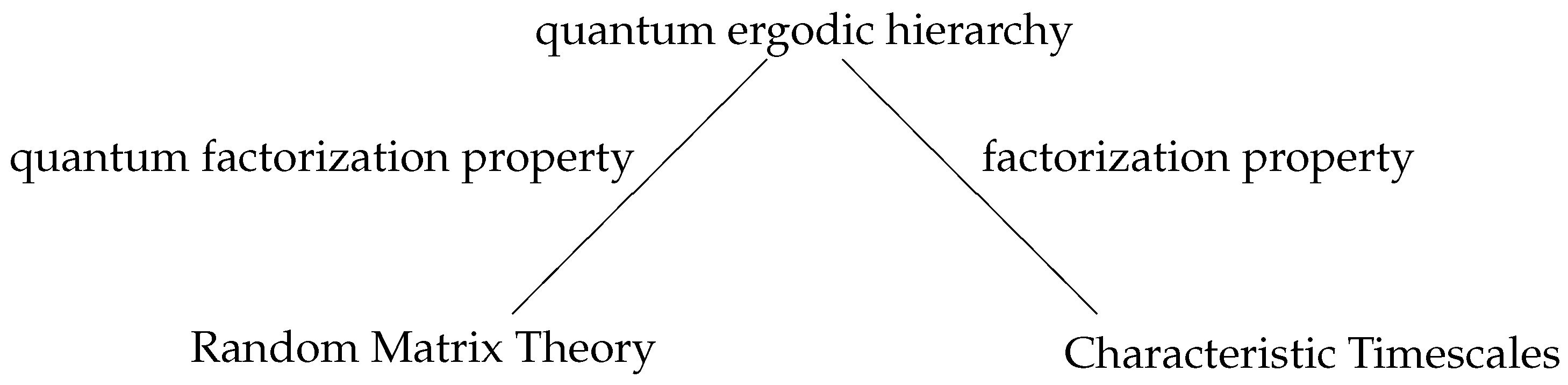
© 2017 by the authors. Licensee MDPI, Basel, Switzerland. This article is an open access article distributed under the terms and conditions of the Creative Commons Attribution (CC BY) license (http://creativecommons.org/licenses/by/4.0/).
Share and Cite
MDPI and ACS Style
Gomez, I.S.; Losada, M.; Lombardi, O. About the Concept of Quantum Chaos. Entropy 2017, 19, 205. https://doi.org/10.3390/e19050205
AMA Style
Gomez IS, Losada M, Lombardi O. About the Concept of Quantum Chaos. Entropy. 2017; 19(5):205. https://doi.org/10.3390/e19050205
Chicago/Turabian StyleGomez, Ignacio S., Marcelo Losada, and Olimpia Lombardi. 2017. "About the Concept of Quantum Chaos" Entropy 19, no. 5: 205. https://doi.org/10.3390/e19050205
Note that from the first issue of 2016, this journal uses article numbers instead of page numbers. See further details here.