
Information Content Based Optimal Radar Waveform Design: LPI’s Purpose

Key Laboratory of Radar Imaging and Microwave Photonics (Ministry of Education), Nanjing University of Aeronautics and Astronautics, Nanjing 210016, China
*
Author to whom correspondence should be addressed.
Entropy 2017, 19(5), 210; https://doi.org/10.3390/e19050210
Submission received: 26 March 2017
/
Revised: 30 April 2017
/
Accepted: 3 May 2017
/
Published: 6 May 2017
(This article belongs to the Section Information Theory, Probability and Statistics)
Abstract
:This paper presents a low probability of interception (LPI) radar waveform design method with a fixed average power constraint based on information theory. The Kullback–Leibler divergence (KLD) between the intercept signal and background noise is presented as a practical metric to evaluate the performance of the adversary intercept receiver in this paper. Through combining it with the radar performance metric, that is, the mutual information (MI), a multi-objective optimization model of LPI waveform design is developed. It is a trade-off between the performance of radar and enemy intercept receiver. After being transformed into a single-objective optimization problem, it can be solved by using an interior point method and a sequential quadratic programming (SQP) method. Simulation results verify the correctness and effectiveness of the proposed LPI radar waveform design method.
1. Introduction
In the past, short duration pulse train waveforms are widely equipped with most military radars. These pulses have a high ratio of peak to average power without any frequency or phase modulations, and, therefore, can be easily detected by adversary intercept systems, such as electronic support measures (ESMs), electronic attack (EA) systems and radar warning receivers (RWRs), in modern battlefields [1,2,3]. For surviving these enemy attacks, complex radar waveforms are designed to reduce the detection performance of passive intercept receiver devices, which can eventually achieve that the radar detection range is greater than the enemy interception range. These radar waveforms are called low probability of interception (LPI) waveforms, which have been developed for several decades [1,2,3,4,5,6,7].
They employ wideband modulation techniques to spread their energy in frequency domain, so that the signal strength in each frequency bin can be effectively reduced. Available wideband modulation techniques include frequency modulation, phase modulation, pseudo-noise modulation and so on. They generate the most common LPI radar waveforms, such as linear frequency modulation (LFM) waveform, Frank code, P1–P4 codes, Costas code and frequency shift keying/phase shift keying (FSK/PSK) signal [7]. However, the design of these waveforms does not consider optimal or near-optimal radar performance. Actually, LPI waveform design is a trade-off between radar task performance (such as detection performance, identification performance, location performance, etc.) and LPI performance. One extreme is a waveform with optimal radar performance which completely ignores its LPI performance, while the other extreme gives full consideration of the worst detection performance of enemy intercept receiver without regard to radar performance. The ideal LPI waveform would be to both achieve high radar performance while maintaining its LPI performance. Due to the fact that radar can obtain an additional matched filtering gain with prior information about its transmitted waveform, while the adversary intercept receiver can only capture fewer processing gains by using time-frequency analyses as it has no information about the received signals, the ideal LPI radar waveform can be achievable in practice by making a small reduction of radar performance but a sharply shrinkage of interception performance of adversary intercept receiver.
In this paper, we hope to model and solve the trade-off. To achieve it, the first question is the establishment of separate optimization metrics for radar and the intercept receiver. Many metrics about optimal radar performance have been proposed, such as mutual information (MI), output signal-to-noise ratio (SNR), mean square error and so on [8,9,10,11,12,13,14]. Therein, the maximization of MI has been widely employed in radar waveform design [8,9,10]. However, the performance metrics of the intercept receiver for radar waveform design are rarely studied. The existing LPI waveform ranking metrics include time-bandwidth product, peak to average power ratio [1,2,15,16] and their integrated function [17]. In 2015 and 2016, we presented simpler and more effective LPI ranking metrics [18,19] from the perspective of information distance via ignoring the concrete form of radar waveforms. Based on these metrics, in this paper, we treat the Kullback–Leibler divergence (KLD) between the intercept signal and background noise as a practical performance metric of intercept receiver for LPI radar waveform design. Therefore, based on maximizing MI of radar and minimizing KLD of intercept receiver, an LPI waveform design method is presented and solved under the constraint of a fixed average transmitted power. The simulation results verify its correctness and effectiveness.
The rest of this paper is organized as follows. In Section 2, the MI of radar and KLD of intercept receiver are analyzed, respectively. In Section 3, the optimization model of LPI radar waveform design is developed. In addition, its solution is introduced via using the interior point method and the sequential quadratic programming (SQP) method in combination. In Section 4, the performance of the proposed LPI radar waveform design method is evaluated. Conclusions are drawn in Section 5.
2. Information Theoretic Analyses of Radar and Intercept Receiver
2.1. Mutual Information in Radar System
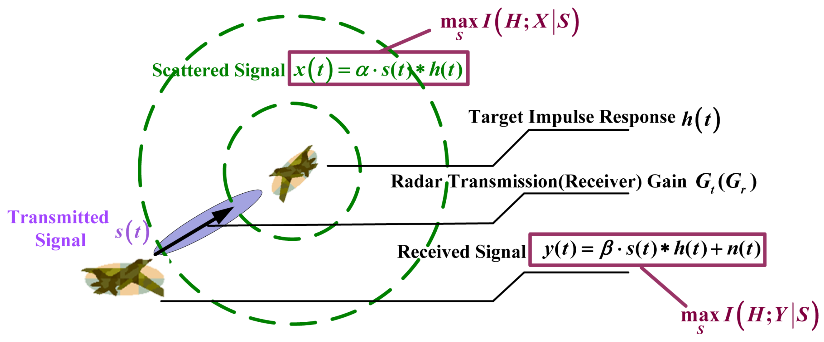
We begin with a brief overview of Bell’s MI in the radar system [9], which, in this paper, is used as the radar performance metric in LPI radar waveform design. The task of radar is to obtain information about targets, which will be probed by the transmitted waveforms. It can be depicted by Figure 1. Radar waveform is emitted by the transmitting antenna with gain in the target direction. Then, it can be intercepted and scattered by the target with a target impulse response . The scattered waveform can be expressed as
where, denotes energy attenuation coefficient, which is a function of emitter wavelength , antenna gain , propagation distance R, path loss and target impulse response , which is assumed as a zero-mean Gaussian random process, and the symbol denotes convolution. After propagating in the atmosphere, the scattered waveform can be captured by the radar receiving antenna with gain . Due to the existence of additive noise in the propagation path and radar receiver, the received signal is a noisy signal. It can be expressed as
where is a zero-mean additive white Gaussian noise. Similar to the definition of , is also an energy attenuation coefficient related to receiving antenna gain , propagation distance R and path loss , and .
For notation convenience, , , and are denoted as the discrete transmitted waveform, scattered waveform, received waveform and additive white Gaussian noise, respectively. The more amount of information about the target impulse response the scattered waveform contains, the more information about the target the radar system will obtain to better detect, locate, identify and track the target. Hence, the waveform optimization problem can be described as
According to Equation (1), the scattered waveform is a Gaussian random process with zero mean and variance , which is independent with zero-mean additive white Gaussian noise with variance . Hence, the received waveform is also a Gaussian random process with zero mean and variance . and are also assumed to be statistically independent. The optimization problem in Equation (3) can be converted to maximize the mutual information between the random target impulse response and the received waveform . Since Bell has proved that the waveforms that maximize also maximize , the waveform optimization problem can be recast as [9]
As described in [9], the transmitted waveform is considered as a finite energy deterministic waveform with energy and duration , and the bandwidth of is subject to the operation bandwidth of the radar system. For the convenience of analysis, the frequency interval is split into a large number of sufficiently small and disjoint sub-bands, whose bandwidth is , and , , , denote the components of , , , with frequencies in the k-th sub-band.
By transforming the in Equation (1) from time domain to frequency domain, we have , where , and are frequency domain representations of , and , and . The mutual information in each sub-band can be calculated as
where is the one-sided power spectral density of Gaussian noise of radar.
Let , the mutual information is an integral of over the frequency band ,
2.2. Kullback–Leibler Divergence in the Intercept Receiver
Suppose the target is equipped with an intercept receiver. When the radar signal is used to detect the target, it can also be intercepted by intercept receiver, which makes the radar face serious threats, such as anti-radiation missiles. Therefore, the transmitted waveform should be designed to reduce the detection and identification probabilities of the intercept receiver. It can be depicted in Figure 2. After being radiated by the radar emitting antenna and propagated in the atmosphere, the radar waveform can be intercepted by the intercept receiver. The intercept signal can be written as
where
wherein denotes the intercept receiver antenna gain.
After time-frequency characteristics are analyzed, the intercept signal is detected and extracted features to recognize its modulation type for achieving the emitter location and recognizing the emitter. Since it is a common view that white noise is the best LPI waveform, the closer the distance between intercept signal and noise signal is, the more difficult it is to detect and recognize the intercept signal. It is logical to compare random data sets by ways of the associated probability density function (PDF). The waveform optimization problem against intercept receiver can be briefly written as
where and are the PDFs of intercept signal and noise signal , and denotes a distance measure.
There are many PDF distance measures to quantify the disparity between PDFs [20], such as norm, Kullback–Leibler divergence (KLD), Bhattacharyya distance, f-divergence, Hellinger distance, etc. Among these distance measures, KLD has been confirmed to be a powerful and accurate tool to measure the information of multivariate data with lower complexity and superior performance [21]. Thus, we use KLD here as the PDF distance measure, which is denoted as .
In the frequency domain, the intercept signal in Equation (7) can be transformed as , where , and are frequency domain representations of signals , and . Like the computation of Bell’s MI, we also split the frequency interval into a large number of sufficiently small and disjoint frequency intervals whose bandwidth is , and for all , we have , where # can be the waveforms , and . In addition, denotes the component of with frequencies in , which is the same for and .
In each frequency interval , we suppose the sample frequency is according to the sampling theory, and, therefore, the sample sizes of , , and are . Since the distribution of background noise of the intercept receiver at the frequency is a normal distribution with zero mean and variance , which can be denoted as , the distribution of the intercept signal at the frequency can be achieved as , where
where is the one-sided power spectral density of Gaussian noise of intercept receiver.
We can calculate the KLD between and ,
The KLD in Equation (11) is a function of signal-to-noise ratio (SNR) at the frequency . The lower SNR a waveform possesses in each frequency, the harder it is for the intercept receiver to detect it. It meets our common knowledge and experience. The waveform optimization problem against intercept receiver then can be described as the minimization of the KLD in each frequency . In order to facilitate the solving of the optimization problem, the natural exponential function of the KLD is used as the new objective function, which can be denoted as . Since the constructed KLD has the same monotonicity about with the KLD in Equation (11), minimization is also minimization .
Since the sample size in each frequency interval is , the KLD between the component and is
When , the KLD is an integral of over the frequency band ,
3. Optimization of Radar Waveform for the Purpose of LPI
According to the analysis of Section 2, the mutual information and the KLD are tied to the radar and the intercept receiver performance, respectively. We need a transmitted waveform should not only have good performance of detecting, locating, identifying and tracking target, but also have a good LPI performance against the detection and identification of intercept receiver. Here, the process of LPI radar waveform design can be described as the following optimization problem:
where is the average transmitted power and is fixed.
To maximize the radar performance is just one part of the job in radar waveform design, and the minimization of the performance of the intercept receiver should also be taken into account, as shown in Equation (14), which is a multi-objective optimization problem with respect to under a fixed average power constraint. However, the primary task of the emitting waveform is to fulfill the target detection. The designed waveform should be considered the LPI capability under the condition of meeting radar performance. Thus, the multi-objective optimization problem in Equation (14) can be simplified to a single-objective optimization problem, that is,
where is the needed mutual information to meet the radar performance, which can be set at various values in different battling scenarios.
The maximization of the mutual information of radar and the minimization of the KLD of intercept receiver are just like lance and shield. To solve the problem, we minimize the KLD in the situation that the mutual information makes some concessions, as shown in Equation (15). Before solving the optimization problem, we first digress to discuss the solutions of two independent optimization problems, which take the mutual information and the KLD as objective functions, respectively. The two optimization problems are expressed as
3.1. Solution of the OP1
For OP1, Bell has given the concrete solving process [9]. For comparing with the solving process of OP2 and determing the constraint value easily, we restate the process briefly.
The Lagrange multiplier technique is utilized here, and the objective function can be yielded as
Taking the partial derivative of with respect to and setting it to zero, we have
Since the partial derivative of with respect to is less than zero, the combined solution of Equation (19) and the constraint , which maximizes the mutual information , can be written as
where is a constant, and the value of A can be solved numerically by a search algorithm to satisfy the constraint .
The maximum value of the mutual information can be achieved as
Thus, the constraint value of MI should satisfy .
3.2. Solution of the OP2
Like the solving method of OP1, we reuse the Lagrange multiplier technique, and the objective function can be obtained as
This is seen to be equivalent to minimizing for each frequency , where is given by
Taking the partial derivative of with respect to and setting it to zero, we have
Solving for , we have
where is a constant.
Substituting the in Equation (25) into the constraint , we have
Since the partial derivative of with respect to is greater than zero, the solution in Equation (25) can minimize the KLD , which can be written as
When the background noise of intercept receiver is a white Gaussian noise, the power spectral density is a constant. Under this assumption, the optimized waveform that minimizes is
From the Equation (28), we have a conclusion that it is most difficult to intercept the transmitted waveform whose power is distributed equally in the whole bandwidth for an intercept receiver under the assumption of white Gaussian noise.
Since the radar has no information about the background noise types of unknown intercept receivers, the assumption of white Gaussian noise is the most reasonable choice. Moreover, the background noise in most of the receivers is white Gaussian noise. Here, it is unnecessary to study the solution of OP2 under the assumption of colored Gaussian noise. In this case, we only need to add another constraint , and the interior point method can be used to solve the optimization problem. Here, the solving process about colored Gaussian noise will not be described in detail. The corresponding experiment results will be presented in Section 4.
3.3. Solution for the Optimization Problem of LPI Waveform Design
We now give the detailed solving process of the optimization problem in Equation (15). In order to achieve the optimal solution smoothly, the discrete form of the optimization problem first need to be obtained, which can be written as
where are the uniform partition points in the frequency interval , , and .
The classical method for solving the nonlinear optimization problem in Equation (29) is the combination of interior point method and sequential quadratic programming (SQP) method [22]. Through introducing slack variables , the inequality constraints in Equation (29) can be transformed into equality constraints, and correspondingly bounds are yielded. The transformed optimization problem can be described as
According to the interior point method, the barrier function can be constructed as
By introducing a penalty factor , the optimization problem in Equation (30) can be rewritten as
Here, the SQP method can be applied to the optimization problem in Equation (32) and yields the quadratic program
where , ,
Considering the possibility of indefiniteness of , Richard H. Byrd uses a trust region method to solve such problems [22]. The optimization problem can be recast as
where denotes a norm, and denotes a trust region radius, which will be updated in each iteration.
Here, we uses the algorithm proposed by Richard H. Byrd [22] to solve our optimization problem of Equation (29). The algorithmic framework of LPI radar waveform design is briefly introduced below (See Algorithm 1). Details of the nonlinear programming algorithm can be found in [22].
| Algorithm 1: Radar waveform optimization for the purpose of LPI |
|
4. Simulation Results
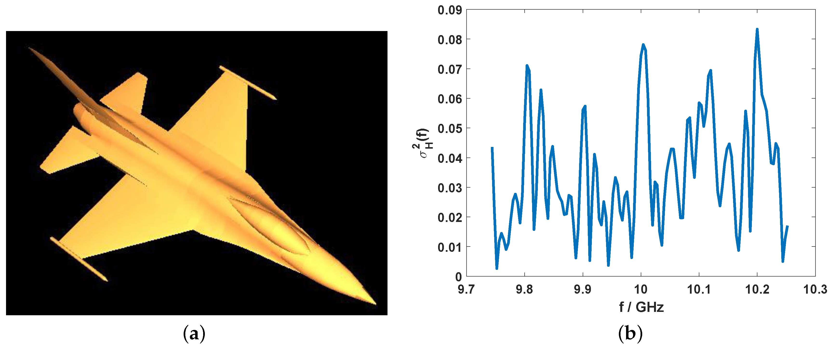
In this section, several simulation experiments are provided to verify the effectiveness of the proposed LPI radar waveform design method, which considers not only the maximization of radar performance, but also the minimization of intercept receiver performance. The simulation parameters are listed in Table 1. The background noise in simulations includes white Gaussian noise and colored Gaussian noise. The one-side power spectral density of white Gaussian noise is . The one-side power spectral density of colored Gaussian noise is a sinc function, which is set as , for frequencies GHz. For target information, we suppose the target headed for radar is F-16 aircraft, which is modeled in Figure 3a, and the variance GHz of its impulse response with azimuth and elevation between the radar and the target has been calculated by electromagnetism simulation software, which is shown in Figure 3b. We also compare the proposed optimized radar waveforms with the common LPI radar waveforms: LFM, Frank and P1-P4 codes. Their transmit power, bandwidth and duration are the same as those of optimized waveforms, and the code numbers of Frank, P1–P4 codes are 64.
To test the proposed LPI waveform design method, we run four experiments, including both radar and intercept receiver, are under a white Gaussian noise background, only radar is under a colored Gaussian noise, only the intercept receiver is under a colored Gaussian noise, and both radar and intercept receiver are under a colored Gaussian noise. In each experiment, the SNR losses, which are defined in Equation (36), of radar and the intercepter receiver are simulated, respectively, as a metric of performance degradation. Through comparing the SNR losses of radar and intercepter receiver, the superiority of our proposed LPI waveform design method can be judged easily:
where is the difference between the receiving SNR of the optimized waveform just considering the maximization of radar performance and the receiving SNR of the proposed optimized waveform.
4.1. Both Radar and Intercept Receiver are under White Gaussian Noise Background
Figure 4a shows the optimized waveforms with different mutual information constraints used our proposed MI-KLD method, and the optimized waveforms used the methods of maximization of radar performance (see OP1) and minimization of intercept receiver performance (see OP2). As a result of the comparison with Figure 3b, the optimized waveform (see the dotted purple line in Figure 4a) of OP1 has a large value of power spectral density at the frequencies where the variance of the target impulse response also has a larger value to get the maximum matching with the target, so that the radar can achieve the best performance. However, due to the restriction of a limited transmit power , the power spectral density of the optimized waveform is equal to zero at most of frequencies where the variance of the target impulse response has a relatively low value, which can be verified by Equation (20). For the solution (see the dotted red line in Figure 4a) of OP2, the power of the optimized waveform is equally distributed into all frequencies to decrease the intercept probability at each frequency, so that the intercept receiver can have a worst performance.
The aim of the proposed LPI waveform design method is to reduce the peak power under the condition of a certain loss of target matching quality. The reduction of peak power is to decrease the interception probability of intercept receivers, and the loss of the target matching quality means the degradation of radar performance. The blue line in Figure 4a shows that the optimized waveform, to a certain extent, not only achieves the target matching, but also realizes the reduction of peak power. With the shrinkage of the constraints of mutual information, the target matching quality and peak power of the optimized waveform keeps coming down, and the optimized waveform tends to the solution of OP2. The comparison of the performance degration between radar and intercept receiver with the reduction of is shown in Figure 4b.
Since the radar has the prior information about its transmitted waveform, it can increase the receiving SNR through the matched filtering technique. Thus, a certain loss of target matching quality may have little impact on the receiving SNR of radar. However, the intercept receiver has no information about the receiving waveform. It can only detect the receiving signal by the signal power in each frequency, so a certain reduction of peak power may have a serious effect on the receiving SNR of intercept receivers. These can be verified by the simulation results in Figure 4b. When the constraints of mutual information is , which is close to the maximum value of mutual information calculated by Equation (21), the SNR reduction for radar is dB, while the SNR reduction is dB for intercept receiver. In addition, the gap between the SNR loss of radar and the SNR loss of intercept receiver keeps increasing with the relaxation of mutual information constraint until , where the SNR losses of radar and intercept receiver are dB and dB, respectively. As , the optimized waveform is the solution of OP2, which is the red line displayed in Figure 4a, and the SNR losses of both radar and intercept receiver remain unchanged. From Figure 4b, we find that the performance of intercept receiver can be degraded sharply, while the performance of radar has a small reduction. Thus, the optimized waveform has a significant LPI performance.
Compared with the common LPI radar waveforms, our designed waveforms still have a significant LPI superiority, as shown in Table 2. For each compared LPI radar waveform (LFM, Frank, P1-P4), we can find an optimized waveform from different MI constraint values, whose SNR loss of radar is equal to (or less than (since the maximal SNR loss of radar is dB for optimized waveforms)) that of the compared waveform, as the second row shows. However, the SNR losses of intercept receiver are different between each compared waveform and its corresponding optimized waveform. As each column of the third row shows, the SNR loss of intercept receiver of each compared waveform is less than that of its corresponding optimized waveform. Thus, we can draw a conclusion that not only can our proposed optimized waveforms ensure the radar performance, but they can also maximize the performance degradations of intercept receiver.
4.2. Only Radar or Intercept Receiver is under a Colored Gaussian Noise Background
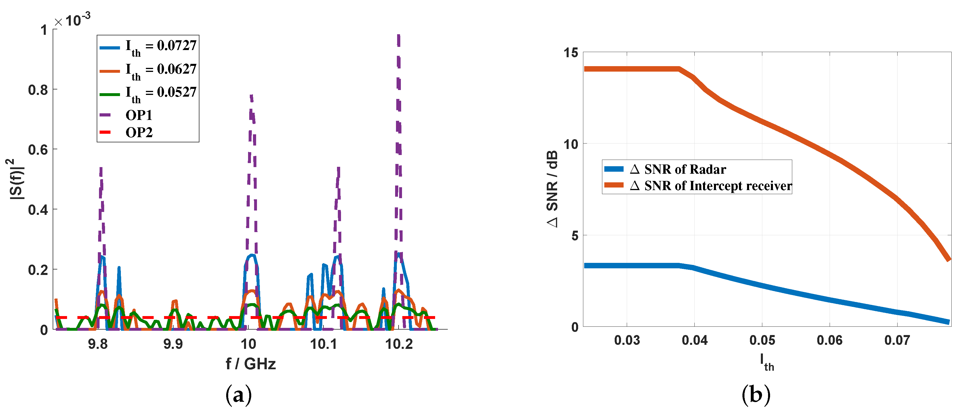
In Figure 5, we change the background noise of radar from white Gaussian noise to colored Gaussian noise. Since the power spectral density of the optimized waveform for OP1 is a function of (see Equation (20)), the power spectral density of the optimized waveform has a large value at the frequencies where has a large value and has a small value. Thus, the optimized waveform (see the dotted purple line in Figure 5a) of OP1 has an extra peak compared with the dotted purple line in Figure 4a. Due to the background noise of intercept receiver is still the white Gaussian noise, the optimized waveform of OP2 remains as a constant , and the optimized waveform of the proposed waveform design method tends to the constant with the reduction of the mutual information constraint . From Figure 5b, we find the gap between the SNR loss of radar and the SNR loss of intercept receiver is still huge. As there are such huge gaps, the optimized waveform can achieve a superior LPI performance.
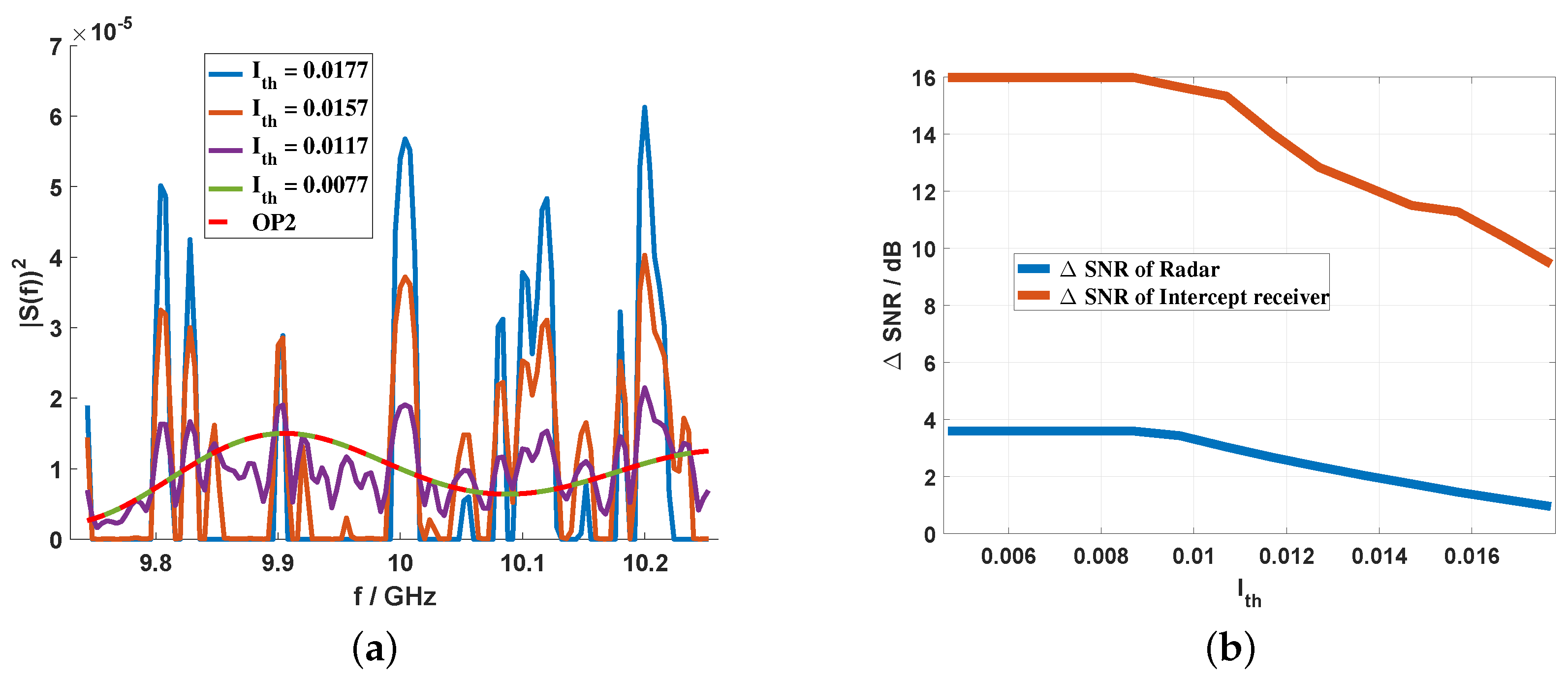
Figure 6a gives the optimized solutions of the proposed optimization problem under the assumption that the background noise of intercept receiver is a colored Gaussian noise. In order to better illustrate the changes of the optimized waveform in this case, we decrease the radar transmit power from 20 KW to 5 KW. Since the solution of OP2 is to make the SNR in each frequency of intercept receiver reach the minimum, it will match the given background noise of intercept receiver well, as the dotted red line shows in Figure 6a. Like the simulation results above, the target matching quality and peak power of the optimized waveform keeps coming down with the relaxing of the mutual information constraints , and the optimized waveform tends to the solution of OP2 eventually. As the Figure 6b shows, such descents have less impact on radar performance, while they hit performance of the intercept receiver hard. The SNR losses of intercepter receiver are above 8 dB and finally reach 17 dB, while the SNR losses of radar keep within 4 dB. Thus, the optimized waveforms in a colored Gaussian noise still have a preferable LPI performance.
Table 3 gives the comparison of SNR losses between the common LPI radar waveforms and our optimized waveforms in the case that the background noise of radar is a colored Gaussian noise; meanwhile, Table 4 gives that in the case that the background noise of intercept receiver is a colored Gaussian noise. Both Table 3 and Table 4 show our designed waveforms can further reduce the performance of intercept receiver with almost the same radar performance, compared with common LPI radar waveforms. For example, in Table 3, we find the SNR losses dB of radar for waveforms Frank, P1, P3, P4, are more than the maximal SNR loss dB for optimized waveforms. Although the difference is small, the SNR loss of intercept receiver of optimized waveforms is about 3 dB higher than that of compared waveforms. Therefore, the LPI performance of our designed waveforms is more superior to the common LPI radar waveforms.
4.3. Both Radar and Intercept Receiver are under Colored Gaussian Noise
In this subsection, we suppose both the background noises of radar and the intercept receiver are colored Gaussian noise. For better illustrating the changes of the optimized waveforms with the simulation results above, we still reduce the power of transmit waveform from 20 KW to 5 KW. The optimized waveforms should be the combination of the waveforms displayed in Figure 5a and Figure 6a. When the constraints of mutual information are strong, which means is close to the maximum mutual information, the optimized waveform should be similar to the corresponding waveforms in Figure 5a. Conversely, as there are almost no constraints of mutual information, that is has a smaller value than the maximum mutual information, the optimized waveform is the solution of OP2, as the dotted red lines show in Figure 6a and Figure 7b. For other values of , the optimized waveforms should not only have a certain target () matching quality, but also be around the solution of OP2, as the purple line shows in Figure 7a. For the comparison between the performance degradations of radar and intercepter displayed in Figure 7b, we still find the SNR losses of intercepter receiver are above 9 dB and finally reach 16 dB, while the SNR losses of radar only keep within 4 dB. Thus, the optimized waveforms on the condition that both radar and intercept receiver are under colored Gaussian noise still have a predominant LPI performance. The comparative results in Table 5 also verify this conclusion, since the optimized waveforms can reduce more performance of the intercept receiver with the same performance loss of radar.
5. Conclusions
In response to the LPI requirement of modern military radar, waveforms with a fixed average power constraint have been designed in this paper to minimize the interception performance of enemy receivers under the condition of meeting a specified radar performance. In other words, the aim of the proposed LPI radar waveform design method is to reduce the peak power as much as possible under the condition of a certain loss of target matching quality. During the modeling of LPI waveform design, the MI between scattered waveform and radar received waveform is treated as a performance metric of radar, and for enemy receiver, the KLD between intercepted waveform and background noise is presented as its performance metric. Simulation results show that the proposed LPI waveform design method is correct and effective. A certain loss of target matching quality has little impact on radar performance, while a certain reduction of peak power has a serious effect on the performance of enemy receivers. The huge gap of performance loss between radar and intercept receiver is the significance of the proposed LPI waveform design method.
Acknowledgments
This work is supported by the National Natural Science Foundation of China (Grant No. 61371170), the Fundamental Research Funds for the Central Universities (Grant No. NP2015404, No. NS2016038), the Aeronautical Science Foundation of China (Grant No. 20152052028) and the Funding of Jiangsu Innovation Program for Graduate Education (Grant No. KYLX15_0282). The authors are grateful to the anonymous reviewers for their constructive comments on the paper.
Author Contributions
Jun Chen and Jianjiang Zhou contributed to the establishment of the LPI waveform design model; Jun Chen and Fei Wang solved the optimization problem; Fei Wang performed the experiments; Jun Chen wrote the paper; and all of the authors have read and approved the manuscript.
Conflicts of Interest
The authors declare no conflict of interest.
References
- David, L.J. Introduction to stealth systems. In Introduction to RF Stealth; SciTec Publishing Inc.: Raleigh, NC, USA, 2004; pp. 1–59. [Google Scholar]
- Schleher, D.C. LPI radar: Fact or fiction. IEEE Aerosp. Electron. Syst. Mag. 2006, 21, 3–6. [Google Scholar] [CrossRef]
- Wang, F.; Li, H.; Xia, W.; Zhou, J. LPI Airborne Radar Signal Processing; Science Press: Beijing, China, 2015; pp. 1–19. [Google Scholar]
- Stove, A.G.; Hume, A.L.; Baker, C.J. Low probability of intercept radar strategies. IEE Proc. Radar Sonar Navig. 2004, 151, 249–260. [Google Scholar] [CrossRef]
- Schrick, G.; Wiley, R.G. Interception of LPI radar signals. In Proceedings of the IEEE International Conference on Radar, Arlington, VA, USA, 7–10 May 1990; pp. 108–111. [Google Scholar]
- Van der Merwe, J.R.; du Plessis, W.P.; Maasdorp, F.D.; Cilliers, J.E. Introduction of low probability of recognition to radar system classification. In Proceedings of the IEEE International Conference on Radar, Philadelphia, PA, USA, 2–6 May 2016; pp. 1–5. [Google Scholar]
- Pace, P.E. Detecting and Classifying Low Probability of Intercept Radar, 2nd ed.; Artech House: Norwood, MA, USA, 2009; pp. 81–247. [Google Scholar]
- Gini, F.; De Maio, A.; Patton, L. Waveform Design and Diversity for Advanced Radar Systems; IET Radar and Sonar Navigation: London, UK, 2011. [Google Scholar]
- Bell, M.R. Information theory and radar waveform design. IEEE Trans. Inf. Theory 1993, 39, 1578–1597. [Google Scholar] [CrossRef]
- Yang, Y.; Blum, R.S. MIMO radar waveform design based on mutual information and minimum mean-square error estimation. IEEE Trans. Aerosp. Electron. Syst. 2007, 43, 330–343. [Google Scholar] [CrossRef]
- Aubry, A.; De Maio, A.; Farina, A.; Wicks, M. Knowledge-aided (potentially cognitive) transmit signal and receive filter design in signal dependent clutter. IEEE Trans. Aerosp. Electron. Syst. 2013, 49, 93–117. [Google Scholar] [CrossRef]
- Aubry, A.; De Maio, A.; Naghsh, M. MIMO radar waveform design based on mutual information and minimum mean-square error estimation. IEEE J. Sel. Topics Signal Process. 2015, 9, 1387–1399. [Google Scholar] [CrossRef]
- Zhou, W.; Fei, M.; Zhou, H.; Li, K. A sparse representation based fast detection method for surface defect detection of bottle caps. Neurocomputing 2014, 123, 406–414. [Google Scholar] [CrossRef]
- Zhou, H.; Yuan, Y.; Lin, F.; Liu, T. Level set image segmentation with Bayesian analysis. Neurocomputing 2008, 71, 1994–2000. [Google Scholar] [CrossRef]
- Chen, Z.M. Stealth Waveform for Airborn Radar. Modern Radar 2006, 9, 1–7. [Google Scholar]
- Wang, F.; Sellathurai, M.; Liu, W.; Zhou, J. Security information factor based airborne radar RF stealth. J. Syst. Eng. Electron. 2015, 26, 258–266. [Google Scholar] [CrossRef]
- Fancey, C.; Alabaster, C.M. The metrication of low probability of intercept waveforms. In Proceedings of the IEEE International Conference on Waveform Diversity and Design (WDD), Niagara Falls, ON, Canada, 8–13 August 2010; pp. 58–62. [Google Scholar]
- Chen, J.; Wang, F.; Zhou, J. The metrication of LPI radar waveforms based on the asymptotic spectral distribution of wigner matrices. In Proceedings of the IEEE International Symposium Information Theory (ISIT), Hong Kong, China, 14–19 June 2015; pp. 331–335. [Google Scholar]
- Chen, J.; Wang, F.; Zhou, J.; Dai, C. Information content-based low probability of interception waveforms selection against channelized receivers. In Proceedings of the International Symposium Signal, Image, Video and Communications (ISIVC), Tunis, Tunisia, 21–23 Novmber 2016; pp. 115–119. [Google Scholar]
- Cha, S.H. Comprehensive survey on distance/similarity measures between probability density functions. Int. J. Math. Models Methods Appl. Sci. 2007, 4, 300–307. [Google Scholar]
- Tumminello, M.; Lillo, F.; Mantegna, R. N. Kullback–Leibler distance as a measure of the information filtered from multivariate data. Phys. Rev. E 2007, 76, 1–12. [Google Scholar] [CrossRef] [PubMed]
- Byrd, R.H.; Gilbert, J.C.; Nocedal, J. A trust region method based on interior point techniques for nonlinear programming. Math. Program. 2000, 89, 149–185. [Google Scholar] [CrossRef]
Figure 1.
Radar radiation diagram.

Figure 2.
Interception diagram of enemy receiver.
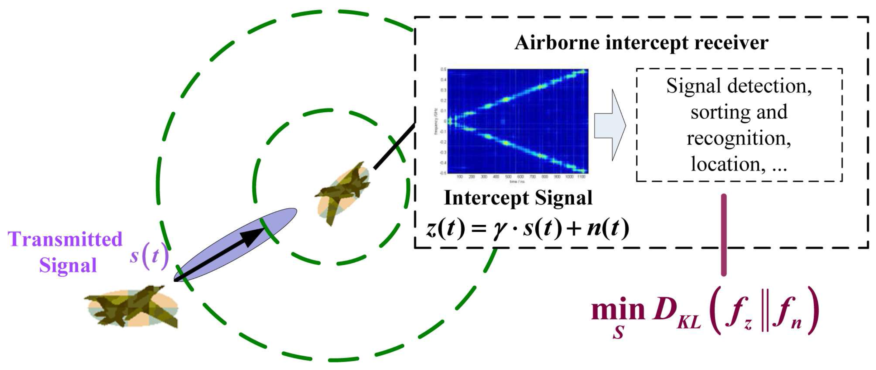
Figure 3.
(a) model of F-16 aircraft; (b) variance of F-16 impulse response with frequencies GHz and azimuth , elevation between the radar and the target F-16.
Figure 3.
(a) model of F-16 aircraft; (b) variance of F-16 impulse response with frequencies GHz and azimuth , elevation between the radar and the target F-16.

Figure 4.
(a) optimized waveforms of the proposed mutual information and Kullback–Leibler divergence (MI-KLD) based method with different mutual information constraints , and optimized waveforms of OP1 and OP2; (b) performance reductions of radar and intercept receiver versus the reduction of (both radar and intercept receiver are under white Gaussian noise background and average transmitted power KW).
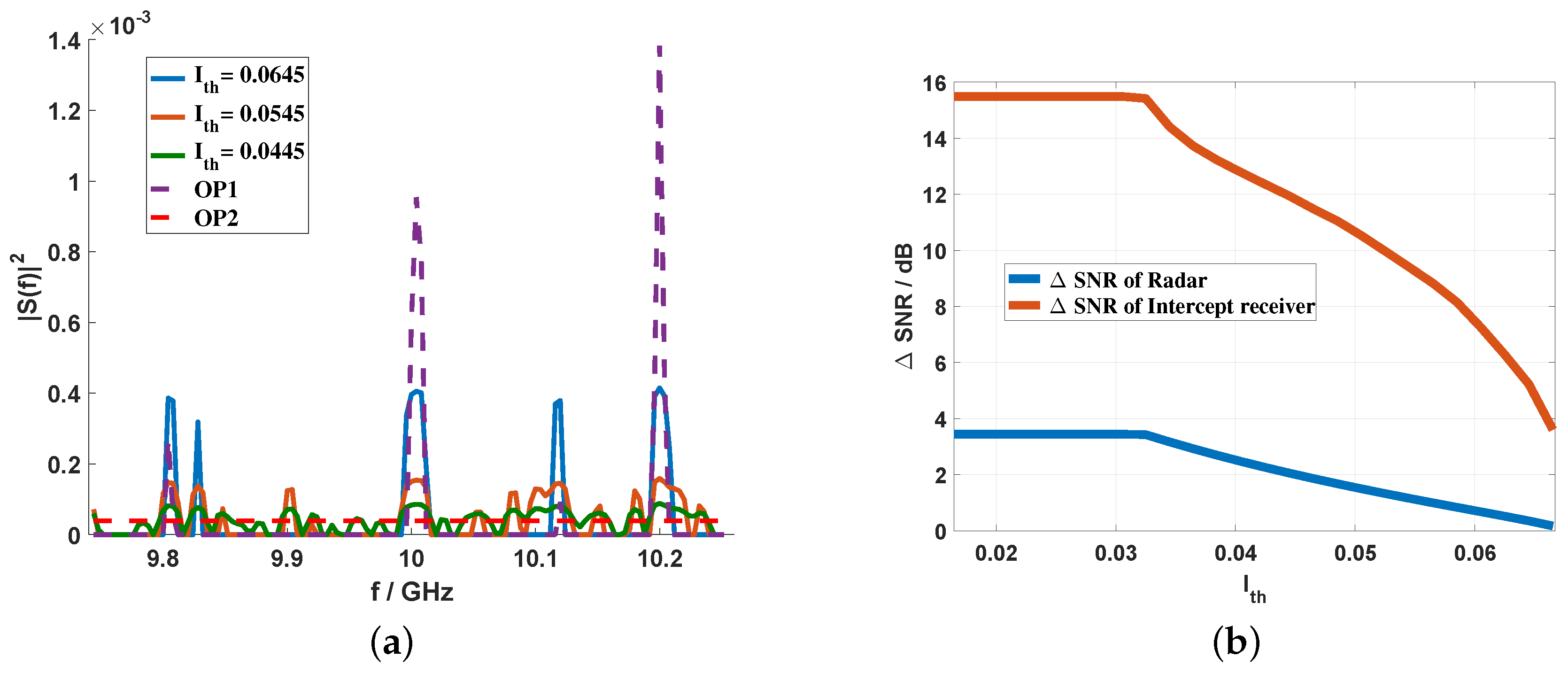
Figure 5.
(a) optimized waveforms of the proposed MI-KLD method with different mutual information constraints , and optimized waveforms of OP1 and OP2; (b) performance reductions of radar and intercept receiver versus the reduction of (the background noise of radar is a colored Gaussian noise, while the intercept receiver is under the white Gaussian noise background and average transmitted power KW).

Figure 6.
(a) optimized waveforms of the proposed MI-KLD method with different mutual information constraints , and optimized waveforms of OP2; (b) performance reductions of radar and intercept receiver versus the reduction of (the background noise of the intercept receiver is a colored Gaussian noise, while the radar is under white Gaussian noise background and average transmitted power KW).

Figure 7.
(a) optimized waveforms of the proposed MI-KLD method with different mutual information constraints , and optimized waveforms of OP2; (b) performance reductions of radar and intercept receiver versus the reduction of (both radar and intercept receiver are under a colored Gaussian noise background and average transmitted power KW).


Table 1.
Simulation parameters.
| Parameter Name | Parameter Value | Parameter Name | Parameter Value |
|---|---|---|---|
| Radar transmitting antenna gain | 30 dB | Radar Receiving antenna gain | 30 dB |
| Intercept receiver antenna gain | 0 dB | emitter wavelength | 0.03 m |
| Waveform bandwidth | 512 MHz | Waveform duration | 25 ns |
| Average transmitted power | 20 KW | Path loss | −10 dB |
| Path loss | −10 dB | Detection distance R | 100 Km |
Table 2.
Signal-to-noise ratio (SNR) losses for the common low probability of interception (LPI) radar waveforms and optimized waveforms (Both radar and intercept receiver are under white Gaussian noise background and average transmitted power KW).
Table 2.
Signal-to-noise ratio (SNR) losses for the common low probability of interception (LPI) radar waveforms and optimized waveforms (Both radar and intercept receiver are under white Gaussian noise background and average transmitted power KW).
| LFM OW | Frank OW | P1 OW | P2 OW | P3 OW | P4 OW | |
|---|---|---|---|---|---|---|
| of radar (dB) | 3.1150 | 3.4526 | 3.4526 | 3.4096 | 3.4526 | 3.4526 |
| 3.1150 | 3.4450 | 3.4450 | 3.4096 | 3.4450 | 3.4450 | |
| of intercept receiver (dB) | 4.5985 | 12.4808 | 12.4808 | 11.4856 | 12.4808 | 12.4808 |
| 14.0591 | 15.4911 | 15.4911 | 14.3828 | 15.4911 | 15.4911 |
Linear Frequency Modulation; Optimized Waveform (bold text).
Table 3.
SNR losses for the common LPI radar waveforms and optimized waveforms (the background noise of radar is a colored Gaussian noise, while the intercept receiver is under white Gaussian noise background and average transmitted power KW).
Table 3.
SNR losses for the common LPI radar waveforms and optimized waveforms (the background noise of radar is a colored Gaussian noise, while the intercept receiver is under white Gaussian noise background and average transmitted power KW).
| LFM OW | Frank OW | P1 OW | P2 OW | P3 OW | P4 OW | |
|---|---|---|---|---|---|---|
| of radar (dB) | 2.9966 | 3.3342 | 3.3342 | 3.2912 | 3.3342 | 3.3342 |
| 2.9966 | 3.3266 | 3.3266 | 3.2912 | 3.3266 | 3.3266 | |
| of intercept receiver (dB) | 3.1807 | 11.0629 | 11.0629 | 10.0678 | 11.0629 | 11.0629 |
| 12.6468 | 14.0732 | 14.0732 | 13.8503 | 14.0732 | 14.0732 |
Optimized Waveform (bold text).
Table 4.
SNR losses for the common LPI radar waveforms and optimized waveforms (the background noise of intercept receiver is a colored Gaussian noise, while the radar is under white Gaussian noise background, and average transmitted power KW).
Table 4.
SNR losses for the common LPI radar waveforms and optimized waveforms (the background noise of intercept receiver is a colored Gaussian noise, while the radar is under white Gaussian noise background, and average transmitted power KW).
| LFM OW | Frank OW | P1 OW | P2 OW | P3 OW | P4 OW | |
|---|---|---|---|---|---|---|
| of radar (dB) | 3.3256 | 3.6632 | 3.6632 | 3.6203 | 3.6632 | 3.6632 |
| 3.3256 | 3.6632 | 3.6632 | 3.6203 | 3.6632 | 3.6632 | |
| of intercept receiver (dB) | 7.8518 | 15.8298 | 15.8298 | 14.8673 | 15.8298 | 15.8298 |
| 16.8611 | 17.4032 | 17.4032 | 17.3344 | 17.4032 | 17.4032 |
Optimized Waveform (bold text).
Table 5.
SNR losses for the common LPI radar waveforms and optimized waveforms (both radar and intercept receiver are under a colored Gaussian noise background, and average transmitted power KW).
Table 5.
SNR losses for the common LPI radar waveforms and optimized waveforms (both radar and intercept receiver are under a colored Gaussian noise background, and average transmitted power KW).
| LFM OW | Frank OW | P1 OW | P2 OW | P3 OW | P4 OW | |
|---|---|---|---|---|---|---|
| of radar (dB) | 3.2133 | 3.5509 | 3.5509 | 3.5079 | 3.5509 | 3.5509 |
| 3.2133 | 3.5509 | 3.5509 | 3.5079 | 3.5509 | 3.5509 | |
| of intercept receiver (dB) | 6.3629 | 14.3410 | 14.3410 | 13.3782 | 14.3410 | 14.3410 |
| 15.4731 | 15.8928 | 15.8928 | 15.8032 | 15.8928 | 15.8928 |
Optimized Waveform (bold text).
© 2017 by the authors. Licensee MDPI, Basel, Switzerland. This article is an open access article distributed under the terms and conditions of the Creative Commons Attribution (CC BY) license (http://creativecommons.org/licenses/by/4.0/).
Share and Cite
MDPI and ACS Style
Chen, J.; Wang, F.; Zhou, J. Information Content Based Optimal Radar Waveform Design: LPI’s Purpose. Entropy 2017, 19, 210. https://doi.org/10.3390/e19050210
AMA Style
Chen J, Wang F, Zhou J. Information Content Based Optimal Radar Waveform Design: LPI’s Purpose. Entropy. 2017; 19(5):210. https://doi.org/10.3390/e19050210
Chicago/Turabian StyleChen, Jun, Fei Wang, and Jianjiang Zhou. 2017. "Information Content Based Optimal Radar Waveform Design: LPI’s Purpose" Entropy 19, no. 5: 210. https://doi.org/10.3390/e19050210
Note that from the first issue of 2016, this journal uses article numbers instead of page numbers. See further details here.