
On the Convergence and Law of Large Numbers for the Non-Euclidean Lp -Means

Space Science and Engineering, Southwest Research Institute, San Antonio, TX 78238, USA
Entropy 2017, 19(5), 217; https://doi.org/10.3390/e19050217
Submission received: 18 January 2017
/
Revised: 13 April 2017
/
Accepted: 9 May 2017
/
Published: 11 May 2017
Abstract
:This paper describes and proves two important theorems that compose the Law of Large Numbers for the non-Euclidean -means, known to be true for the Euclidean -means: Let the -mean estimator, which constitutes the specific functional that estimates the -mean of N independent and identically distributed random variables; then, (i) the expectation value of the -mean estimator equals the mean of the distributions of the random variables; and (ii) the limit of the -mean estimator also equals the mean of the distributions.
1. Introduction: Definition of -Means and Their Basic Properties
In [1,2,3], a generalized characterization of means was introduced, namely, the non-Euclidean means, based on metrics induced by -norms, wherein the median is included as a special case for () and the ordinary Euclidean mean for () (see also: [4,5]). Let the set of y-values (), associated with the probabilities ; then, the non-Euclidean means , based on -norms, are defined by
where the median and the arithmetic mean follow as special cases when the Taxicab and Euclidean -norms are respectively considered. Both the median and arithmetic means can be implicitly written in the form of Equation (1) as and (), respectively.
Note that the solution of Equation (1) is a specific case of the so-called M-estimators [6], while it is also related to the Fréchet Means [7]. The Euclidean norm is also known as “Pythagorean” norm. In [3], we preferred referring to the non-Pythagorean norms as non-Euclidean, inheriting the same characterization to Statistics. One may adopt the more explicit characterizations of “Non-Euclidean-normed” Statistics, for avoiding any confusion with the non-Euclidean metric of the (Euclidean-normed) Riemannian Geometry. As an example of an application in physics, the expectation value of an energy spectrum is defined by representing the non-Euclidean adaptation of internal energy [8].
Figure 1 illustrates an example of -means. We use the Poisson distribution and the dataset , for ; hence, the -means are implicitly given by (note that the constant term can be ignored). The function is examined for various values of the p-norm, either (a) super-Euclidean, , or (b) sub-Euclidean . The mean value for the Euclidean case, , is , which is represented by the diagonal line in both panels. We observe that for we always have , while for there is a critical value , for which for and for . The critical value increases with p, and as , . For , for any , while for , for any values of p.
The Law of Large Numbers is a theorem that guarantees the stability of long-term averages of random events, but is valid only for Euclidean metrics based on -norms. The purpose of this paper is to extend the theorem of the “Law of Large Numbers” to the non-Euclidean, -means. Namely, (i) the expectation value of the -mean estimator (that corresponds to Equation (1)) equals the mean of the distribution of each of the random variables; and (ii) the limit of the -mean estimator also equals the mean of the distributions. These are numbered as Theorems 2 and 3, respectively. The paper is organized as follows: In Section 2, we prove the theorem of uniqueness of the -means (Theorem 1). This will be used in the proofs of Theorems 2 and 3, shown in Section 3 and Section 4, respectively. Finally, Section 5 briefly summarizes the conclusions. Several examples are used to illustrate the validity of the Theorems 1–3, that is, the Poisson distribution (discrete description) and a superposition of normal distributions (continuous description).
2. Uniqueness of -Means
Here, we show the theorem of uniqueness of the -means for any . The theorem will be used in the Theorem 2 and 3 of the next sections.
Theorem 1.
The curve is univalued, namely, for each , there is a unique value of the -mean .
Proof of Theorem 1.
Using the implicit function theorem [9], we can easily show the uniqueness in a sufficiently small neighbourhood of p = 2. Indeed, there is at least one point, that is the Euclidean point , for which the function exists and is univalued. Then, the values of , , can be approximated to any accuracy, starting from the Euclidean point. The implicit function , defined by Equation (1), is continuous and ; then is univalued in some domain around . The first derivative is finite (e.g., for we have ). Indeed, the inverse derivative is non-zero for any p, i.e.,
☐
The inverse function, , should be continuous and differentiable according to Equation (2). If were multi-valued, then, it should have local minima or maxima. However, the derivative is non-zero. Therefore, we conclude that cannot be multi-valued, and there is a unique curve that passes through .
As an example, Figure 2 plots the -means of the Poisson distribution shown in Figure 1, but now as a function of the p-norm, and for various values of . For , the function is monotonically increasing with p. On the contrary, for , the function is not monotonic, having a minimum in the region of sub-Euclidean norms, . The separatrix between these two behaviors of is given for . We observe that the function is differentiable, is always finite or is always non-zero, thus is unique for any value of p.
Finally, we note that the uniqueness of for a given p does not ensure monotonicity, as different values of p may lead to the same -mean. Such an example is the -means of the Poisson distribution for , shown in Figure 2. As stated and illustrated in [3], when the examined probability distribution is symmetric, then the whole set of -means degenerates to one single value, while when it is asymmetric, a spectrum-like range of -means is rather generated.
3. The Concept of -Expectation Values
Given the sampling , the -mean estimator is implicitly expressed by
Then, the expectation value of , namely , is implicitly given by
where is the normalized joint probability density, so that
Definition 1.
Let the sampling , , of the set of random variables . This set is called symmetrically distributed if the joint distribution density has the property , . This property is formally called Exchange-ability [10] and will be used in Lemmas 1 and 2.
Next, we postulate and prove Lemmas a and 2, which are necessary for the following Theorem 2 about the expectation value of the -mean estimator.
Lemma 1.
The symmetrically distributed random variables are characterized by the same expectation value, namely, , which is implicitly given by
where , , is the marginal distribution density, that is identical for all the random variables .
Proof of Lemma 1.
The -marginal probability density, , is
so that
Given the symmetrical joint distribution, we have
Hence, the expression of the marginal distribution density is identical , i.e., for all the random variables, .
Then, we readily derive that the random variables are characterized by the same expectation value, namely, , which is implicitly expressed by
Indeed, if we had , then
and for ,
Lemma 2.
Let the auxiliary functionals , with , . Then, their expectation values are zero, namely, , .
Proof of Lemma 2.
The expectation value of is implicitly given by
If , then
while if , then the above functional has to be non-zero, because of the uniqueness of expectation values, namely,
Now, rewriting Equation (15) for an index , we have
because of the symmetrical distribution of random variables , i.e., , , (the same symmetry holds also for the estimator , while the integration on each spans the same integral . Hence, . Then, by summing both sides of Equation (15) with , we conclude in
or . Thus, Equation (14) holds, and given the uniqueness of expectation values, we conclude in , . ☐
Theorem 2.
Consider the sampling , , of the symmetrically distributed random variables . According to Lemma 1, the random variables are characterized by the same expectation value (assuming that this exists), namely, , which is implicitly expressed by Equation (6). Then, the expectation value of the -mean estimator is equal to , i.e., or
Proof of Theorem 2.
Furthermore, we consider the expectation value of the functional , namely, , which is implicitly given by
If , then,
while if , then the above functional has to be non-zero, because of the uniqueness of expectation values, namely,
or
☐
First case, : Hence, , and from the power inequality holding , we have the following:
The triangle inequality gives . Then, applying the above power inequality for , , and , we have . Thereafter, Equation (23) becomes
or
We construct the auxiliary random variables , defined by , having values in the domain (where is the infimum of , while is the supremum of ). The -mean estimator of the set is given by the functional , while the random variables have the common expectation value . The respective joint probability density is given by , so that, . Then, Equations (28) and (29) become
and
respectively (where is the identical marginal distribution density for all the random variables ).
Moreover, we define the nonnegative quantities , determined by the integral operator , given by
which acts on the probability densities so that
Now consider the subset of all the possible values of . Equation (30) yields , so that the infimum (Note that, in this case, the infimum is element of , obtained for ). On the other hand, Equation (31) yields , which reads that the nonnegative quantities can be arbitrary small, even zero, so that the infimum is now given by .
However, the infimum is unique. The false by contradiction comes from the statement . Hence, , and Equation (20) yields , i.e., , or .
4. Limit of the -Mean Estimator
The following theorem derives the limit of -mean estimator .
Theorem 3.
Let the sampling , , of the independent and identically distributed random variables . The -mean estimator converges to its expectation value, , as , namely, .
Notes:
- Obviously, the independent and identically distributed random variables are also symmetrically distributed. Thus, according to Theorem 2, we have .
- The expectation value should be calculated given the marginal distribution density , . However, the expression of this distribution is usually unknown, and thus, we estimate by means of .
Proof of Theorem 3.
We construct the set of auxiliary random variables , defined by , and having the relevant sampling values , with domain . Apparently, are also independent and identically distributed random variables, and let be the identical marginal distribution density for all the random variables . ☐
Then, the Euclidean expectation value of each of the random variables is
. Thereafter, from the “Law of Large Numbers” we have that converges to zero, as [12,13,14]. Thus,
On the other hand, Equation (3), for (assuming the convergence of the sum at this limit), is written as
while, given the uniqueness of , we conclude in .
As an application, we examine the probability distribution , constructed by the superposition of two different normal distributions and with ; namely, . For , the constructed probability distribution is symmetric, and as explained in Section 3 and [3], the whole set of -means degenerates to one single value—in our case , . First, we derive the -mean of the distribution, , where . Then, we compute the -mean estimator , where the y-values, , follow the probability distribution constructed above, . The Ny-values are generated as follows: we derive the cumulative distribution of , that is , and then we set the parametrization , from where we solve for . The estimator is implicitly given by ; then, we demonstrate Theorem 3 showing the equality ; in particular, we construct the sum , and show that , satisfying Equation (35).
Figure 3 illustrates the convergence . Panel (a) plots the sum as a function of N and for the norms , 2, and ; we find a convergence rate of . Panel (b) plots the summation for large N, which becomes zero only if the p-norm used by the estimator , that is , equals the p-norm used by the mean , that is . Finally, panel (c) plots the value of the estimator , as a function of the norm p, for two data numbers and , showing the convergence to , which is co-plotted as a function of p.
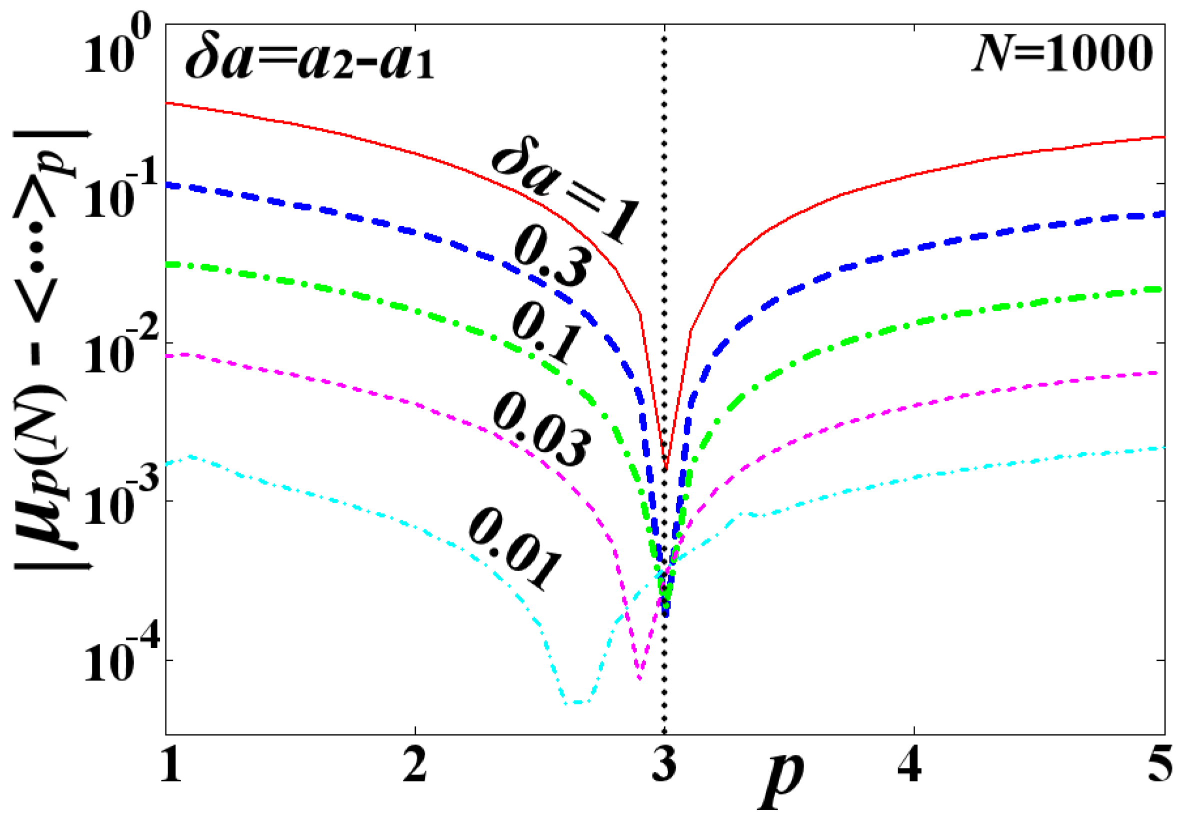
Figure 4 plots the deviation between the -mean estimator and the mean , that is, , and for a large number of data (). The mean is taken for the norm , while the deviation is plotted as a function of the norm p of the estimator. We observe that the deviation is minimized, tending to zero, when the norm is . However, this result holds if the distribution is not symmetric. Once the parameter decreases approaching zero, the distribution becomes symmetric and the deviation obtains small values (while its minimization at a certain p loses its meaning). We observe that for or smaller, the deviation is small enough—of the order of (it is non-zero because of the computation errors caused by the finite N), so that .
5. Conclusions
The Euclidean means are derived by minimizing the sum of the total square deviations, i.e., the Euclidean variance. In a similar way, the non-Euclidean means were developed by minimizing the sum of the deviations, that is proportional to the variance [3]. The main advantage of the new statistical approach is that the p-norm is a free parameter, thus both the -normed expectation values and their variance are flexible to analyze new phenomena that cannot be described under the notions of classical statistics based on Euclidean norms. The least square method based on the Euclidean norm, , and the least absolute deviations method based on the “Taxicab” norm, , are some cases of the general fitting methods based on the -norms (e.g., [15]; for more applications on the fitting methods based on Lp norms, see: [2,4,16,17]; several other applications can be in signal processing optimization and block entropy analysis, e.g., [2]; in image processing, e.g., [18]; in general data analysis, e.g., [5]; in statistical mechanics, e.g., [3,8,19]. The Law of Large Numbers is a theorem that guarantees the stability of long-term averages of random events, but is valid only for metrics induced by the Euclidean norm. The importance of this paper is in extending this theorem for -norms. Other interesting applications will be to establish a central limit theorem applied for the -means.
Acknowledgments
The work was supported in part by the project NNX17AB74G of NASA’s HGI Program.
Conflicts of Interest
The author declare no conflict of interest.
References
- Livadiotis, G. Approach to general methods for fitting and their sensitivity. Physica A 2007, 375, 518–536. [Google Scholar] [CrossRef]
- Livadiotis, G. Approach to the block entropy modeling and optimization. Physica A 2008, 387, 2471–2494. [Google Scholar] [CrossRef]
- Livadiotis, G. Expectation value and variance based on norms. Entropy 2012, 14, 2375–2396. [Google Scholar] [CrossRef]
- Livadiotis, G.; Moussas, X. The sunspot as an autonomous dynamical system: A model for the growth and decay phases of sunspots. J. Stat. Distrib. Appl. 2014, 379, 436–458. [Google Scholar] [CrossRef]
- Livadiotis, G. Chi-p distribution: Characterization of the goodness of the fitting using norms. Physica A 2007, 1, 4. [Google Scholar] [CrossRef]
- Huber, P. Robust Statistics; John Wiley Sons: New York, NY, USA, 1981. [Google Scholar]
- Fréchet, M. Les éléments aléatoires de nature quelconque dans un espace distancié. Ann. L’Institut Henri Poincaré 1948, 10, 215–310. (In French) [Google Scholar]
- Livadiotis, G. Non-Euclidean-Normed Statistical Mechanics. Physica A 2016, 445, 240–255. [Google Scholar] [CrossRef]
- Scarpello, G.M.; Ritelli, D.E. A historical outline of the theorem of implicit functions. Divulg. Mat. 2002, 10, 171–180. [Google Scholar]
- Ahmad, R. On the Structure and Application of Restricted Exchangeability. In Exchangeability in Probability and Statistics; Koch, G., Spizzichino, F., Eds.; Elsevier: Amsterdam, The Netherlands, 1982; pp. 157–164. [Google Scholar]
- Williams, L.R.; Wells, J.H. inequalities. J. Math. Anal. Appl. 1978, 64, 518. [Google Scholar] [CrossRef]
- Feller, W. Law of Large Numbers for Identically Distributed Variables; Wiley: New York, NY, USA, 1971. [Google Scholar]
- Hu, T.C.; Chang, H.C. Complete convergence and the law of large numbers for arrays of random elements. Nonlinear Anal. 1997, 30, 4257–4266. [Google Scholar] [CrossRef]
- Hoffmann-Jørgensen, J.; Su, K.-L.; Taylor, R.L. The Law of Large Numbers and the Ito-Nisio Theorem for Vector Valued Random Fields. J. Theor. Probab. 1997, 10, 145–183. [Google Scholar] [CrossRef]
- Burden, R.L.; Faires, J.D. Numerical Analysis; PWS Publishing Company: Boston, MA, USA, 1993; pp. 437–438. [Google Scholar]
- Sengupta, A. A rational function approximation of the singular eigenfunction of the monoenergetic neutron transport equation. J. Phys. A 1984, 17, 2743–2758. [Google Scholar] [CrossRef]
- Livadiotis, G.; McComas, D.J. Fitting method based on correlation maximization: Applications in Astrophysics. J. Geophys. Res. 2013, 118, 2863–2875. [Google Scholar] [CrossRef]
- Sharma, M.; Batra, A. Analysis of distance measures in content based image retrieval. Glob. J. Comput. Sci. Technol. G Interdiscip. 2014, 14, 11. [Google Scholar]
- Livadiotis, G. Kappa Distributions: Theory and Applications in Plasmas; Elsevier: Amsterdam, The Netherlands; London, UK; New York, NY, USA, 2017. [Google Scholar]
Figure 1.
Example of -means of a dataset following the Poisson distribution. The relation is plotted for (a) , i.e., (red solid line), (blue dash), (green dash–dot), (purple thick dash), (light-blue thick dash–dot); and (b) , i.e., (red solid line), (blue dash), (green dash–dot), (purple thick dash), (light-blue thick dash–dot).
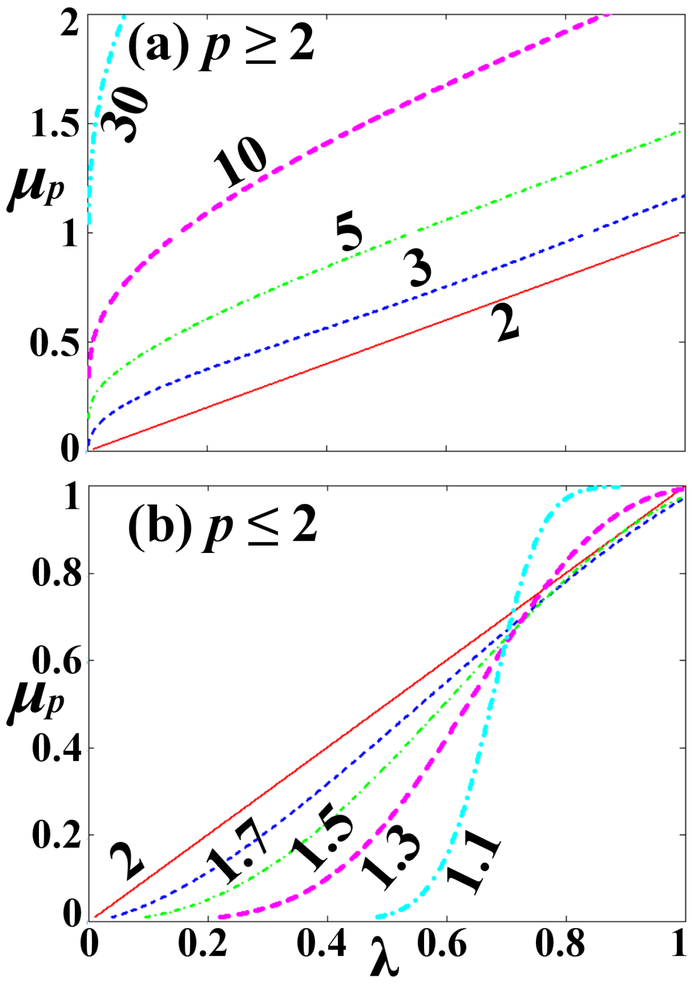
Figure 2.
Uniqueness of the -means of the Poisson distribution. The means are plotted as a function of the p-norm, and for various values of , that is, (red solid), (black dash), and (blue solid).
Figure 2.
Uniqueness of the -means of the Poisson distribution. The means are plotted as a function of the p-norm, and for various values of , that is, (red solid), (black dash), and (blue solid).
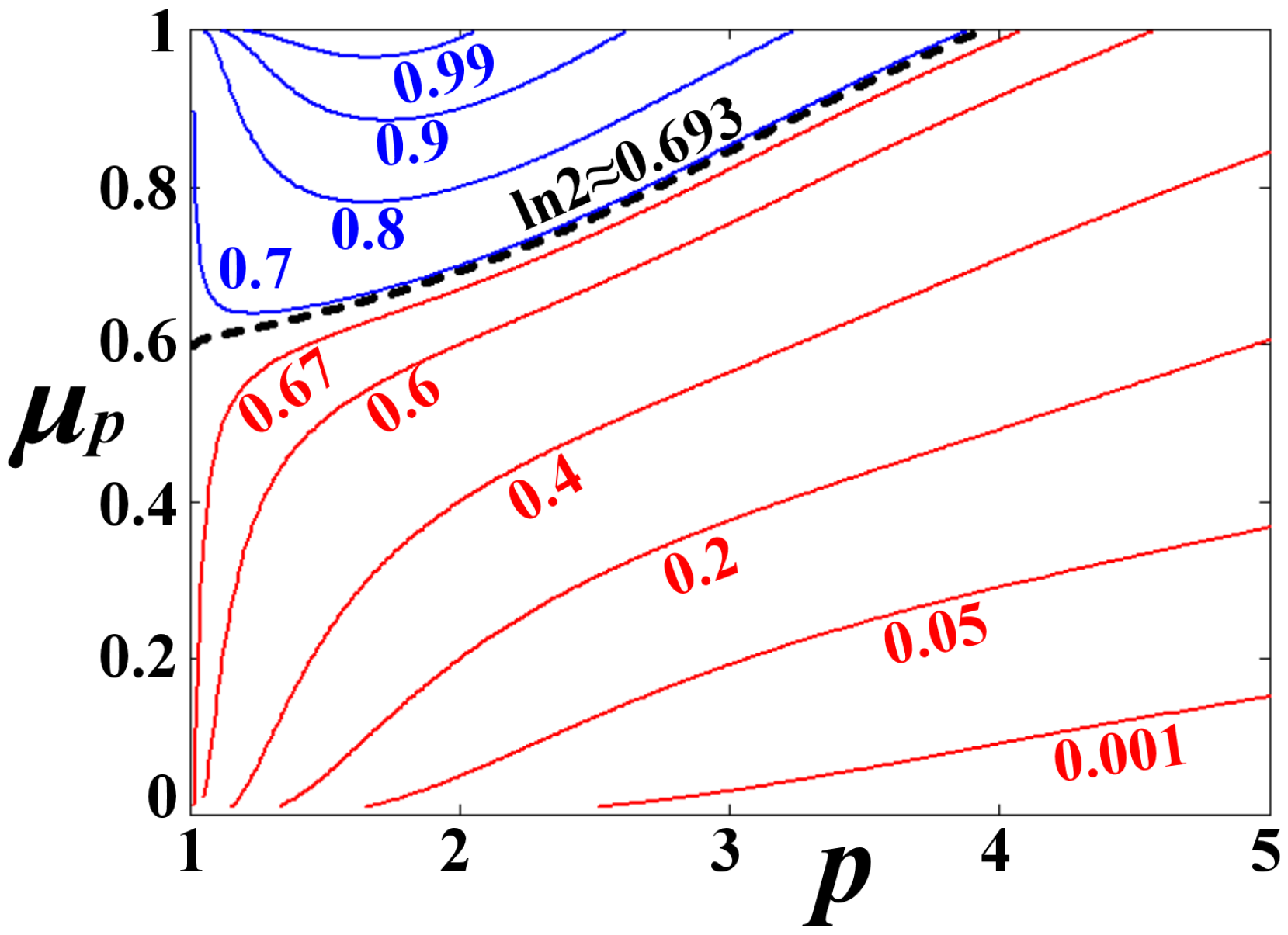
Figure 3.
Convergence of the estimator to the mean (ensemble average). (a) The summation plotted against N for (red solid), 2 (blue dot), and (green dash); (b) The summation plotted against , for (red solid), 2 (blue dot), and (green dash), where holds only for ; (c) Estimator , plotted against the norm p, for and , showing the convergence to the co-plotted mean .
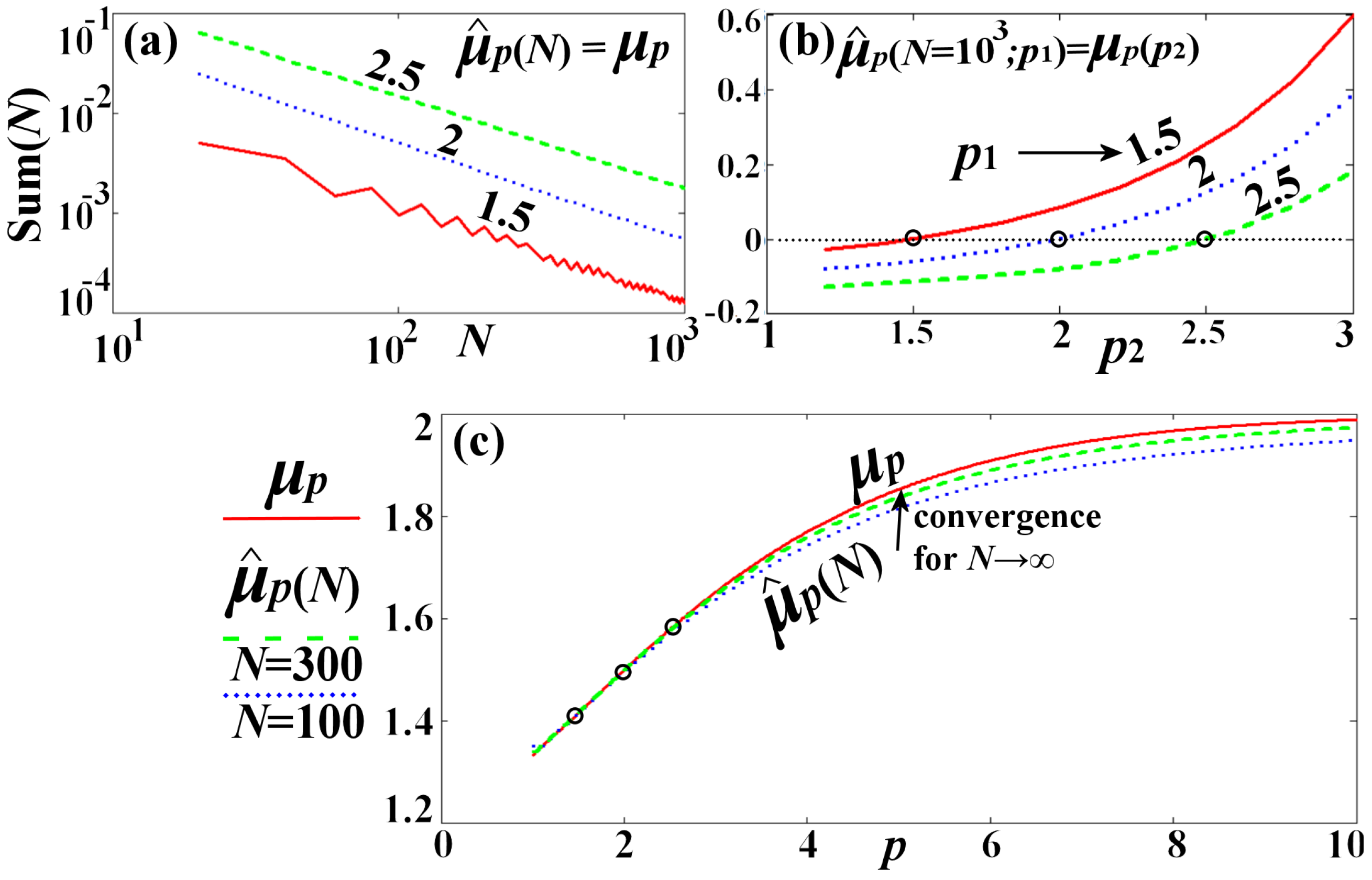
Figure 4.
Deviation is plotted as a function of the p-norm of the estimator, and for various values of the parameter (red solid), (blue thick dash), (green thick dash–dot), (purple dash), and (light-blue dash–dot).
Figure 4.
Deviation is plotted as a function of the p-norm of the estimator, and for various values of the parameter (red solid), (blue thick dash), (green thick dash–dot), (purple dash), and (light-blue dash–dot).
© 2017 by the author. Licensee MDPI, Basel, Switzerland. This article is an open access article distributed under the terms and conditions of the Creative Commons Attribution (CC BY) license (http://creativecommons.org/licenses/by/4.0/).
Share and Cite
MDPI and ACS Style
Livadiotis, G. On the Convergence and Law of Large Numbers for the Non-Euclidean Lp -Means. Entropy 2017, 19, 217. https://doi.org/10.3390/e19050217
AMA Style
Livadiotis G. On the Convergence and Law of Large Numbers for the Non-Euclidean Lp -Means. Entropy. 2017; 19(5):217. https://doi.org/10.3390/e19050217
Chicago/Turabian StyleLivadiotis, George. 2017. "On the Convergence and Law of Large Numbers for the Non-Euclidean Lp -Means" Entropy 19, no. 5: 217. https://doi.org/10.3390/e19050217
Note that from the first issue of 2016, this journal uses article numbers instead of page numbers. See further details here.