
Calculating Iso-Committor Surfaces as Optimal Reaction Coordinates with Milestoning

1
Institute for Computational Engineering and Science, The University of Texas at Austin, Austin, TX 78712, USA
2
Department of Chemistry, The University of Texas at Austin, Austin, TX 78712, USA
*
Author to whom correspondence should be addressed.
Entropy 2017, 19(5), 219; https://doi.org/10.3390/e19050219
Submission received: 17 February 2017
/
Revised: 24 April 2017
/
Accepted: 8 May 2017
/
Published: 11 May 2017
(This article belongs to the Special Issue Understanding Molecular Dynamics via Stochastic Processes)
Abstract
:Reaction coordinates are vital tools for qualitative and quantitative analysis of molecular processes. They provide a simple picture of reaction progress and essential input for calculations of free energies and rates. Iso-committor surfaces are considered the optimal reaction coordinate. We present an algorithm to compute efficiently a sequence of isocommittor surfaces. These surfaces are considered an optimal reaction coordinate. The algorithm analyzes Milestoning results to determine the committor function. It requires only the transition probabilities between the milestones, and not transition times. We discuss the following numerical examples: (i) a transition in the Mueller potential; (ii) a conformational change of a solvated peptide; and (iii) cholesterol aggregation in membranes.
1. Introduction
Determining a reaction coordinate (RC) or an order parameter as a starting point for computational chemistry calculations is a common approach to investigate kinetics. It offers a one-dimensional progress parameter for complex molecular processes in high dimensions. A RC can lead to more efficient computations of rates and simpler interpretations of the simulation results. How to choose an optimal reaction coordinate is a topic of considerable debate. There are two principal uses of a RC that motivate the search for an optimal reaction coordinate.
A RC offers efficient ways to study equilibrium and kinetic observables in complex systems by following the general direction of the coordinate. Methods like umbrella sampling [1], free energy perturbation [2], or blue moon [3] make it possible to calculate free energy profiles along one-dimensional reaction coordinates. Other methods like Transition Interface Sampling [4], Weighted Ensemble [5], Forward Flux [6], and Milestoning [7] allow for computation of rate coefficients or fluxes making use of an order parameter.
A RC allows the projection of the dynamics onto a one-dimensional curve and therefore suggests a simple picture of the mechanism. Examples of methods that provides a one-dimensional view of the reaction progress include the Locally Updated Planes (LUP [8]), Nudged Elastic Band (NEB [9]), and the scalar force [10]. Other approaches are the MaxFlux approach [11,12,13], the String [14], a temperature dependent reaction coordinate [15], and the Dominant Reaction Pathway (DRP [16]). The above approaches provide Minimum Energy Paths, or thermal paths that are locally averaged. They are typically computed in a single step as an optimization of pathways in the whole coordinate space. An alternative approach for computing the desired one-dimensional coordinate is by a two-step operation. The complete space is divided into predetermined “slow” and “fast” variables. Thermal averages are conducted for the fast variables and a minimum free energy path (MFEP) is searched in the effective space of the slow or reduced variables [17].
Both types of reaction coordinates are computed in continuous space, or on a network [13,18,19]. We further comment that the minimum energy path (MEP) and MFEP may encounter the problem of path degeneracy or multiplicity. It is possible, and in complex systems even likely, that more than a single MFEP or MEP connects reactant and products. MFEP, however, is less likely to be degenerate, which makes it better defined and more appropriate for rate calculations. Nevertheless, the predetermined choice of slow variables may miss coordinates that are making significant contribution to the dynamics and rate.
There are two main realizations of a reaction coordinate that connects the states of reactants and products. These views offer theoretical perspective but do not necessarily coincide with the uses mentioned above. The first view is that the reaction coordinate is a curve (a line) that links the reactant and product states. We denote this representation by RL (Reaction Line). The Steepest Descent Path (SDP), which is the line with a minimum energy barrier between the reactant and product states, is an example. Approaches such as LUP [8], scalar force [10], NEB [9], and the zero temperature string [14] compute the SDPs numerically as a set of configurations (points) distributed along the curvilinear coordinate defined in complete space.
The second view of an RC is a progression of non-crossing surfaces from the reactant to the product basins. We denote this second representation by RS (Reaction Surfaces). If the system is of dimension , the RS are of N − 1 dimensions. The RS supplant the line mentioned above and provide a comprehensive picture of the reaction progress. Of course, the two views are not completely separated. Frequently, researchers use a quadratic expansion of the energy landscape in the neighborhood of the RL. The local description defines a plane, which is a model to the RS. The plane is orthogonal to the RL near the point they cross the MEP and at a specific orientation to the line in MFEP. The use of an expansion implicitly assumes that reactive trajectories do not deviate significantly from the line. Moreover, planes cannot be a general solution for non-crossing RS far from the RL if the curve is not strictly linear.
To avoid the problem of hypersurfaces that cross and therefore do not provide a unique reaction coordinate, the use of Voronoi tessellation was proposed [20]. Discrete configurations along the reaction coordinate serve as centers of the Voronoi cells [20]. Voronoi tessellation maps the whole space to cells that do not overlap. However, avoiding planes that cross comes at a price. The reactive space, when represented by Voronoi tessellation, can no longer be presented by a one-dimensional reaction coordinate. The focus of the present manuscript, the iso-committors, are non-crossing surfaces between the reactant and product states, forming a set of objects along a one dimensional coordinate, and are suitable for monitoring the progress of the reaction.
In the next section, we define the committor and the iso-committor surfaces. These functions are computationally expensive and in practice approximations are used to estimate their value. We follow the discussion about the committor by a brief introduction of the method of Milestoning. We then show that the Milestoning algorithm allows for efficient calculations of iso-committor surfaces. The iso-committor surfaces we compute, go beyond the plane assumption [17] or a linear combination of selected coarse variables [21]. As a result, the new presentation is likely to provide new insight into complex reaction events.
2. Materials and Methods
2.1. The Committor
Consider a system of two metastable states and denoting reactants and products respectively. Trajectories are computed, starting from any phase space point and are terminated when they reach either R or P. The committor, , is the probability that a pathway initiated at will make it to the product state (P) before the reactant state (R). The committor is zero at R and one at P, and its range is . The iso-committor surfaces are the set of all phase space points such that the committor function of these points is a constant. It forms a foliation that is useful for the definition of the reaction coordinate. The calculation of the committor function attracted considerable attention. Pioneering work on committors was done in the context of Transition Path Theory (TPT [18,22,23,24]). Indeed the algorithm proposed in the present work is similar to these previous studies. It is also similar in spirit to references [25,26]. However, there are conceptual and algorithmic differences between these investigations, which are discussed later in the article.
For overdamped Langevin dynamics, a partial differential equation (PDE) determines the iso-committor surfaces [27]. The solution of the PDE is rapid and efficient. However, it is limited to a small number of degrees of freedom since the complexity of the solution increases exponentially with the dimensionality of the system. Studies of committors [26,28,29,30] in systems with high dimension use estimates based on trajectory sampling. Trajectory-based formulation makes it possible to use arbitrary dynamics and not limit the choice to overdamped Langevin. Nevertheless, even with trajectory-based approaches calculating exact iso-committor surfaces is computationally challenging. To exhaustively compute the committor function an ensemble of stochastic trajectories is required for each phase space point between R and P.
Given the staggering costs of computing the exact committor surfaces, it is not a surprise that approximate approaches to determine this function are used. Among these approaches are the use of planes in a specific orientation with respect to the SDP curve [17], maximum likelihood determination of function parameters [29], and more [25,28]. In these approaches several different approximations were used: (i) the committor is assumed to depend only on a small number of coarse variables; (ii) Some techniques use only a small displacement from the mean curve; (iii) The committor is assumed to be a linear function of several coordinates. The assumptions mentioned above leave room for improvements, or for the use of alternative approaches to supplant current methodologies.
In the present manuscript, we suggest an alternative calculation of the committor function using Milestoning with several coarse variables [31,32,33]. Milestoning is a theory and an algorithm that computes efficiently the kinetics and thermodynamics of a system using short-time trajectories between boundaries of cells or milestones. In the next section, we briefly review the critical elements of Milestoning and refer the interested reader to other papers [7,31,32,33] for a complete description.
2.2. Milestoning
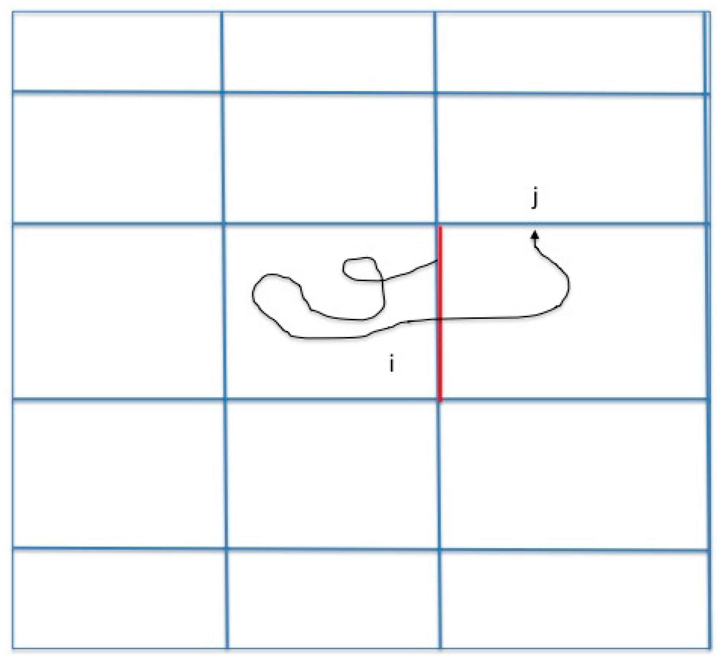
We consider a system with two metastable states, a reactant state R and a product state P. A coordinate vector represents a single configuration and denotes a trajectory as a function of time . The dynamics that we consider are classical but otherwise left for the user to choose. We are interested in conversions of reactants to products and Milestoning is a technique to sample these transitions efficiently. In the past we showed how Milestoning can be used to determine pathways of maximum flux [13]. Here we study another reaction coordinate (the committor). A brief review of Milestoning therefore follows. In Milestoning we consider only short trajectories between boundaries of cells that are called milestones (Figure 1).
A critical operator of the Milestoning theory is the matrix , which is the probability that trajectories initiated at milestone will reach milestone before any other milestone. It is also called the kernel. The transition matrix is time independent and is especially useful for a stationary process. It is obtained from the time-dependent transition probability, (the probability density of a transition between and per unit time at time ). We integrate to obtain . Note that the matrix is normalized with respect to the final state and it may represent a non-Markovian process. For the process to be Markovian the transition probability per unit time must be of the form , i.e., decaying exponentially in the time [7]. The average lifetime of a trajectory initiated at milestone until it hits for the first time another milestone is . The kernel is computed numerically from the trajectories (see below) and it frequently deviates from the Markovian form.
The kinetic of the complete process is determined by the distribution of the first passage times from reactants to products. The complete distribution is hard to determine computationally, and typically only the first moment or the mean first passage time is reported. Milestoning, however, makes it possible to determine all the moments of the distribution from local information. The local information is the moments of the milestones’ life times, or the time moments of . Given this information, explicit expressions for the moments of the first passage time are derived (see [33]). For example, a local moment that we need can be . Another example is . A Markovian model agrees with the general process only in the zero and first time moments [33], which may be a problem if higher time moments are needed. For the calculation of the committor function only the zero moment is necessary, making it possible to use Markovian modeling, with the Markov model properly defined. As discussed earlier must decays exponentially in time with relaxation time of .
To use Milestoning the following two conditions must be met. First, the milestones must be able to differentiate between reactants and products, i.e., there is a subset of milestones that bounds the reactants and another subset of milestones that bound the products and the two sets have zero overlap. Second, there is a sequence of transitions between milestones connecting the reactant and product with non-zero probability. In other words we require that the Mean First Passage Time (MFPT) between the reactant and the product is finite.
A fundamental Milestoning equation determines the stationary flux (the number of trajectories that pass milestone per unit time under stationary conditions) [31,33].
We use bold-faced symbols to denote vectors and matrices. The length of the vector is the number of milestones , and the dimensionality of is . The origin of this equation is the time dependent formulation of Milestoning discussed at length elsewhere [31]:
where is the distribution at zero time (initial conditions). Note that the time range is between 0 and infinite. Integration over time for the delta function in the first term on the right gives one half since the Dirac’s delta function is symmetric. The above equation is a general statement of conservation of trajectories in time. A trajectory that passes a milestone at time and is counted for in the flux vector must originate from other milestones at an earlier time (counted in the flux vector ) and propagate to the milestone of observation after time with a probability determined by the kernel . The process is homogeneous in time and therefore the kernel depends only on the time difference.
If we consider the limit of long time of the time dependent equation and use Laplace transforms we obtain Equation (1) [31]. We can understand this result, however, on a more physical ground. At stationary conditions the flux that passes at each milestone is a time-independent constant, per definition. We therefore have . Moreover, we always set the kernel to have a short range in time. In molecular simulations it decays to zero in sub-nanosecond timescales in most practical applications. Consider the convolution on the right hand side. If is large, so must be to ensure non-zero values of the kernel as a function of the time difference . So we must also have and approaching infinity to avoid approaching zero. As a result we have which is a time independent flux that can be taken out from the convolution integral. Finally the remaining integral becomes . Summarizing the above considerations we obtain from the long time limit of the time-dependent equation, which is Equation (1).
According to Equation (1) the stationary flux is the left eigenvector of the kernel with an eigenvalue one. The matrix is a probability matrix for stochastic transitions between pairs of milestones. The elements of the matrix are all non-negative and the summation of the entries of any row is one. For this matrix the absolute magnitudes of the eigenvalues are equal or smaller than one.
In the exact variant of Milestoning [33], the kernel is a function of the phase space positions in the initiating and terminating milestones. That is where is a phase space point in milestone . The exact kernel is a high dimensional operator which makes its direct use challenging. A systematic simplification is desired and discussed below. We can write the flux through milestone without loss of generality, as a product.
where is a scalar which is the overall weight of a milestone and is the normalized probability density at milestone (). We can redefine the kernel after averaging over the positions in the milestone and summing over the final state.
Equation (3) is then plugged in Equation (1) to provide an equation for the milestone weights—:
The lower formula in Equation (4) is easy to solve since the number of milestones and not the distribution within the milestone determines the dimensionality of the matrix. The complication using Equation (4) is that, in general, is not known. In exact Milestoning we determine progressively more accurate approximations to and to the flux using iterations of Equation (1) [33]
The superscript denotes the iteration number. For example, is our first approximation to the flux at milestone . We choose and we sample configurations in the milestone according to the canonical distribution. With initial distributions at hand, we compute the short trajectories between the milestones and estimate the elements of the matrix according to Equation (3). We continue to determine the weights of the milestones (Equation (4)) and the fluxes . The exact version of Milestoning uses the newly generated distribution of terminating trajectories at the milestones to define and re-computes the weight of the next iteration, repeating the calculations until the process converges. The process is assumed converged if the fluxes remain constant, or an observable of interest, such as the MFPT, does not change its value significantly from iteration to iteration. In the simpler version of Milestoning [7] we stop after determining assuming that the Boltzmann distribution is adequate. Rapid convergence of averages with respect to the distribution is expected for systems at, or close to equilibrium. We tested the use of a single iteration for the system of solvated alanine dipeptide [34] and numerous other applications.
In the present manuscript, we use Milestoning with a single iteration. However, the procedure described here is directly applicable also for exact Milestoning [33]. We estimate the transition kernel from trajectories as:
where is the total number of times a trajectory crossed (or was initiated at) milestone and is the number of trajectories that cross milestone after they passed (or initiated at) milestone . Note that to normalize we must have .
Instead of running many short trajectories between milestones it is also possible to use Milestoning as an analysis tool and to extract the necessary transitions from a long trajectory. A long trajectory, with many reactive events at equilibrium is an exact representation of the dynamics and it can be used to study the committor function and the time scales of the reaction. Hence, the distribution extracted from the long trajectory is exact (the accuracy is restricted only by statistics). We simply monitor the long trajectory and record the milestones that it crosses and the position of the trajectory in the milestone at the crossing to determine the desired distribution function. With the exact results for the distribution at hand, there is no need for the iterations described in Equation (5). We can answer the question “Given that milestone was crossed, what is the probability that the next milestone to be crossed is ?” exactly. The answer to that question, which can be estimated numerically from the data collected from the long trajectory, is the matrix element .
When the milestones are iso-committors or so-called optimal milestones [27], they are (of course) assigned constant probability to reach the product before the reactant and as a result the kernel in Equation (1) is also an independent of the coordinates in the milestone. The collection of the milestones with the same committor value defines an iso-committor surface. The optimality of the committor hyper-surfaces adds another motivation to the present manuscript. The iso-committor surfaces that we determine with the approach discussed in the next section can be used to redefine the milestones and conduct a new analysis of the long trajectory results with optimal milestones.
2.3. The Committor Function and Milestoning
The theory and algorithm that we propose below follow closely the mathematical approach described in reference [35]. On the physics side, our algorithm is similar to the Transition Path Theory of E and Vanden Eijnden, which made the committor a core function of their theory [22,24], and to the explicit formulation of Cameron and Vanden-Eijnden [18]. Our results are analogous to Equation (6) of [18]. However, their core operator, , is an infinitesimal Markovian propagator in time, our is , which describes also non-Markovian and stationary (time-independent) flux [7].
The current formulation uses only a single function that is readily available in Milestoning simulations: the kernel. The kernel, , provides transition probabilities between nearby milestones and is estimated from short trajectories or trajectory fragments between the milestones. It is time independent and is equally applicable to systems in equilibrium or not (if an appropriate function can be found for a non-equilibrium process).
In the Milestoning context, we define the committor function as “Given that we start a trajectory at milestone what is the probability that it will make it to one of the milestones surrounding the product state before the milestones that surround the reactant”? In contrast, we define the kernel as a local function that provides transition probabilities between nearby milestones without crossing other milestones during the transition. In this section, we outline two approaches to determine the committor from the kernel.
The committor is assumed constant in milestone and is defined as the probability of making it from to the product before reaching the reactant for the first time. We denote all the milestones that emerge from the reactants by and all the milestones that lead to the product by . We adjust the kernel such that all probabilities for all i exiting the reactants are zero. We also set . The last choice implies that . Hence, all the trajectories that make it to the product get “stuck” in the product state. Starting from a milestone there may not be a non-zero element and therefore the product state cannot be reached in a single “step”. Multiple “steps” are necessary, and depending on the values of the kernel, the number of steps can be large, as illustrated in the example below. To distinguish the adjusted transition probability from the usual kernel of Milestoning we denote the new definition by . A simple example below illustrates the new construction. Consider a system with four milestones, one that leads to the reactants, one that leads to products, and two intermediate states. Once the flux makes it to the reactant it vanishes. Once the flux reaches the product, it stays in the product with probability one. The is therefore:
First, we consider the calculation of the flux by power iteration . Let us assume that the initial flux is . After one multiplication by the transition matrix, we obtain a vector . After 10 iterations converged (with error smaller than 10−3) to . The elements of the stationary vector are all zero excluding the product entry.
The committor function is obtained by similar power iterations of the matrix on the right side.
Interestingly the matrix converged after only 4 iterations (with errors less than 10−3) to:
Equation (7) is also an iterative adjustment of a vector, consider:
Equation (8) defines iterations of matrix-vector multiplications that converge to the same desired result as Equation (7) in the limit of . For high powers of the transition matrix , the resulting matrix is guaranteed to converge to a fixed value since the absolute magnitudes of the eigenvalues of this matrix are less or equal one. As we multiply the matrix by itself all of its elements are approaching zero excluding the column of the product state (i.e., only for ). These matrix entries are the probabilities that a trajectory that starts at milestone will terminate at the product state and not at the reactant in, at most, steps. Hence, these elements are the values of the committor function of milestone . When multiple milestones bound the product, the value of the committor is a sum over the entries leading to the product. .
We can use Equation (8) as a base for an iterative algorithm to determine . We multiply the current estimate for the committor vector, by and check if the resulting vector converged to the asymptotic value. A convergence check is provided by where is the error tolerance.
The dimensionality of the matrix is the number of milestones, , which is of order of 100 to 10,000. Multiplying a matrix by a vector requires operations if the matrix is dense. The multiplication requires only the non-zero elements of the matrix (in our case about operations) if the matrix is sparse. However, the multiplications are repeated many times and can be computationally expensive. The iteration will converge more rapidly if the eigenvalue gap is significant. In other words, that the difference between the largest and the rest of the eigenvalues is big.
The second algorithm to determine the committors from a Milestoning kernel is based on solving linear equations. The advantage of the linear formulation is that many algorithms are available to address this type of linear problems. Consider trajectories that start at milestone . The committor value of milestone is . In a single transition, the trajectories cross milestones with probabilities for all . The sum is set to one, and therefore all the trajectories that start at are accounted for. The committor values of all the trajectories after the first step is the sum of the probabilities that they made it to milestone multiplied by their committor values : . This probability must be equal to the initial value of the committor . We have:
If we insert the boundary conditions and to the equation we have for all
We can write more compactly Equation (10) as
Equation (11) is a straightforward linear equation for the committor coefficients that is solved by standard approaches. Note that because of the boundary conditions for at the reactant and the product the equation is not homogeneous and has a unique solution.
The solution of Equation (11) is the same as the solution of Equation (8). We show that by substituting in (11) the solution from Equation (8)
The last equality is a result of the convergence of the power iterations, which proves that the solution of Equation (8) solves Equation (11). Since the solution is unique we demonstrate the equivalence of the two approaches.
For an illustration, we are using a long time trajectory to determine the kernel in the examples provided in this manuscript. The long path is decomposed to trajectory fragments between milestones to obtain transition statistics. Instead of a long trajectory, it is possible to use an ensemble of short trajectories with initial conditions sampled at the milestones [31,33,34]. Use of multiple paths is much more efficient than the calculations of a single trajectory, and motivation for the use of the Milestoning algorithm [34]. Nevertheless, a single long trajectory is trivial to conduct using any Molecular Dynamics software. The sampling of initial conditions and on-the-fly recording of crossing events with short trajectories are more complex to implement and require additional programming. Here we use a single trajectory to illustrate that straightforward MD software (or pre-computed trajectories) can be used as well to determine committors. There is another advantage of using a long trajectory in the context of Milestoning. The calculation of MFPT is exact in the over damped limit of Langevin dynamics if the milestones are iso-committors [27]. It is possible to use the procedure described in this paper to redefine the milestones as iso-committors. In exact Milestoning or variants of Milestoning that use many short trajectories re-definition of the milestones implies calculations of new trajectories. However, if a long trajectory is at hand there is no need to re-compute dynamic pathways; only a new analysis of transition events through the new milestones is required.
3. Results
We provide three examples of calculations of iso-committor “surfaces”. In the discrete case the iso-committor is a set of points, not necessarily a surface. The first example is a “toy” problem, a transition between two metastable states on the Mueller potential [36]. The second example is a conformational change in a peptide. The third illustration is the formation of a contact pair of two cholesterol molecules embedded in a DMPC membrane. The last two examples are of systems with thousands of degrees of freedom. When the system is large it is common to define milestones in the space of several coarse variables that we denote by the vector . The coarse variables, e.g., distances or torsion angles, must be chosen such that the reactant and product are separated and uniquely defined. The committor in the space of coarse variables is of course approximate.
A milestone is a surface in the reduced space of coarse variables. The choice of the surfaces is flexible. For example, it can be a boundary between Voronoi cells, as proposed by Vanden Eijnden [20]. For the toy problem of the Mueller potential, the “coarse” variables, , are the two degrees of freedom of the system. In the second example of a conformational transition of a peptide the torsional angles and were used as the two elements of the coarse coordinate vector. In the third example, the formation of a contact pair of cholesterol molecules is examined using two variables: The distance between the center of mass of the cholesterol molecule and their relative orientation while embedded in a DMPC membrane.
In the three examples, we used a long time trajectory and Milestoning analysis to estimate the transition kernel. Once the transition kernel was determined, we proceeded with the calculations of the committor as described in previous sections. To determine events of milestone crossing we use centers of Voronoi cells [20], which we call anchors [31]. The configuration belongs to the cell of anchor if the distance between and is shorter than the distances to any other anchor . A transition between cells (or a crossing of a milestone) occurs when the system changes its cell assignment in a single time step. We record crossing events. Correlated events, e.g., crossing milestone i followed by crossing milestone j, are histogrammed. That is, we ask, “What is the probability that crossing milestone will be followed by crossing milestone next?” The answer to this question is and Equation (6).
At most one event of crossing should be detected between sequential time steps. Crossing corners of cells can be interpreted as events of multiple transitions and are a concern. There is a need to use a small time step and frequently save the values of the coarse variables to avoid more than one crossing between two sequential configurations. In the first example, which is a Milestoning calculation on a fine mesh, transitions through corners are detected. We therefore add milestones to account for “corner” transitions.
3.1. Example 1: A Transition between Metastable States on the Mueller Model Potential
In Figure 2 we display the two-dimensional energy landscape of the first example [36,37]. The potential contour lines are in different level of gray (left bar) and the iso-committor values are in colors (right bar). We build a detailed two-dimensional grid in which every edge of a square is a milestone. We did not build a fine mesh at high-energy domains that are unlikely to be visited during the simulations and make a significant contribution to the kinetics. This choice explains the white area that are not covered by fine milestones at the top right and lower left corners. More specifically we consider set of points such that where A is a selected area to avoid very high energy domains. We have and . The length of every edge (a milestone) is 0.05. The total number of milestones is 8,320. The reactant is defined by the milestones surrounding the energy minimum at . The product is at the energy minimum (−0.623, 0.028). We consider dynamics described by overdamped Langevin and equations of motion
where is the time derivative of the two dimensional coordinate vector, is the Mueller potential [37], and the random force was sampled from the normal distribution with a mean of zero and variance of . The friction coefficient was set to one, and the temperature times the Boltzmann constant was set to 10. The equations of motion were integrated for steps for the analysis. Milestoning crossing events were accumulated and were used to determine the matrix K. We used power iterations of the transition matrix to determine the committor. After 3000 iterations we verified convergence by requiring that the sum of row elements that should be exactly zero, is smaller than 0.05, i.e., we require
The iso committor surfaces in Figure 2 show a remarkably simple picture in which the energy barrier (the white curve) is also the surface with iso-committor probability of 0.5. This is the expected behavior of systems with high barriers. However, more complex behavior can be found for systems with more moderate barriers, as we illustrate in the second example.
3.2. Example 2: A Conformational Transition in Alanine Tri-Peptide
Here we consider a transition between metastable states of solvated alanine tri-peptide (Figure 3). The long trajectory of a solvated and blocked tri-alanine (Figure 3) was calculated using version 2.11 of the program NAMD [38] with the CHARMM 36 force field [39].
The trajectory length was 101.86 nanoseconds, and it samples configurations from the NVE ensemble. The box size was and with 608 TIP3P water molecules. The time step was 2 fs. The temperature, measured by the average kinetic energy, was 300 K throughout the simulation. The smooth cutoff distance was , and the pair-list distance was . Short range non-bonded interactions were evaluated each step while long range Lennard-Jones and electrostatic interactions were computed every two step using the RESPA algorithm [40]. The Particle Meshed Ewald method was used with a grid spacing of 1 Å and error tolerance of 10−6.
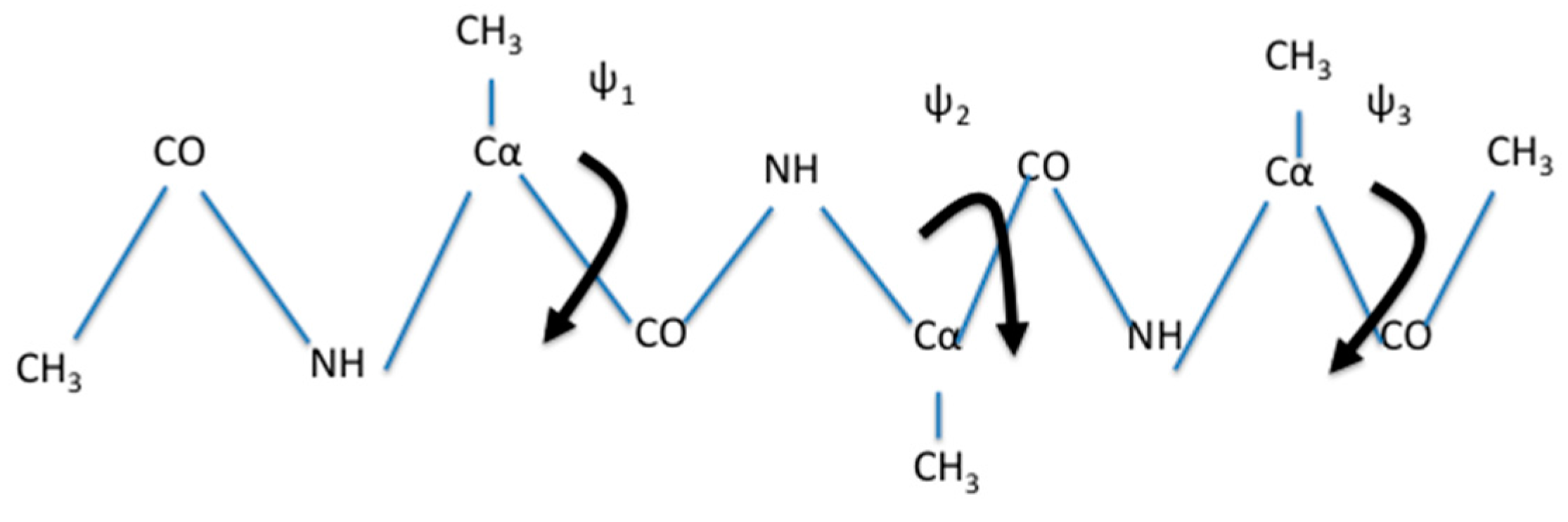
A natural choice for coarse variables to describe backbone transitions in peptide chains are the , and dihedral angles. The torsions of the peptide chain show significantly less flexibility and are not included. We also observed that is locked most of the simulation time in a single minimum (Figure 4). Therefore, we did not choose it as a coarse variable.
For each dihedral angle, we define 12 milestones covering the range between −180 to 180 degrees. The program Miles analyzed the trajectory [41,42]. Miles is available at http://clsb.ices.utexas.edu/web/miles and is a tool that runs and analyzes Milestoning simulations using other MD software packages such as NAMD [38]. Figure 5 shows the canonical probability density of this system as a function of the two dihedral angles and the grid used in the Milestoning calculations. The reactant is the free energy minimum at the top right corner of the figure , and the product is at the lower left . The value of the computed committor is color-coded according to the bar on the right.
The graph makes it possible to visualize a preferred pathway, which is going from the reactants to the product (green line in Figure 5). We can imagine the path as two straight lines. One line starts at the reactants , going in a perpendicular direction upward such that only changes. Then because of the periodic boundary condition it reaches the minimum at the lower right at about from below. Along this line we passed a committor surface of value 0.5 near before we reached an intermediate minimum . From there we follow the horizontal line to the left with fixed at −60 until we reach the minimum of the product at and . The committors in this example were computed using the second algorithm (i.e., solving the linear Equation (11)).
The prediction of the committor values at the milestone is approximate, since the committor is in principle a function of the complete phase space vector and not only of the coarse variables. To test out choice of coarse variables we launch trajectories from milestones with commitment predicted close to 0.5. We sample 100 trajectories for each milestone from the canonical distribution and integrate them in time to termination either at the reactant or the product. The result are summarized in Table 1.
3.3. Example 3: Exchanging Cholesterol Molecules between Aggregates Embedded in Dimyristoylphosphatidylcholine (DMPC) Membrane
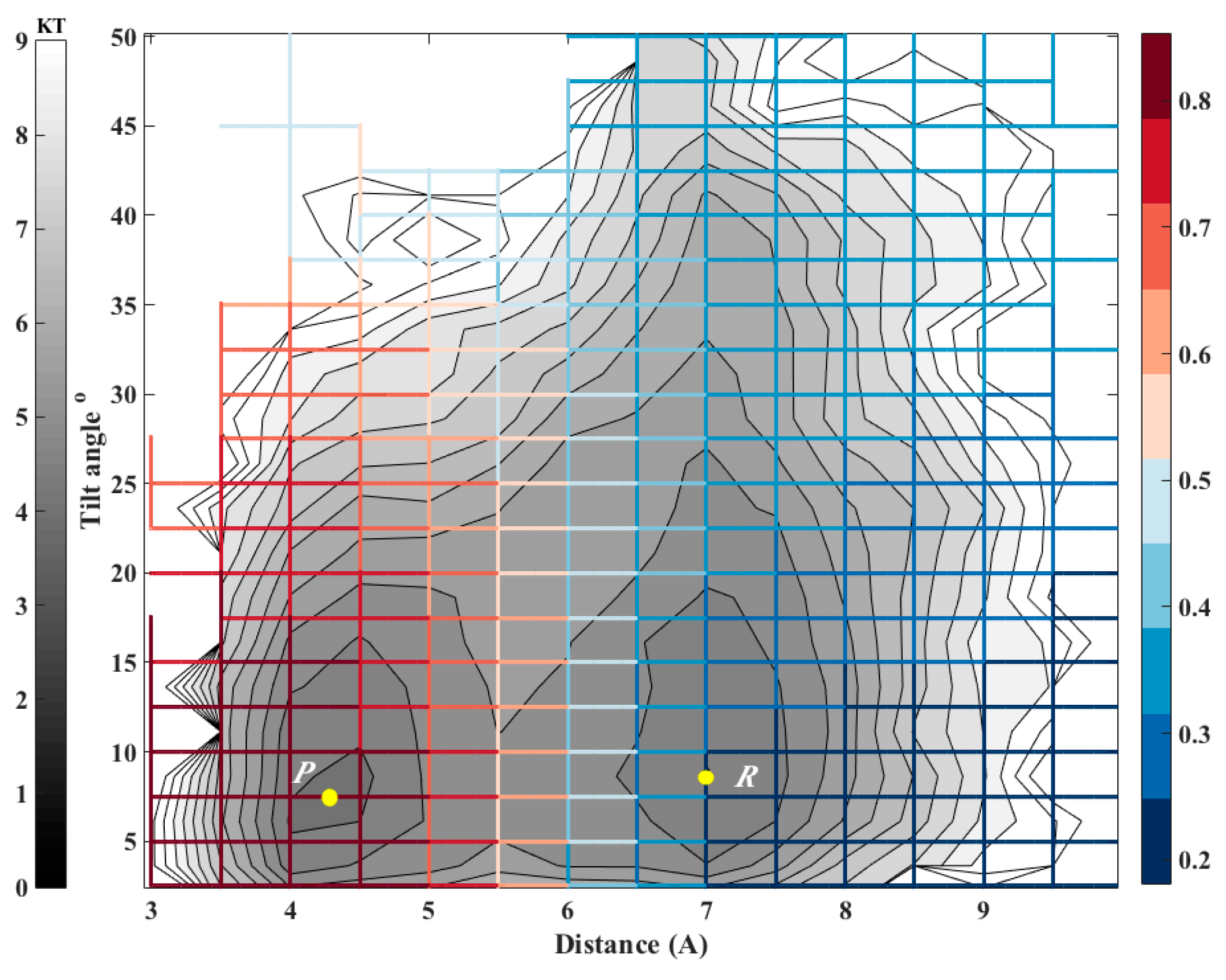
Biological membranes frequently include cholesterols in addition to the phospholipid components. The fraction of these molecules embedded in DMPC membrane may exceed 50 percent by weight. It is therefore of considerable interest to model thermodynamic and kinetic of the heterogeneous membrane-cholesterol environment. Here we consider the transition of a cholesterol molecule between two clusters. An example of this phenomenon is shown in Figure 6 with a top view of the membrane and cholesterol molecules embedded in it. The two clusters of cholesterol molecules are in red and in yellow. During the final 100 ns of simulation, a cholesterol molecule (shown in orange) switches its position from the red cluster to the yellow cluster frequently. To study this transition we examine two coarse variables that may influence contact formation: The distances between the centers of masses of the cholesterol molecules and their relative orientation (Figure 6). At short distances, the orientation of paired cholesterols inclines to be parallel. For this purpose we chose the tilt angle (θ) and the distance between center of masses of the reference cholesterol and the closest cholesterol from the red cluster (r) as our coarse variables. According to Figure 7, the free energy surface shows two minima corresponding to two states where cholesterol 1 is attached to the red or yellow clusters that we define as product and reactant states, respectively. After calculating the committor values for all milestones, it turns out, as we illustrate below (Figure 7), that the orientation of the cholesterol molecules is influenced only weakly by proximity of the two cholesterols and the distance plays a more significant role.
The simulation was conducted in the DMPC membrane with 40 percent cholesterol at 300 K using the MOIL program [44]. There are 48 DMPC and 32 cholesterol molecules in each leaflet. The system was equilibrated for 50 nanoseconds and another 100 ns were used for data collection. Structures were saved every picosecond for further analysis. The trajectory was analyzed to determine events of milestone crossing and to collect statistics to compute the element of the kernel—. The committor function is presented in Figure 7.
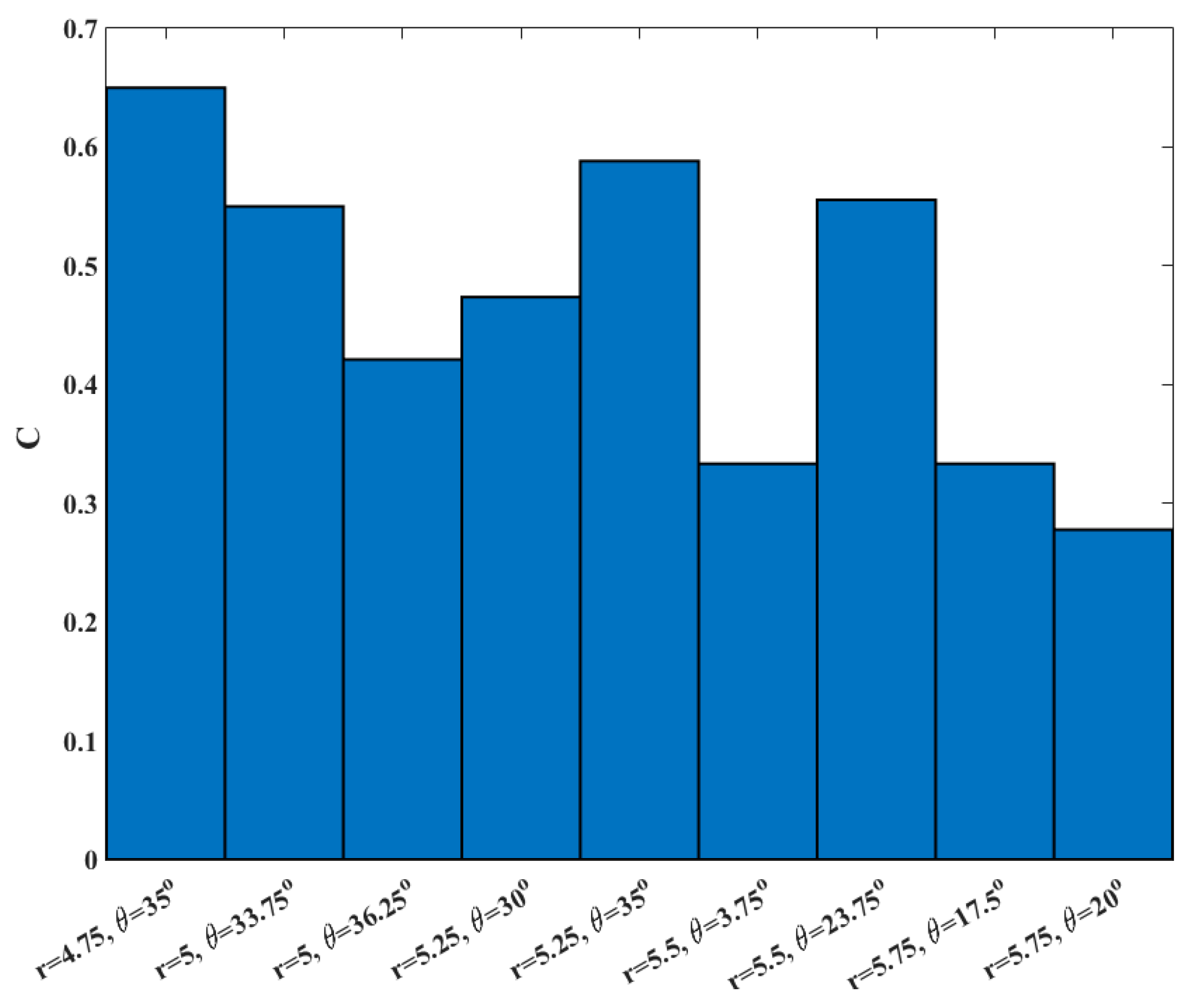
To examine the accuracy of the calculated committor, we considered 9 milestones that have committor values close to 0.5 (0.47 < C < 0.53). Since the systems is large and the simulations are expensive we have a limited statistics for this test. At each milestone we conducted 20 simulations until the trajectories reach the product or the reactant states. Then committor values are estimated by averaging over the results for each milestone. The results are shown in Figure 8.
4. Conclusions
We derived and illustrated a novel algorithm to determine committor functions. The set of iso-committor surfaces with values are considered an optimal reaction coordinate. The algorithm is based on Milestoning calculations [31,33], a technology that exploits the use of short trajectories between cell boundaries to compute overall kinetics and thermodynamics. It is shown that within the resolution of the milestones (boundaries between cells in coarse space), the committor functions are computed efficiently if a long-time trajectory is used in the analysis. The calculations of the kernel can be made more efficient if trajectory fragments are used. By breaking a committor hyper surface to a large number of (small) milestones we can obtain a better approximation to the desired surface than a hyper plane in a specific orientation to the reaction line (RL) which is frequently assumed.
The limitation of the algorithm is the computational costs, which is proportional to the number of active milestones. If the number of coarse variables is large, the number of milestones is likely to be large as well. It is growing exponentially with the number of coarse variables in the worst-case scenario.
Acknowledgments
This research was supported in part by grants from NIH GM059796 and GM111364 and from the Welch foundation F-1896. It was motivated by extensive discussions on the committor function during a weeklong conference in Leiden on “Reaction Coordinates from Molecular Trajectories”.
Author Contributions
Ron Elber developed the basic theory and formulated the power iteration algorithm. Juan M. Bello-Rivas refined the algorithm and formulated the linear equation for the committor. Piao Ma computed the committor function for the Mueller potential, Juan M. Bello-Rivas conducted the simulation and analysis of the peptide. Alfredo E. Cardenas and Arman Fathizadeh performed the simulations and analysis of the membrane system.
Conflicts of Interest
The authors declare no conflict of interest.
References
- Torrie, G.M.; Valleau, J.P. Non-physical sampling distributions in monte-carlo free-energy estimation—Umbrella sampling. J. Comput. Phys. 1977, 23, 187–199. [Google Scholar] [CrossRef]
- Chipot, C. Free Energy Calculations in Biological Systems. How Useful Are They in Practice? Leimkuhler, B., Ed.; Springer: Berlin/Heidelberg, Germany, 2006. [Google Scholar]
- Carter, E.A.; Ciccotti, G.; Hynes, J.T.; Kapral, R. Constrained reaction coordinate dynamics for the simulation of rare events. Chem. Phys. Lett. 1989, 156, 472–477. [Google Scholar] [CrossRef]
- Van Erp, T.S.; Moroni, D.; Bolhuis, P.G. A novel path sampling method for the calculation of rate constants. J. Chem. Phys. 2003, 118, 7762–7774. [Google Scholar] [CrossRef]
- Zhang, B.W.; Jasnow, D.; Zuckerman, D.M. The “weighted ensemble” path sampling method is statistically exact for a broad class of stochastic processes and binning procedures. J. Chem. Phys. 2010, 132. [Google Scholar] [CrossRef] [PubMed]
- Allen, R.J.; Valeriani, C.; ten Wolde, P.R. Forward flux sampling for rare event simulations. J. Phys. Condens. Matter 2009, 21. [Google Scholar] [CrossRef] [PubMed]
- Faradjian, A.K.; Elber, R. Computing time scales from reaction coordinates by milestoning. J. Chem. Phys. 2004, 120, 10880–10889. [Google Scholar] [CrossRef] [PubMed]
- Ulitsky, A.; Elber, R. A new technique to calculate steepest descent paths in flexible polyatomic systems. J. Chem. Phys. 1990, 92, 1510–1511. [Google Scholar] [CrossRef]
- Jonsson, H.; Mills, G.; Jacobsen, K.W. Nudged elastic band method for finding minimum energy paths of transitions. In Classical and Quantum Dynamics in Condensed Phase Simulations; Berne, B.J., Ciccotti, G., Coker, D.F., Eds.; World Scientific: Singapore, 1998; pp. 385–403. [Google Scholar]
- Olender, R.; Elber, R. Yet another look at the steepest descent path. J. Mol. Struct. Theochem 1997, 398–399, 63–71. [Google Scholar] [CrossRef]
- Huo, S.H.; Straub, J.E. The MaxFlux algorithm for calculating variationally optimized reaction paths for conformational transitions in many body systems at finite temperature. J. Chem. Phys. 1997, 107, 5000–5006. [Google Scholar] [CrossRef]
- Berkowitz, M.; Morgan, J.D.; McCammon, J.A.; Northrup, S.H. Diffusion-controlled reactions—A variational formula for the optimum reaction coordinate. J. Chem. Phys. 1983, 79, 5563–5565. [Google Scholar] [CrossRef]
- Viswanath, S.; Kreuzer, S.M.; Cardenas, A.E.; Elber, R. Analyzing milestoning networks for molecular kinetics: Definitions, algorithms, and examples. J. Chem. Phys. 2013, 139. [Google Scholar] [CrossRef] [PubMed]
- E, W.N.; Ren, W.Q.; Vanden-Eijnden, E. String method for the study of rare events. Phys. Rev. B 2002, 66, 4. [Google Scholar] [CrossRef]
- Elber, R.; Shalloway, D. Temperature dependent reaction coordinates. J. Chem. Phys. 2000, 112, 5539–5545. [Google Scholar] [CrossRef]
- Faccioli, P.; Sega, M.; Pederiva, F.; Orland, H. Dominant pathways in protein folding. Phys. Rev. Lett. 2006, 97. [Google Scholar] [CrossRef] [PubMed]
- Maragliano, L.; Fischer, A.; Vanden-Eijnden, E.; Ciccotti, G. String method in collective variables: Minimum free energy paths and isocommittor surfaces. J. Chem. Phys. 2006, 125. [Google Scholar] [CrossRef] [PubMed]
- Cameron, M.; Vanden-Eijnden, E. Flows in Complex Networks: Theory, Algorithms, and Application to Lennard-Jones Cluster Rearrangement. J. Stat. Phys. 2014, 156, 427–454. [Google Scholar] [CrossRef]
- Berezhkovskii, A.; Hummer, G.; Szabo, A. Reactive flux and folding pathways in network models of coarse-grained protein dynamics. J. Chem. Phys. 2009, 130. [Google Scholar] [CrossRef] [PubMed]
- Vanden-Eijnden, E.; Venturoli, M. Markovian milestoning with Voronoi tessellations. J. Chem. Phys. 2009, 130. [Google Scholar] [CrossRef] [PubMed]
- Peters, B.; Trout, B.L. Obtaining reaction coordinates by likelihood maximization. J. Chem. Phys. 2006, 125. [Google Scholar] [CrossRef] [PubMed]
- E, W.N.; Vanden-Eijnden, E. Transition-Path Theory and Path-Finding Algorithms for the Study of Rare Events. Ann. Rev. Phys. Chem. 2010, 61, 391–420. [Google Scholar] [CrossRef] [PubMed]
- Metzner, P.; Schutte, C.; Vanden-Eijnden, E. Transition path theory for markov jump processes. Multiscale Model. Simul. 2009, 7, 1192–1219. [Google Scholar] [CrossRef]
- Vanden Eijnden, E. Computer Simulations in Condensed Matter: From Materials to Chemical Biology. In Transition Path Theory; Ferrario, M., Ciccotti, G., Binder, K., Eds.; Springer: Berlin/Heidelberg, Germany, 2006; Volume 2, pp. 453–494. [Google Scholar]
- Lechner, W.; Rogal, J.; Juraszek, J.; Ensing, B.; Bolhuis, P.G. Nonlinear reaction coordinate analysis in the reweighted path ensemble. J. Chem. Phys. 2010, 133. [Google Scholar] [CrossRef] [PubMed]
- Banushkina, P.V.; Krivov, S.V. Nonparametric variational optimization of reaction coordinates. J. Chem. Phys. 2015, 143. [Google Scholar] [CrossRef] [PubMed]
- Vanden Eijnden, E.; Venturoli, M.; Ciccotti, G.; Elber, R. On the assumption underlying Milestoning. J. Chem. Phys. 2008, 129. [Google Scholar] [CrossRef] [PubMed]
- Ma, A.; Dinner, A.R. Automatic method for identifying reaction coordinates in complex systems. J. Phys. Chem. B 2005, 109, 6769–6779. [Google Scholar] [CrossRef] [PubMed]
- Peters, B.; Beckham, G.T.; Trout, B.L. Extensions to the likelihood maximization approach for finding reaction coordinates. J. Chem. Phys. 2007, 127. [Google Scholar] [CrossRef] [PubMed]
- Bolhuis, P.G.; Dellago, C.; Chandler, D. Reaction coordinates of biomolecular isomerization. Proc. Natl. Acad. Sci. USA 2000, 97, 5877–5882. [Google Scholar] [CrossRef] [PubMed]
- Kirmizialtin, S.; Elber, R. Revisiting and Computing Reaction Coordinates with Directional Milestoning. J. Phys. Chem. A 2011, 115, 6137–6148. [Google Scholar] [CrossRef] [PubMed]
- Majek, P.; Elber, R. Milestoning without a Reaction Coordinate. J. Chem. Theory Comput. 2010, 6, 1805–1817. [Google Scholar] [CrossRef] [PubMed]
- Bello-Rivas, J.M.; Elber, R. Exact milestoning. J. Chem. Phys. 2015, 142. [Google Scholar] [CrossRef] [PubMed]
- West, A.M.A.; Elber, R.; Shalloway, D. Extending molecular dynamics time scales with milestoning: Example of complex kinetics in a solvated peptide. J. Chem. Phys. 2007, 126. [Google Scholar] [CrossRef] [PubMed]
- Lin, L.; Lu, J.; Vanden-Eijnden, E. A Mathematical Theory of Optimal Milestoning (with a Detour via Exact Milestoning). Available online: https://arxiv.org/abs/1609.02511 (accessed on 9 May 2017).
- Muller, K. Reaction paths on multidimensional energy hypersurfaces. Angew. Chem. Int. Ed. Engl. 1980, 19, 1–13. [Google Scholar] [CrossRef]
- Mueller, K.; Brown, L.D. Location of Saddle Points and Mnimum Energy Paths by a Constrained Simplex Optimization Procedure. Theor. Chim. Acta (Berlin) 1979, 53, 75–93. [Google Scholar] [CrossRef]
- Phillips, J.C.; Braun, R.; Wang, W.; Gumbart, J.; Tajkhorshid, E.; Villa, E.; Chipot, C.; Skeel, R.D.; Kalé, L.; Schulten, K. Scalable molecular dynamics with NAMD. J. Comput. Chem. 2005, 26, 1781–1802. [Google Scholar] [CrossRef] [PubMed]
- MacKerell, A.D.; Bashford, D.; Bellott, M.; Dunbrack, R.L.; Evanseck, J.D.; Field, M.J.; Fischer, S.; Gao, J.; Guo, H.; Ha, S.; et al. All-atom empirical potential for molecular modeling and dynamics studies of proteins. J. Phys. Chem. B 1998, 102, 3586–3616. [Google Scholar] [CrossRef] [PubMed]
- Tuckerman, M.; Berne, B.J.; Martyna, G.J. Reversible multiple time scale molecular-dynamics. J. Chem. Phys. 1992, 97, 1990–2001. [Google Scholar] [CrossRef]
- Bello-Rivas, J.M. Iterative Milestoning. Ph.D. Thesis, University of Texas at Austin, Austin, TX, USA, December 2016. Available online: https://repositories.lib.utexas.edu/handle/2152/45791 (accessed on 9 May 2017).
- Bello-Rivas, J.M.; Elber, R. clsb/miles: v0.0.2. Available online: http://doi.org/10.5281/zenodo.573288 (accessed on 9 May 2017).
- Humphrey, W.; Dalke, A.; Schulten, K. VMD: Visual molecular dynamics. J. Mol. Graph. 1996, 14, 33–38. [Google Scholar] [CrossRef]
- Ruymgaart, A.P.; Cardenas, A.E.; Elber, R. MOIL-opt: Energy-Conserving Molecular Dynamics on a GPU/CPU System. J. Chem. Theory Comput. 2011, 7, 3072–3082. [Google Scholar] [CrossRef] [PubMed]
Figure 1.
A schematic drawing of a Milestoning trajectory. We initiate trajectories at milestone according to a known flux distribution function at the interface: . We terminate the trajectories when they hit for the first time a different milestone (). An example of a single trajectory is displayed. The pathway starts from the red milestone and terminates at a divider . From multiple trajectories we estimate the matrix , which is the probability that a path initiated at milestone will terminate at milestone , where is the number of trajectories initiated at milestone and the number of trajectories initiated at that terminated at . Note that .

Figure 2.
The iso-committor surfaces for the Mueller potential computed for overdamped Langevin dynamics. See text for more details.
Figure 2.
The iso-committor surfaces for the Mueller potential computed for overdamped Langevin dynamics. See text for more details.
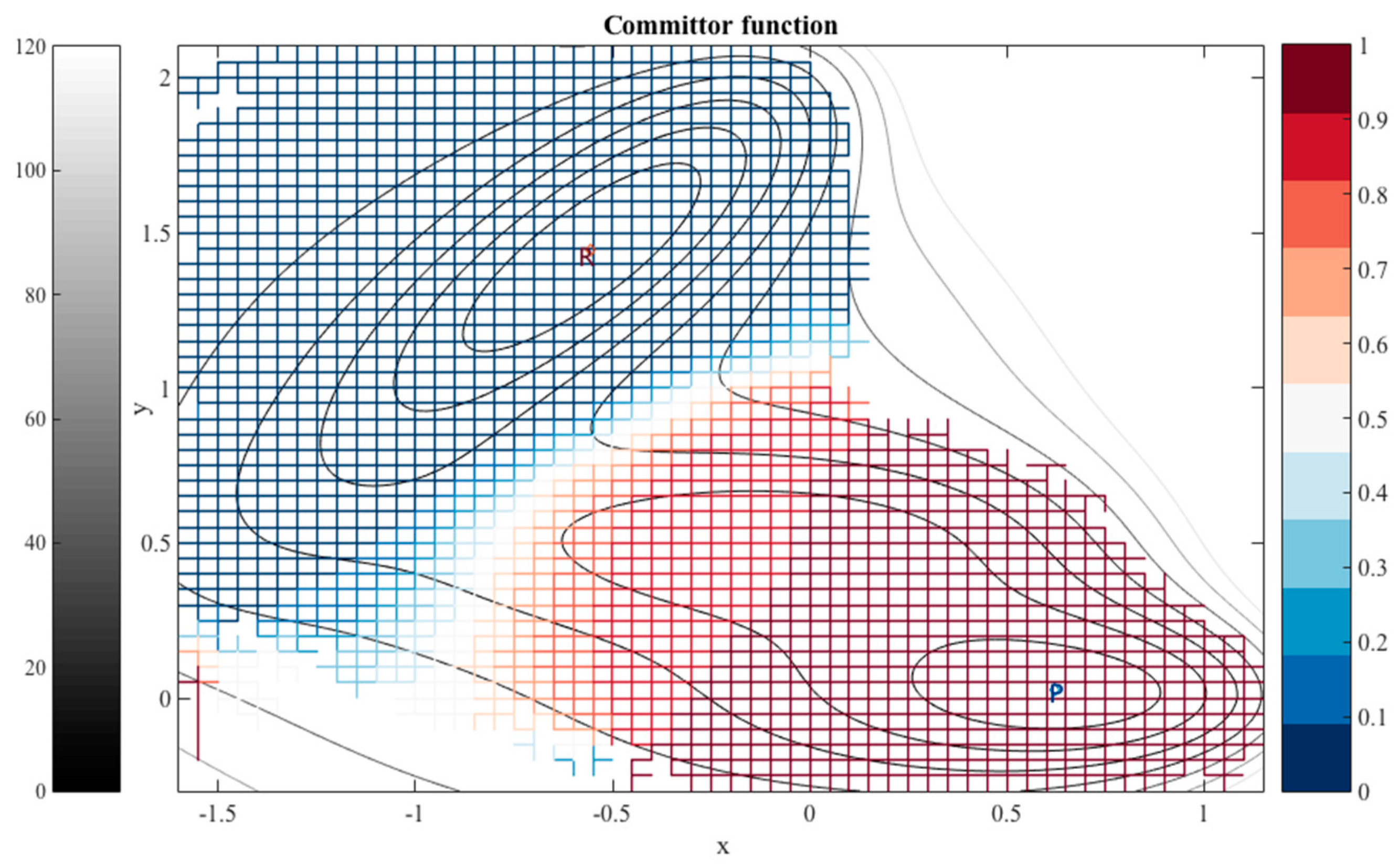
Figure 3.
A schematic drawing of a blocked trialanine. We also show the three dihedral angles that are considered for the coarse variables: and . They are shown as rotations around bonds. In the simulations it turns out that has a restricted distribution (see also Figure 4) and therefore was not considered as a coarse variable in the calculation described below.

Figure 4.
The probability density of the dihedral angle of alanine tripeptide. The values of the torsion were extracted from a trajectory and binned. The distribution consists of a single maximum near 160 degrees, and another metastable state near 50 degrees, which is barely populated.
Figure 4.
The probability density of the dihedral angle of alanine tripeptide. The values of the torsion were extracted from a trajectory and binned. The distribution consists of a single maximum near 160 degrees, and another metastable state near 50 degrees, which is barely populated.
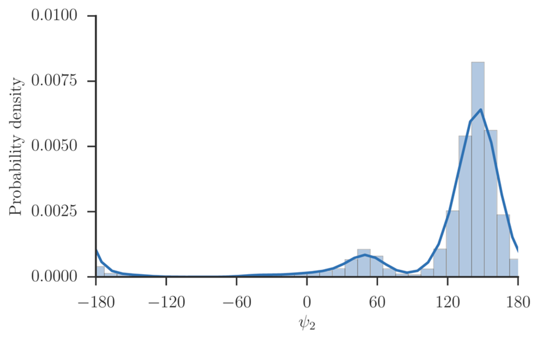
Figure 5.
The committor function, colored-coded according to the bar on the right, is determined on a square grid and shown on the canonical probability density of two coarse variables of tri-alanine. The green arrowed line is a schematic reaction coordinate to guide the eye. It starts at the reactant and follows a steepest descent direction in committor space to the product. The iso-committor surfaces are determined in the space of coarse variables and are therefore approximate. See text for more details.
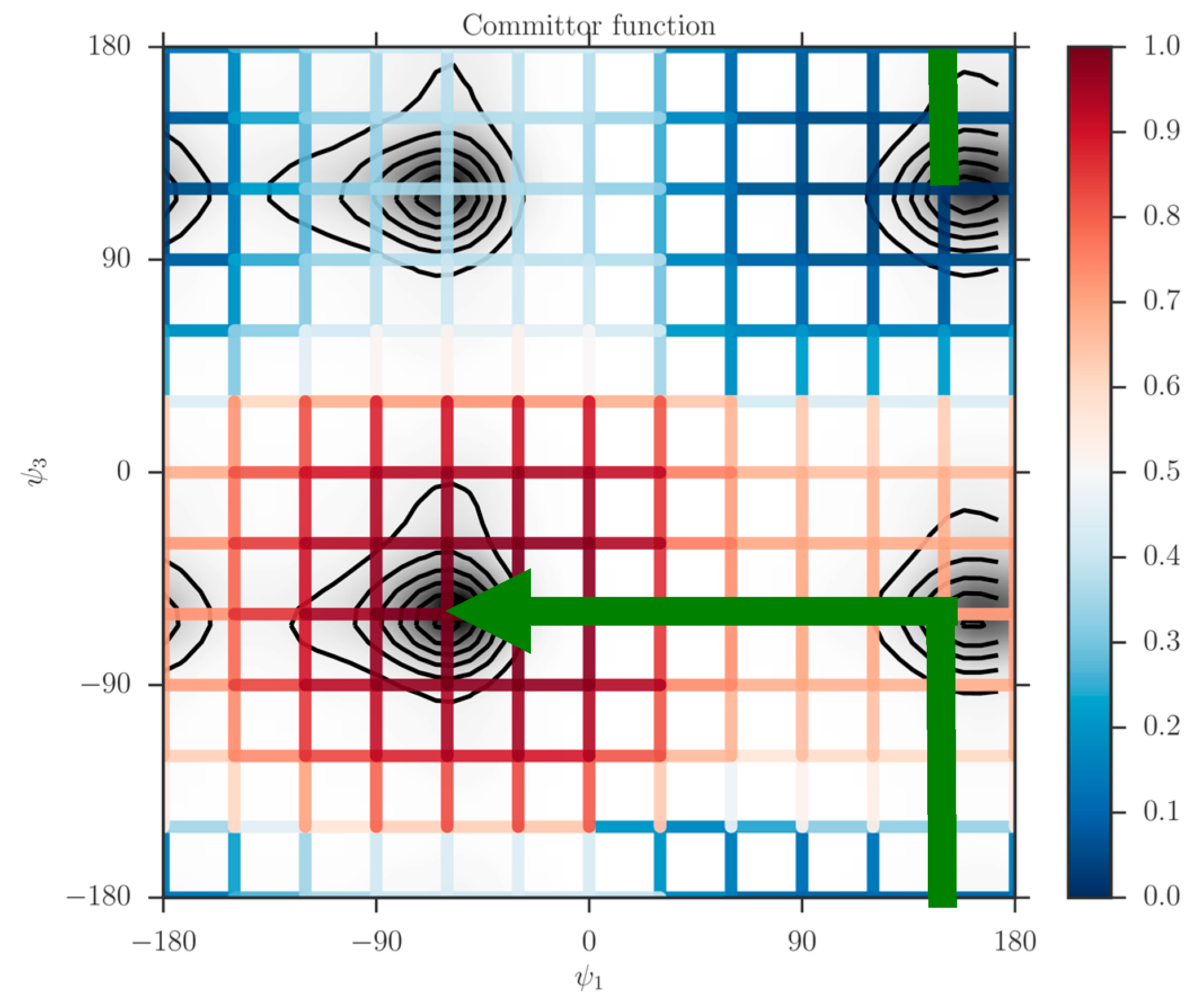
Figure 6.
(Left): A top view of the membrane box. Cholesterol molecules are illustrated with colored spheres and the DMPC molecules are shown with gray lines. The two cholesterol clusters of interest are shown in red and yellow with an orange cholesterol molecule transitions between the two clusters. (Right): A schematic representation of the coarse variables that determine the relative position of two cholesterol molecules 1 and 2. The dashed line shows the distance between their centers of mass and the green solid arrows represent the tilt vector for each cholesterol molecule. The tilt vectors are unit vectors along the line connecting atoms C3 and C17 of the cholesterol molecule. The tilt angle is defined as the angle between the tilt vectors. The plot was prepared with the VMD program [43].
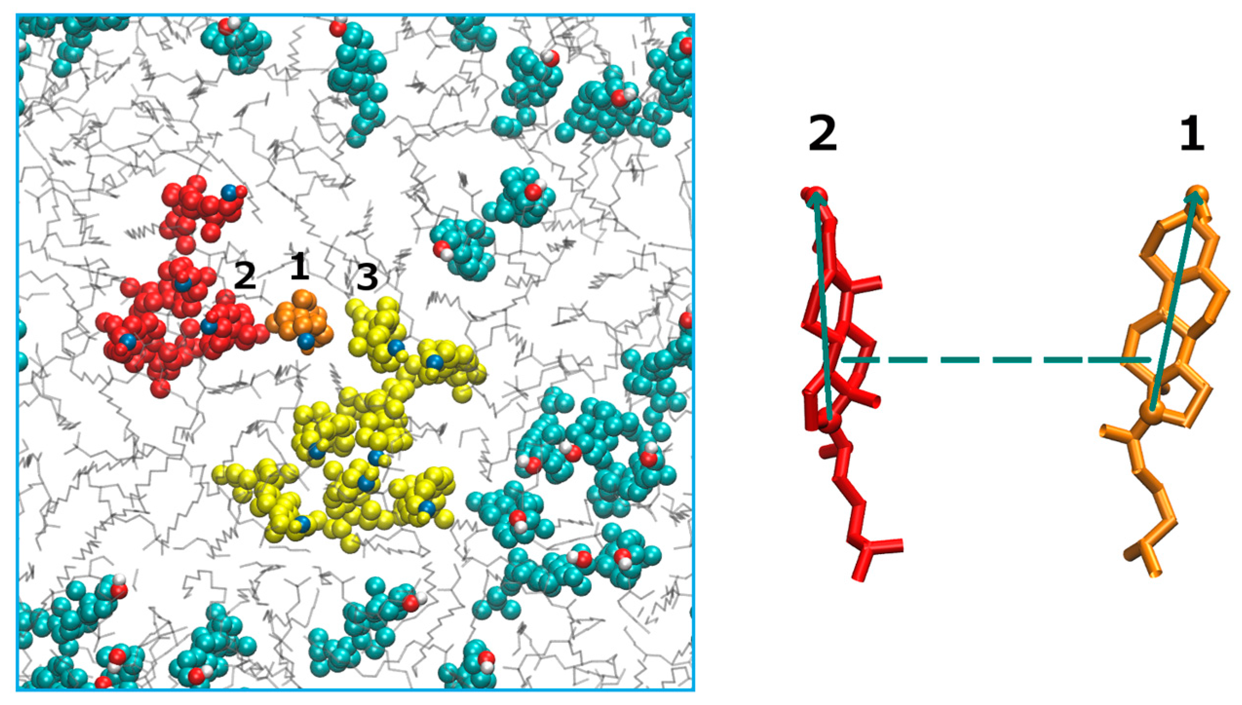
Figure 7.
The committor function for exchanging a molecule between two adjacent clusters of cholesterol molecules embedded in a DMPC membrane. The iso-committors are shown as a function of the distance between the centers of masses of the molecules and their relative tilting angle. The gray lines are equipotential curves of the free energy landscape. The committor function (color coded) was computed on the grid by solving the linear equation (second algorithm, Equation (11)). Note that the committor function depends primarily on the distance and less on the orientation. The iso-committor surfaces are determined in the space of coarse variables and are therefore approximate.

Figure 8.
The committor values estimated from 20 trajectories starting from each of nine different milestones with C ~ 0.5 with different initial velocities.
Figure 8.
The committor values estimated from 20 trajectories starting from each of nine different milestones with C ~ 0.5 with different initial velocities.

Table 1.
The committor values of 15 milestones are reported. The second column was obtained by running 100 trajectories from initial points sampled according to the canonical distribution until termination at milestones leading to the reactant or product. The values reported in the third column are the values of the committor obtained from Milestoning. The Milestoning index in the first column is given for ease of reproducibility of the data.
| Milestone Index | Committor Value by Trajectories | Committor Value by Milestoning |
|---|---|---|
| 1741 | 0.49 | 0.45 |
| 2611 | 0.63 | 0.60 |
| 2767 | 0.46 | 0.44 |
| 3481 | 0.65 | 0.56 |
| 3492 | 0.51 | 0.40 |
| 4496 | 0.48 | 0.41 |
| 4507 | 0.58 | 0.50 |
| 5232 | 0.70 | 0.42 |
| 6236 | 0.69 | 0.45 |
| 6247 | 0.71 | 0.52 |
| 6972 | 0.59 | 0.43 |
| 7976 | 0.63 | 0.45 |
| 7987 | 0.76 | 0.52 |
| 8132 | 0.55 | 0.40 |
| 8711 | 0.56 | 0.40 |
© 2017 by the authors. Licensee MDPI, Basel, Switzerland. This article is an open access article distributed under the terms and conditions of the Creative Commons Attribution (CC BY) license (http://creativecommons.org/licenses/by/4.0/).
Share and Cite
MDPI and ACS Style
Elber, R.; Bello-Rivas, J.M.; Ma, P.; Cardenas, A.E.; Fathizadeh, A. Calculating Iso-Committor Surfaces as Optimal Reaction Coordinates with Milestoning. Entropy 2017, 19, 219. https://doi.org/10.3390/e19050219
AMA Style
Elber R, Bello-Rivas JM, Ma P, Cardenas AE, Fathizadeh A. Calculating Iso-Committor Surfaces as Optimal Reaction Coordinates with Milestoning. Entropy. 2017; 19(5):219. https://doi.org/10.3390/e19050219
Chicago/Turabian StyleElber, Ron, Juan M. Bello-Rivas, Piao Ma, Alfredo E. Cardenas, and Arman Fathizadeh. 2017. "Calculating Iso-Committor Surfaces as Optimal Reaction Coordinates with Milestoning" Entropy 19, no. 5: 219. https://doi.org/10.3390/e19050219
Note that from the first issue of 2016, this journal uses article numbers instead of page numbers. See further details here.