
A Kullback–Leibler View of Maximum Entropy and Maximum Log-Probability Methods

1
Industrial & Systems Engineering and Public Policy, University of Southern California, Los Angeles, CA 90089, USA
2
Supply Chain & Analytics, University of Missouri-St. Louis, St. Louis, MO 63121, USA
3
Industrial & Systems Engineering, University of Southern California, Los Angeles, CA 90007, USA
*
Author to whom correspondence should be addressed.
Entropy 2017, 19(5), 232; https://doi.org/10.3390/e19050232
Submission received: 2 March 2017
/
Revised: 30 April 2017
/
Accepted: 15 May 2017
/
Published: 19 May 2017
(This article belongs to the Section Information Theory, Probability and Statistics)
Abstract
:Entropy methods enable a convenient general approach to providing a probability distribution with partial information. The minimum cross-entropy principle selects the distribution that minimizes the Kullback–Leibler divergence subject to the given constraints. This general principle encompasses a wide variety of distributions, and generalizes other methods that have been proposed independently. There remains, however, some confusion about the breadth of entropy methods in the literature. In particular, the asymmetry of the Kullback–Leibler divergence provides two important special cases when the target distribution is uniform: the maximum entropy method and the maximum log-probability method. This paper compares the performance of both methods under a variety of conditions. We also examine a generalized maximum log-probability method as a further demonstration of the generality of the entropy approach.
1. Introduction
Estimating the underlying probability distribution of the decision alternatives is an essential step for every decision that involves uncertainty [1]. For example, when making investments, the distribution over profitability is required, and when designing an engineered solution, the probability of failure for each option is required.
The method used for constructing a joint probability distribution depends on the properties of the problem and the information that is available. When all the conditional probabilities are known, Bayes’ expansion formula provides an exact solution. The problem becomes more challenging, however, when incomplete information or computational intractability necessitate the use approximate methods. Maximum likelihood estimation, Bayesian statistics [2], entropy methods [3], and copulas [4] are among the methods for estimating the parameter(s) underlying the distribution or the distribution itself.
Edwin Jaynes [3] proposed the minimum cross-entropy method as a means to determine prior probabilities in decision analysis. Entropy methods rely on the optimization of an objective function where the objective is the Kullback–Leibler divergence. The available information is incorporated in the form of constraints in the optimization problem. Both directions of the cross-entropy method are widely used in decision analysis particularly in aggregating expert opinion [5].
Multiple distributions are enabled by such entropy methods, leading to confusion in some parts of the literature about the applicability and generality of the entropy approach. For example, in some recent literature, [6] criticizes entropy methods and proposes maximizing the sum of log-probabilities (MLP) as a better alternative, without acknowledging that MLP is a special case of the minimum cross-entropy principle. As we shall see, even generalizations of the MLP method are special cases of entropy methods.
Given this observation, this paper seeks to clarify the relationship between the maximum entropy (ME) and the maximum log-probability (MLP) methods. It is well known that ME is a special case of cross entropy in which the target distribution is uniform [3,7]. We also highlight that the MLP method is a special case of minimum cross entropy (MCE) with a uniform posterior distribution. Thus, not only are the ME and MLP methods both entropy formulations, they are also both instantiations of minimum cross-entropy when a uniform distribution is involved. This paper first reviews the analytic solutions in both directions that highlight this relationship, providing much needed clarification.
In light of the close relationship between the ME and MLP methods, it is important to understand the properties of the methods to support the appropriate application of each. Thus, the second motivation of this paper is to characterize the consequences of using one method versus the other and the error that may result in each case. A simulation method is developed to quantify this error. This paper then derives insights on the performance of ME and MLP methods based on the numeric results. Finally, the third motivation of this paper is an examination of the geometric properties of the solutions to the ME and MLP methods to further distinguish the two.
The results of this paper are important given the wide applicability of the ME and MLP methods. ME methods are used to approximate in cases of univariate distributions [8], bivariate distributions [9], and in cases with bounds on the distribution [10]. The method has also found applications to utility assessments in decision analysis [11]. The MLP method, on the other hand, has also received attention in the literature with applications to parameter estimation [12] and optimization [13].
The analysis of this paper is predicated on understanding entropy methods, including the formulations for the ME and MLP methods. Thus, the paper begins with background information on the relevant entropy methods showing that MLP method is a special case of minimum cross entropy in Section 2. Then, we use a numeric example to highlight conditions under which each method outperforms the other in Section 3. We examine generalizations in Section 4 and Section 5 and geometric properties of the solutions in Section 6. Finally, Section 7 concludes.
2. Background Information: Entropy Methods
2.1. The Minimum Cross Entropy (MCE) Problem
Cross entropy is a measure of the relatedness of two probability distributions, P and Q. It can be leveraged through the principle of minimum cross entropy (MCE) to identify the distribution P that satisfies a set of constraints and is closest to a target distribution Q, where the “closeness” is measured by the Kullback–Leibler divergence [14,15]. For a discrete reference distribution Q estimated with discrete distribution P, the Kullback–Leibler divergence is:
where and represent the probabilities for outcomes , of distributions P and Q respectively [14,15]. The measure is nonnegative and is equal to zero if and only if the two distributions are identical.
Importantly, the Kullback–Leibler divergence is not symmetric. It does not satisfy the triangle inequality, and and are not generally equal. Hence, depending on the direction of its objective function, the MCE problem can produce different results [16]. This property leads the Kullback–Leibler divergence to also be called the directed divergence. The solution to the MCE problem depends on the direction in which the problem is solved.
We use the notation to indicate the forward direction of the problem, i.e., Direction (1), where the goal is to minimize the divergence of the MCE distribution from a known target distribution . In this direction, the problem formulation is:
We use the notation to indicate the second direction, i.e., Direction (2), which is the reverse problem. The distribution is the target distribution for which the parameters are unknown. This reverse direction is a special case of the maximum likelihood problem and is formulated as:
The analytic solution of the MCE problem is known; it is a convex optimization solved using Lagrangian multipliers [16]. The solution for the minimum cross-entropy formulation in direction (1), has an exponential form [16]:
where and are the Lagrangian multipliers associated with the unity and -th constraint. Refer to Appendix A for the calculations.
Thus, the solution in the reverse direction, has an inverse form:
where and are the Lagrangian multipliers associated with unity and the -th constraint, respectively. Refer to Appendix A for the calculations.
Next, we use these analytic solutions to examine the relationship between MCE and the ME and MLP methods and show how MCE relates the two.
2.2. The Maximum Entropy (ME) Method
The ME method is an entropy approach that identifies the distribution with the largest entropy among the set of distributions that satisfy constraints imposed by known information [17,18]. The classic ME formulation uses Shannon’s entropy as the objective function [18]. Then, for a discrete random variable , the maximum entropy distribution is the solution to the following optimization problem:
In this notation, are the moment functions, and indicates the probability of the outcome . The constraints in (6) are imposed by unity and by the known moment which represent the known information.
A well-known result is that the ME method is the special case of MCE in which the target distribution is uniform [3,7]. This fact is shown by solving the ME problem and obtaining:
where and are the Lagrangian multipliers associated with the first two constraints. Notice that replacing from the MCE solution in the forward direction (Equation (4)) gives a result that matches Equation (7). These matching solutions show that ME is the special case of MCE with a uniform target distribution Q. The calculations to solve (6) are in Appendix A.
2.3. The Maximum Log-Probability (MLP) Method
The MLP method is similarly based on an optimization. In this formulation, however, the objective function is the maximum of a log-probability function. Thus, the MLP distribution is:
Then, the solution for the MLP method with mean and unity constraints can be written as:
Notice that replacing from the MCE solution in the reverse direction in Equation (5) gives a result that matches Equation (9). These matching solutions show that the MLP method is the special case of MCE in which the posterior distribution P is uniform. We also wish to highlight that the analytic center method proposed by Sonnevand [19] has been used in conjunction with MLP [6].
The results in this section illuminate the relationship between the ME and MLP methods; they are both instantiations of MCE and simply represent different directions of the problem.
3. Simulation to Quantify Error Based on the Underlying Distribution
Given the clarification that shows the similarity between the ME and MLP methods, it is important to understand how the methods are different in order to discern, if possible, the cases in which one method is preferable to the other. Comparing the functional forms of the solutions (7) and (9) is a starting point for discerning differences. We suspect that the ME method performs better when the underlying probability distribution has an exponential form, whereas the MLP method performs better when the underlying distribution is a rational probability mass function. This section investigates the role of the underlying distribution on method performance.
We design a simulation-based approach to study the performance of the two methods for different probability distribution functions. Generating numerical examples from target distributions facilitates the evaluation of the performance of these two methods in approximating the probability distribution for different distribution functions. Based on the functional forms of their solutions, we consider two distribution families:
- Discretized exponential family distribution:
- Discretized inverse family distribution:
Term is the normalizing factor, is the vector of random variables, and is the vector of parameters. For our study, we generate a test distribution belonging to one of the two mentioned families. Then we solve the ME and MLP problem using the desired information (mean). We consider a simple univariate discrete case.
3.1. Simulation Steps
We assume that the underlying random variable is discrete, with 20 outcomes: and follows either a discretized exponential or a discretized inverse distribution. The Monte Carlo simulation is run 1000 times, with each run containing the following steps:
- The outcomes for are generated: .
- The coefficients for the desired functional form are randomly generated: .
- The probabilities for each outcome are calculated based on the generated coefficients.
- The given probabilities are normalized such that they sum to one.
- The mean for the sampled data points is calculated.
- The optimization problems are solved for and .
- The Kullback–Leibler divergence and the total variation are calculated for each approximation.
In Step 7, the Kullback–Leibler divergence and total variation are calculated in order to serve as performance measures for both methods. The total variation is the sum of absolute differences between the original and estimated distribution for each outcome:
The results for the simulation are presented in the following two subsections. Note that in Step 1, functions of different orders may be used, and that in Step 6, the optimization can be solved with different constraints. We first report results when using a first order distribution and a constraint on the mean only, and then we present results with a second order distribution and constraints on both the mean and the second moment.
3.2. Results with a Discretized Exponential Distribution
We first examine the simulation results when the underlying distribution is a discretized exponential distribution specified by
This function is similar to the exact solution of the ME method. We expect that the ME method performs better with respect to the average divergence measures when using this function. Note that L is the normalizing function, where:
The results of the simulation for both the ME and MLP methods are reported in Table 1. As we expected, the ME method performs better in approximating this distribution as shown by the deviation measures that are several orders of magnitude smaller than the deviation measures for the MLP method. The solution of the ME method has exactly the same form as the underlying distribution, making this method more precise in recovering it.
The second order exponential function is the exact solution for the ME method with mean and variance constraints:
But for consistency of the comparison, we use both the ME and MLP methods with mean and second moment constraints only. Although the solution from the ME method has an exponential form, they are not exactly the same here. However, we expect that the ME method performs better. The results in Table 2 confirm this expectation; the ME method produces significantly smaller divergence measures.
3.3. Results with a Discretized Inverse Distribution
Inverse functions have a similar expression to the solution of the MLP method. We explore the possibility that the MLP method performs better with respect to the divergence measures by repeating the simulation when sampling from the following discretized inverse function:
In this scenario, as expected, the MLP method outperforms the ME method in regard to the divergence measures. Table 3 summarizes the results for the simulation.
We conclude the numerical examples by reporting the simulation results for the second order discretized inverse distribution function:
Similar to the discretized exponential example, we use both the mean and the second moment constraints since the order for random variable has increased. The solution for the MLP method resembles the test distribution function although they are not the same. As expected, the MLP method performs better than the ME method with respect to the performance measures defined. The numerical results reported in Table 4 show this comparison clearly.
The results discussed in this section confirm the conjecture that the underlying functional form, whether exponential or inverse, affects the performance of the ME method and the MLP method, and represents an important difference between the methods. Neither method outperforms the other in all cases. The ME method performs better when dealing with an exponential distribution function, whereas the MLP method performs better in the case of an underlying inverse function.
4. Simulation to Quantify Error Based on the Target Distribution
The results in the previous section suggest that the functional form of the underlying distribution plays an important role in selecting the direction of the MCE problem. In this section, we further differentiate the ME and MLP methods by examining the role of the target distribution. Specifically, we examine (i) whether the functional form of the target distribution affects the precision of the approximations and (ii) under which target functions the ME and MLP solutions get closer together or farther apart.
Assuming the general MCE problem, we consider two possible directions, calling them Direction (1) and Direction (2):
Our goal is to investigate the role of the functional form of the target distribution . We accomplish this goal with a simulation that recovers a distribution using different functional forms for the target distributions and that solves the CME problem in both directions, as described in the next section.
4.1. Simulation for the Role of the Target Distribution
We use uniform sampling with the simplex method [20] to generate the test distribution . We reconstruct the distribution with a different target distribution at each run, using the uniform, inverse, or exponential distribution. The underlying random variable is assumed to be discrete with outcomes .
We run the Monte Carlo simulation 10,000 times. Each run of the simulation contains the following steps:
- The outcomes for are generated: ;
- The test distribution is generated using uniform sampling on the simplex. This represents a general case for the underlying distribution;
- The mean, for the test distribution is calculated as an input for the optimization model;
- The calculated in Step 3 is used for the target distribution of the inverse and the exponential forms: ;
- The second coefficient, the constant term, for the discretized exponential and the inverse function is randomly generated: ;
- The optimization problems are solved for and ;
- The Kullback–Leibler divergence and the total deviation are calculated for each approximation.
We also calculate the Euclidean norm between the solutions and for each target distribution:
This value indicates the difference between the solutions from each direction when the target function is fixed and enables us to find the distributions for which they are closest/farthest.
4.2. Results of Uniform Sampling on the Simplex
Uniform sampling over the simplex generates a test distribution without providing any information about the shape of the distribution function. It seems an appropriate sampling method to compare the solutions of MCE problem in two different directions. Table 5 summarizes the results for Direction (1) of the MCE problem. Each column represents the deviation measures for different target distributions , used to reconstruct the test distribution . Table 5 shows the results for the MCE method in Direction (1), and Table 6 summarizes results of Direction (2).
The results in both Table 5 and Table 6 show that there is not much difference in using different target distributions. When the underlying distribution is sampled using uniform sampling on the simplex, the information about the shape of the function is not available. Using the MCE method to recover this general distribution, whether using a uniform, a discretized exponential, or a discretized inverse distribution, does not result in a significant difference.
The direction in which the MCE problem is solved also seems irrelevant as the results are very close for each target distribution. This observation suggests that the MLP and ME methods perform close to each other when there is no information regarding the underlying distribution other than the mean. This result contrasts with the results of Section 3 that show the performance of each method is different when the shape of the distribution function is known.
We also compute the Euclidean norm between the solutions of the two directions of the MCE problem, and for each target distribution. The results are reported in Table 7 and show that the distance between the two directions is much smaller when the target distribution is uniform. However, the distance increases if the target distribution is randomly assigned, such as when it is uniformly sampled over the simplex.
Although the distance when the target distribution is exponential or inverse is larger than when the target distribution is uniform, they are still close to each other. This result reiterates the previous result: the MCE method performs similarly in both directions if there is no information other than the mean. A question that remains to be answered is whether this conjecture will hold if the information from higher moments is added to the MCE optimization. The next section examines this question.
5. The Generalized Maximum Log-Probability Method
The analytic solutions in Section 2 show that the MLP method is an instantiation of the more general MCE principle and raises the question of whether it is possible to improve the performance of the MLP method by using it in this more general scheme. We investigate this question. Specifically, we are interested in the case when the underlying distribution is a discretized exponential distribution. The numerical example in Section 3 shows that the ME method performs better than the MLP method in this case.
We use the Monte Carlo simulation described in Section 4.1. The underlying distribution is generated using the method described in Section 3 with the following format:
The coefficients for the this function are generated at random: . We then use the MCE method in the reverse direction:
with the unity constraint and mean constraint. To generalize the MLP method, the target distribution is chosen from the exponential family rather than the uniform distribution. Precisely,
where , is the mean (available information), and . The result of the Monte Carlo simulation indicates that the performance of the generalized MLP method is better than the MLP method itself.
The results are shown in Table 8. When comparing the results of Table 8 to those of Table 1, we notice that the ME method still performs better than both the generalized and regular MLP methods. However, the performance of the generalized MLP method improves significantly in comparison to the regular MLP method, both in terms of the Kullback–Leibler divergence and the total deviation. This result suggests that the performance of the MLP method can be improved using the generalized form with a proper target distribution.
6. Geometric Interpretation
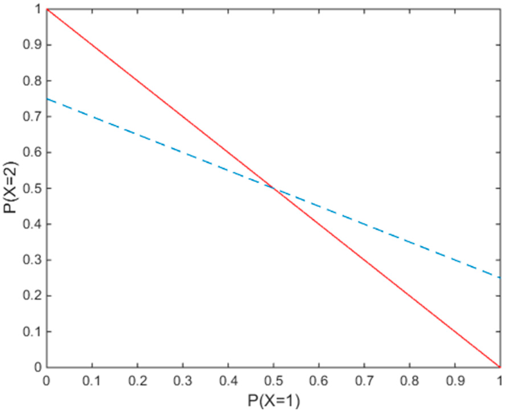
Examining the geometric properties of the solutions to the ME and MLP methods provides further insight to the performance of each. A simple scenario is used for the analysis. The constraint set for both methods creates a bounded polyhedron, a polytope. We consider only constraints on unity and the mean. In the simplest form, if we assume that the random variable has two outcomes: , then the feasible set contains, at most, one point. Figure 1 shows the case where . The only feasible solution for this constraint set is . The dashed line indicates the second constraint, while the solid line refers to the first constraint. Thus, regardless of the objective function, both the ME method and the MLP method will produce the same solution.
6.1. Geometry with a Three-Outcome Variable
The problem becomes more complicated as the number of outcomes increases. For a random variable with three outcomes, the feasible set lies along the intersection of two planes (constraints). The first constraint, , creates a simplex. The second plane, intersects the simplex, creating a line. In general, if , then the line equation for the feasible set can be written as:
For the special case of , the line equation becomes:
For the case where , the line equation becomes , where both methods find the optimal solution at point , or the uniform distribution. Figure 2 shows the line that is formed as the intersection of these two planes for the case where and .
It is very important to understand that is the line equation and not all the points on are feasible. Every element of has to be non-negative and smaller than one, satisfying the probability axioms. For example, in the case of and , the values for can be only be between 0 and 0.5. This observation poses a limitation for the Monte Carlo simulation we discuss next.
6.2. Monte Carlo Simulation
We design a simulation to observe the geometric properties of the solutions of the ME and MLP methods and to locate the solutions on the feasible set (line). We assume that the random variable is discrete with three outcomes . Using the line Equation (22), we modify the mean, and track the changes in the Kullback–Leibler and the total deviation. The algorithm can be summarized as follows:
- The value for is determined: .
- Based on the result of Step 1, the feasible range for is determined using the line equation of Equation (22);
- The value for is incremented by 0.005 from the minimum to the maximum that was computed in the previous step;
- Using the line equation, the values for and are determined;
- is specified as the desired test distribution;
- The optimization problems are solved for and ;
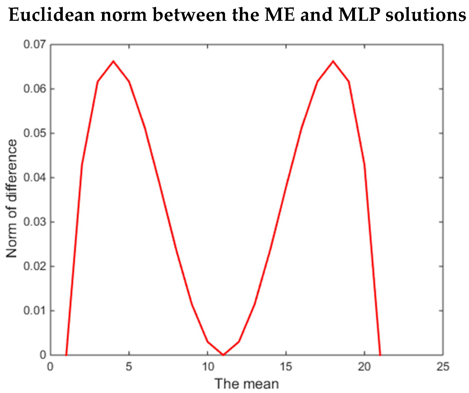
- The Euclidean norm of the difference between the solutions of the ME and MLP methods is calculated:
6.3. Euclidean Distance of the ME and MLP Solutions
Figure 3 shows the Euclidean distance between the solutions of the ME and the MLP methods for every value of the mean, . The distance between the solutions of both methods is the smallest for the boundary cases: or . These instances are the cases with only one feasible solution: and . Hence, the solutions for the ME method and the MLP method are similar. The other minimum occurs in the case of . In this case, the number of points in the feasible set is the maximum possible, but both methods provide the uniform solution: . This solution is what one would expect from the ME method as it is the solution with the maximum uncertainty (i.e., maximum entropy). From these results, we see that the distance between the methods vanishes around the uniform distribution, but increases farther away from it. These results underscore the insights derived previously in this paper showing that there are conditions under which both the ME and MLP methods will produce the same results, and there are also conditions under which the solutions will differ.
7. Conclusions
In this paper, we first reviewed the notion that both ME and MLP methods are specific instantiations of the minimum cross-entropy principle. Through analytic analysis and numerical examples, we then established that the information about the target distribution can significantly affect the performance of the methods. The ME method performs well with exponential distributions, whereas the MLP method has better performance with inverse distributions. We then used the minimum-cross entropy method to generalize the maximum log-probability approach.
The analysis shows that it is not, in general, possible to determine that one method (direction of the Kullback–Leibler divergence) yields better results than the other. Rather, the performance depends on the problem and the information that is available. This work highlights the need to appropriately match the method used to the information available and opens the door to future research on questions such as the performance of these methods in particular contexts and methods to capture all types of available information. We hope this work helps clarify some of the confusion and criticisms of entropy methods and their special cases in the literature. We also hope to see further applications of entropy methods in a variety of applications.
Acknowledgments
This work was supported by the National Science Foundation awards CMMI 15-65168, CMMI 16-29752, and CMMI 16-44991.
Author Contributions
Ali E. Abbas conceived the concept for the paper and contributed to the analytic results. Andrea H. Cadenbach analyzed the results of the simulations and wrote the paper. Ehsan Salimi conducted the simulations and conducted the literature review. All authors have read and approved the final manuscript.
Conflicts of Interest
The authors declare no conflict of interest.
Appendix A
The analytic solutions of MCE. The Lagrangian function for Direction (1) can be written as:
The minimum occurs when the derivative vanishes to zero:
Solving the equation above results in an exponential distribution:
Following the same steps, the solution for Direction (2) can be derived:
MCE solution with a uniform target distribution. Let the target distribution be a uniform distribution, e.g., . Then the Kullback–Leibler divergence for distribution and the uniform distribution as the reference distribution becomes:
where represents the Shannon entropy of the distribution . Hence, minimizing the cross-entropy to the uniform distribution under some given constraints is the same as finding the maximum entropy distribution under the same set of constraints.
MCE solution with a uniform posterior distribution. Suppose ; the Kullback–Leibler divergence in the reverse direction can be written as follows:
The first part of the above expression is constant; hence, minimizing the above expression is similar to maximizing the summation of the natural log of the probabilities, or the objective function of the MLP method:
This result establishes the MLP method as a special case of the minimum relative entropy method with the uniform posterior distribution.
References
- Howard, R.; Abbas, A.E. Foundations of Decision Analysis; Prentice Hall: Upper Saddle River, NJ, USA, 2015. [Google Scholar]
- Box, G.E.; Tiao, G.C. Bayesian Inference in Statistical Analysis; John Wiley & Sons: Hoboken, NJ, USA, 1973. [Google Scholar]
- Jaynes, E.T. Prior Probabilities. IEEE Trans. Syst. Sci. Cybern. 1968, 4, 227–241. [Google Scholar] [CrossRef]
- Nelsen, R.B. An Introduction to Copulas; Springer: New York, NY, USA, 2013. [Google Scholar]
- Abbas, A.E. A Kullback–Leibler view of Linear and Log-Linear Pools. Decis. Anal. 2009, 6, 25–37. [Google Scholar] [CrossRef]
- Montiel, L.V.; Bickel, E.J. Approximating Joint Probability Distributions Given Partial Information. Decis. Anal. 2013, 10, 26–41. [Google Scholar] [CrossRef]
- Rubenstein, R.Y.; Kroese, D.P. The Cross-Entropy Method: A Unified Approach to Combinatorial Optimization, Monte-Carlo Simulation and Machine Learning; Springer: New York, NY, USA, 2004. [Google Scholar]
- Abbas, A.E. Entropy Methods for Univariate Distributions in Decision Analysis. In Bayesian Inference and Maximum Entropy Methods in Science and Engineering; Williams, C., Ed.; American Institute of Physics: Melville, NY, USA, 2002; pp. 339–349. [Google Scholar]
- Abbas, A.E. Entropy Methods for Joint Distributions in Decision Analysis. IEEE Trans. Eng. Manag. 2006, 53, 146–159. [Google Scholar] [CrossRef]
- Abbas, A.E. Maximum Entropy Distributions Between Upper and Lower bounds. In Bayesian Inference and Maximum Entropy Methods in Science and Engineering; Castle, J.P., Morris, R.D., Abbas, A.E., Knuth, K.H., Eds.; American Institute of Physics: Melville, NY, USA, 2005; pp. 25–42. [Google Scholar]
- Abbas, A.E. An Entropy Approach for Utility Assignment in Decision Analysis. In Bayesian Inference and Maximum Entropy Methods in Science and Engineering; Williams, C., Ed.; American Institute of Physics: Melville, NY, USA, 2002; pp. 328–338. [Google Scholar]
- Sonnevend, G. Applications of the notion of analytic center in approximation (estimation) problems. J. Comput. Appl. Math. 1989, 28, 349–358. [Google Scholar] [CrossRef]
- Ye, Y. Interior Point Algorithms: Theory and Analysis; Wiley Interscience: New York, NY, USA, 1997. [Google Scholar]
- Kullback, S.; Leibler, R. On Information and Sufficiency. Ann. Math. Stat. 1951, 22, 79–86. [Google Scholar] [CrossRef]
- Kullback, S. Information Theory and Statistics; Dover Publications: Mineola, NY, USA, 1997. [Google Scholar]
- Boyd, S.; Vandenberghe, L. Convex Optimization; Cambridge University Press: Cambridge, UK, 2004. [Google Scholar]
- Jaynes, E. Information Theory and Statistical Mechanics. Phys. Rev. 1957, 106, 620–630. [Google Scholar] [CrossRef]
- Shannon, C. Communication Theory of Secrecy Systems. Bell Syst. Tech. J. 1949, 28, 656–715. [Google Scholar] [CrossRef]
- Sonnevend, G. An ‘analytical centre’ for polyhedrons and new classes of global algorithms for linear (smooth, convex) programming. In System Modelling and Optimization; Springer: Berlin/Heidelberg, Germany, 1986; pp. 866–875. [Google Scholar]
- Abbas, A.E. Entropy Methods for Adaptive Utility Elicitation. IEEE Trans. Syst. Man Cybern. Part A 2004, 34, 169–178. [Google Scholar] [CrossRef]
Figure 1.
Feasible set for the probability distribution when the variable has two outcomes.

Figure 2.
Feasible set (bold line) when the random variable has three outcomes.
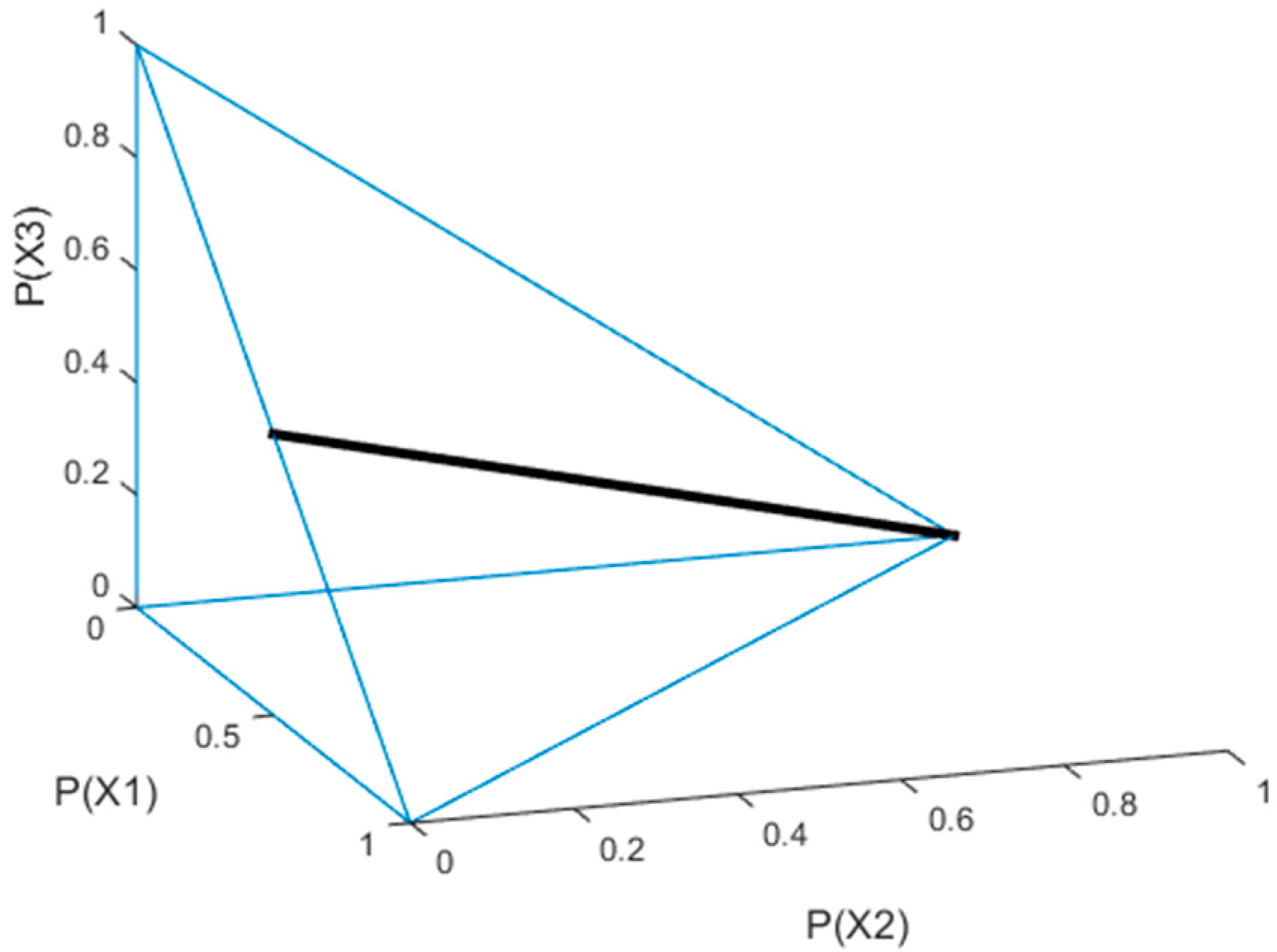
Figure 3.
Euclidean norm of the difference between the ME and MLP solutions.

Table 1.
Univariate first order exponential function with 20 outcomes.
| Divergence Measure | MLP vs. Simulated Distribution | ME vs. Simulated Distribution | ||
|---|---|---|---|---|
| K–L Divergence | Avg. Deviation: 0.315 | Standard Deviation: 0.164 | Avg. Deviation: | Standard Deviation: |
| Total Deviation | Avg. Deviation: 0.588 | Standard Deviation: 0.231 | Avg. Deviation: | Standard Deviation: 0.0002 |
Table 2.
Univariate second order exponential function with 20 outcomes.
| Divergence Measure | MLP vs. Simulated Distribution | ME vs. Simulated Distribution | ||
|---|---|---|---|---|
| K–L Divergence | Avg. Deviation: 0.093 | Standard Deviation: 0.069 | Avg. Deviation: | Standard Deviation: |
| Total Deviation | Avg. Deviation: 0.342 | Standard Deviation: 0.183 | Avg. Deviation: | Standard Deviation: |
Table 3.
Univariate first order rational function with 20 outcomes.
| Divergence Measure | MLP vs. Simulated Distribution | ME vs. Simulated Distribution | ||
|---|---|---|---|---|
| K–L Divergence | Avg. Deviation: | Standard Deviation: | Avg. Deviation: 0.034 | Standard Deviation: 0.017 |
| Total Deviation | Avg. Deviation: | Standard Deviation: | Avg. Deviation: 0.218 | Standard Deviation: 0.069 |
Table 4.
Univariate first-order rational function with 20 outcomes.
| Divergence Measure | MLP vs. Simulated Distribution | ME vs. Simulated Distribution | ||
|---|---|---|---|---|
| K–L Divergence | Avg. Deviation: | Standard Deviation: | Avg. Deviation: 0.0027 | Standard Deviation: 0.0014 |
| Total Deviation | Avg. Deviation: | Standard Deviation: | Avg. Deviation: 0.059 | Standard Deviation: 0.017 |
Table 5.
Comparison of different target functions in Direction (1).
| Divergence Measure | (1) with Exponential Target | (1) with Inverse Target | (1) with Uniform Target | (1) with Uniform Sampling Target |
|---|---|---|---|---|
| K–L Divergence | Average: 0.5153 Standard Deviation: 0.175 | Average: 0.522 Standard Deviation: 0.179 | Average: 0.515 Standard Deviation: 0.1754 | Average: 0.889 Standard Deviation: 0.319 |
| Total Deviation | Average: 0.6944 Standard Deviation: 0.108 | Average: 0.699 Standard Deviation: 0.110 | Average: 0.694 Standard Deviation: 0.108 | Average: 0.948 Standard Deviation: 0.156 |
Table 6.
Comparison of different target functions in Direction (2).
| Divergence Measure | (2) with Exponential Target | (2) with Inverse Target | (2) with Uniform Target | (2) with Uniform Sampling Target |
|---|---|---|---|---|
| K–L Divergence | Average: 0.530 Standard Deviation: 0.181 | Average: 0.545 Standard Deviation: 0.194 | Average: 0.514 Standard Deviation: 0.175 | Average: 0.886 Standard Deviation: 0.320 |
| Total Deviation | Average: 0.708 Standard Deviation: 0.114 | Average: 0.718 Standard Deviation: 0.1205 | Average: 0.693 Standard Deviation: 0.109 | Average: 0.947 Standard Deviation: 0.156 |
Table 7.
Euclidean distance of solutions of both directions.
| Euclidean Norm | Exponential | Inverse | Uniform | Uniform Sampling |
|---|---|---|---|---|
| Uniform sampling Test distribution | 0.0419 (0.028) | 0.033 (0.0337) | 0.0056 (0.0087) | 0.204 (0.0393) |
Table 8.
Performance of MLP vs. generalized MLP methods.
| Divergence Measure | MLP Method | ME Method | ||
|---|---|---|---|---|
| K–L Divergence | Avg. Deviation: 0.314 | Standard Deviation: 0.164 | Avg. Deviation: 0.001 | Standard Deviation: 0.001 |
| Total Deviation | Avg. Deviation: 0.58 | Standard Deviation: 0.227 | Avg. Deviation: 0.034 | Standard Deviation: 0.024 |
© 2017 by the authors. Licensee MDPI, Basel, Switzerland. This article is an open access article distributed under the terms and conditions of the Creative Commons Attribution (CC BY) license (http://creativecommons.org/licenses/by/4.0/).
Share and Cite
MDPI and ACS Style
Abbas, A.E.; H. Cadenbach, A.; Salimi, E. A Kullback–Leibler View of Maximum Entropy and Maximum Log-Probability Methods. Entropy 2017, 19, 232. https://doi.org/10.3390/e19050232
AMA Style
Abbas AE, H. Cadenbach A, Salimi E. A Kullback–Leibler View of Maximum Entropy and Maximum Log-Probability Methods. Entropy. 2017; 19(5):232. https://doi.org/10.3390/e19050232
Chicago/Turabian StyleAbbas, Ali E., Andrea H. Cadenbach, and Ehsan Salimi. 2017. "A Kullback–Leibler View of Maximum Entropy and Maximum Log-Probability Methods" Entropy 19, no. 5: 232. https://doi.org/10.3390/e19050232
Note that from the first issue of 2016, this journal uses article numbers instead of page numbers. See further details here.