
Lyapunov Spectra of Coulombic and Gravitational Periodic Systems

Department of Physics and Astronomy, Texas Christian University, Fort Worth, TX 76129, USA
*
Author to whom correspondence should be addressed.
Entropy 2017, 19(5), 238; https://doi.org/10.3390/e19050238
Submission received: 2 April 2017
/
Revised: 15 May 2017
/
Accepted: 15 May 2017
/
Published: 20 May 2017
(This article belongs to the Special Issue Thermodynamics and Statistical Mechanics of Small Systems)
Abstract
:An open question in nonlinear dynamics is the relation between the Kolmogorov entropy and the largest Lyapunov exponent of a given orbit. Both have been shown to have diagnostic capability for phase transitions in thermodynamic systems. For systems with long-range interactions, the choice of boundary plays a critical role and appropriate boundary conditions must be invoked. In this work, we compute Lyapunov spectra for Coulombic and gravitational versions of the one-dimensional systems of parallel sheets with periodic boundary conditions. Exact expressions for time evolution of the tangent-space vectors are derived and are utilized toward computing Lypaunov characteristic exponents using an event-driven algorithm. The results indicate that the energy dependence of the largest Lyapunov exponent emulates that of Kolmogorov entropy for each system for a given system size. Our approach forms an effective and approximation-free instrument for studying the dynamical properties exhibited by the Coulombic and gravitational systems and finds applications in investigating indications of thermodynamic transitions in small as well as large versions of the spatially periodic systems. When a phase transition exists, we find that the largest Lyapunov exponent serves as a precursor of the transition that becomes more pronounced as the system size increases.
Keywords:
Kolmogorov–Sinai entropy, Lyapunov exponents; periodic boundary conditions; chaotic dynamics; N-body simulation; stochastic thermodynamicsPACS:
52.27.Aj; 05.10.-a; 05.45.Pq; 05.45.Ac; 05.70.Fh1. Introduction
Our understanding of the collective behavior of macroscopic systems is encompassed in the laws of thermodynamics. Phase transitions demonstrate that the state space of macroscopic systems is segmented into regions of strongly differing thermodynamic properties. While phase transitions are rigorously defined in the thermodynamic limit, it is remarkable that their manifestations can sometimes be observed in very small systems (see [1] and references therein). In addition to investigating the occurrence of equilibrium phase transitions, small systems have also been employed to study the breakdown of the second law [2], as well as various equilibrium and nonequilibrium phenomena [3,4,5]. Besides the usual changes in equilibrium properties—such as pressure, energy, and density—at phase transitions typically associated with macroscopic systems, the search for dynamical indicators of phase transitions has also born fruitful results. In particular, in ergodic systems, it has been demonstrated that the largest Lyapunov characteristic exponent (LCE) plays a pivotal role in announcing the existence of a phase transition. While the theory of phase transitions in systems with short-range interactions is well understood, systems with long-range interactions do not satisfy the usual convergence properties [6]. Consequently, surprising behavior, such as ensemble inequivalence, can occur. In contrast with short-range systems, the nature of boundary conditions for long-range systems becomes crucial since the interaction range can be of the same order as that of the system size. In studying possible indicators of phase transitions in small systems, it is useful to know the exact behavior of the system in the thermodynamic limit. One-dimensional systems have proven especially useful in this regard (see [7] for a review of relevant work).
One dimensional systems are of great interest to physicists in terms of their intrinsic properties and as a starting point in the analysis of their more-complicated higher-dimensional counterparts (see [8,9,10,11,12] and references therein). Not only can one-dimensional systems map the behaviors of experimental results [13], one-dimensional interactions have, in fact, been recently emulated in the laboratory [14]. In systems with long-range forces, establishing the exact form of the potential energy is difficult when periodic boundary conditions are involved. In two or three dimensions, Ewald sums are required and the potential cannot be deduced in a closed form. However, in one dimension, it is possible to express the inter-particle potential energy analytically [8]. In the analysis of large systems considered in plasma and gravitational physics, periodic boundary conditions are preferred [15,16,17,18] and have been utilized in the study of one-dimensional Coulombic and gravitational systems [12,19,20,21]. Such studies often rely on numerical simulations to validate the predictions made by theory. Moreover, in cases where theoretical relations have not been mathematically formulated, numerical simulations serve as a powerful approach in characterizing the dynamical behaviors and thermodynamic properties [12].
Simulation studies usually employ the molecular-dynamics (MD) approach for studying dynamical systems that undergo phase-space mixing to exhibit ergodic-like behavior. Phase-space mixing is a necessary condition for equilibrium statistical mechanics to apply and is often characterized by the existence of positive Lyapunov characteristic exponents (LCEs) [22]. LCEs represent the average rates of exponential divergence of nearby trajectories from a reference trajectory in different directions of the phase space and quantify the degree of chaos in a dynamical system [23,24,25,26,27]. In addition, LCEs have also been reported to serve as indicators of phase transitions [28,29,30,31,32,33].
Numerical calculation of LCEs may be realized by studying the geometry of the phase-space trajectories [29,30] for smooth systems. In general, however, if the time evolution of each particles’ position and velocity can be followed for a given system, the largest LCE may be calculated by finding the rate of divergence between a reference trajectory and a nearby test trajectory obtained by pertubing the former [26]. This numerical approach was extended to the case of systems with periodic boundary conditions by Kumar and Miller and was applied to find the largest LCE for a spatially-periodic one-dimensional Coulombic system [12].
While the largest LCE is a good indicator of the degree of maximum dynamical instability in a system, the mixing speed, that is, the rate at which a given phase-space volume element diffuses across the allowed regions of the phase space is indicated by the Kolmogorov–Sinai (KS) entropy. For ergodic-like Hamiltonian systems, KS entropy is obtained as the sum of the positive LCEs [23]. In simulation, a full spectrum of LCEs may be obtained by finding the time-averaged exponential rates of growth of perturbation vectors applied to the phase-space flows in the tangent space [25,34,35,36]. An exact numerical method of calculating the full Lyapunov spectrum was proposed for the case of one-dimensional gravitation gas [25].
Even though a full spectrum of Lyapunov exponents is highly desirable, the calculation becomes computationally challenging for systems with a large number of degrees of freedom and it is usually impractical to aim for a full spectrum through N-body simulations [25]. An improved version of the approach was presented in [37] for the case of free-boundary conditions (also see [38]). In this paper, we extend the numerical approach presented in [25] to compute the complete Lyapunov spectra of spatially-periodic one-dimensional Coulombic and gravitational systems and show that the energy dependence of the largest LCE emulates that of the sum of all the positive LCEs for both versions of the system.
The paper is organized as follows: in Section 2, we describe the Coulombic and gravitational versions of the model and discuss the potential interactions as well as their implications on the phase-space characteristics. In Section 3, we recall some theoretical results for LCEs and the general approach for their numerical computation. Section 4 presents derivations for the time evolution of the tangent vectors and the results of the N-body simulations. Finally, in Section 5, we discuss the results and provide concluding remarks.
2. Model
We consider two versions of a spatially periodic lineal system on an x-axis with the primitive cell extending in and which contains N infinite sheets, each with a surface mass density m. The positions of the sheets are given by with respect to the center of the cell and their corresponding velocities by . In one version, the sheets are uncharged and are only interacting gravitationally. The other version is essentially a one-dimensional Coulombic system in which the sheets are charged with a surface charge density q and are immersed in a uniformly distributed negative background such that the net charge is zero. For the case of the charged version of the system, we neglect the gravitational effects and take into account only the Coulomb interactions. If we denote momenta as , the Hamiltonian of the system may be expressed as
where for the case of the Coulombic system [12] (with each sheet, henceforth referred to as a particle or a body, having a surface charge density q in addition to the surface mass density m) and for the gravitational system [21].
3. Lyapunov Characteristic Exponents
3.1. Theoretical Overview
We provide here a brief overview of dynamical system theory that will be helpful in developing the formulations in subsequent sections. While more general and comprehensive discussions are provided in [25,37,39], we restrict this overview to a smooth Hamiltonian system. We will see later how the concept may be extended to flows that take place on non-differentiable manifolds. Although the mathematical definitions used in the following discussions are rather general, we have adopted—and, for the sake of completion and easy comparison with relevant work, reproduced—their versions as presented in [25,37] unless noted otherwise.
Let the phase-space flow, be a one-parameter group of measure-preserving diffeomorphisms , where M is an n-dimensional compact differentiable manifold and . For a Hamiltonian system with a phase-space dimensionality of , . If is the tangent space to M at z, then we can define as a linearized flow in the tangent space , where w is a vector in the tangent space. For a non-zero w, there are n independent eigenvectors with as the corresponding eigenvalues such that . For a periodic orbit with period , if we define , then
where represents the Euclidean norm on and k is a positive integer [25]. For a tangent-space vector w with a non-zero component along , the divergence for large t will be dominated by , and, therefore,
is usually called the largest Lyapunov characteristic exponent (LCE) of the orbit represented by the flow and is a measure of the overall stability of the orbit; if , then the nearby trajectories diverge exponentially. Note that even though we have used a periodic orbit to define the largest LCE, it may be shown that the limit on the left-hand side of Equation (3) exists and is finite for any given dynamical system and the result applies rather generally under very weak smoothness conditions [40].
LCE defined in Equation (3) may be thought of as the mean exponential growth rate of a one-dimensional “volume” (length of a vector w) in the tangent space. Therefore, is often referred to as an LCE of order 1. Similarly, , that is, LCE of order p (where , ), may be related to the mean exponential rate of growth of a p-dimensional hyperparallelepiped formed by the evolution of p linearly independent tangent-space vectors . We first find the rate of volume divergence as
where represents the volume spanned by a set of p tangent-space vectors. Finally, following [40], is found as
3.2. Numerical Approach
We start with a randomly chosen set of n orthonormal tangent vectors . Clearly, for each , . After a fixed time interval , the evolved tangent vectors—which we denote by , where —are, in general, no longer mutually orthogonal. This is because the component of each along the direction of maximum divergence (that is, ) will witness a disproportionately larger growth in its value as compared to the remaining components. In order to avoid numerical errors arising from one component getting increasingly large in comparison to the others, a new orthonormal set of tangent vectors is defined after time through Gram–Schmidt reduction on the set of evolved . This new set of ornothormal tangent vectors are then used for the following iteration, and the process is recursively repeated until has converged [25,39].
Numerical calculation of involves finding the corresponding p-volume for each iteration. If at the end of the j-th iteration, represents the evolved versions of the orthornormal tangent vectors , the p-volume may be found as the norm of the the exterior product involving the corresponding p vectors, that is,
Finally, the average exponential growth rate of the p-volume is found as
where l is the total number of iterations. A complete set of LCEs , also known as the Lyapunov spectrum, may then be obtained for the trajectory by utilizing Equation (5) for all permissible values of p. Finally, an upper limit on the KS entropy for Hamiltonian systems may be obtained as the sum of positive LCEs [23,25]:
where is the largest value of p for which is positive and where the equality holds for ergodic-like systems. The sum of the positive LCEs is often termed as the density of KS entropy.
In the following section, we discuss how we employ the theory and the numerical approach presented thus far to obtain Lyapunov spectra for the Coulombic and gravitational systems discussed in Section 2. While most of the presented theory applies to the two systems in its original form, non-smoothness arising from the absolute valued linear terms in the potential demand additional consideration. As we shall see, following the time evolution of the tangent-space vectors involves treating the motion as a flow in between two consecutive events of interparticle crossings and as a mapping at each event of such crossings. Consequently, it is indispensable to have the ability to find the exact time corresponding to each crossing.
4. N-Body Simulation
4.1. Equations of Motion
Positions and velocities of the particles are obtained using event-driven algorithms based on the approaches proposed in [12] for the Coulombic system and in [21] for the gravitational system. The algorithms employ analytic expressions for the time dependencies of the relative separations and relative velocities between two consecutive particles in the primitive cell, where and , with and representing, respectively, the position and velocity of the j-th particle, whereas and representing those of the -th particle. Combining the results of [12,21], we find that
Crossing times may be found by solving for t. The corresponding positions and velocities are obtained using a matrix-inversion subroutine as described in [12].
4.2. Time Evolution of Tangent-Space Vectors
In order to follow the time evolution of the tangent vectors, we adopt an approach based on the “exact” numerical method proposed in [25]. The method invokes that, for a one-dimensional Hamiltonian system with N particles, one does not have to restrict to the -dimensional manifold . One may alternatively choose to represent the flow in the entire -dimensional phase space (say, ) whereby the tangent space becomes a subspace of .
Let be a point in the phase space , where and . The equations of motion representing the system are given by
and
with
Similarly, if we have a vector in the tangent space , then the variational equations [25] governing the evolution of w are given by
where is the identity matrix and is an matrix whose elements are given by
For the potential expressed in Equation (12), one finds that
Time evolution of between the events of interparticle crossings may be deduced by adding Equation (19) for all values of j as
which implies that
Hence, in between the events of crossings, the evolution of tangent vectors takes the form
With the two values of , one for the Coulombic system and the other for the gravitational system, one may solve Equation (24) to find the exact dependencies of and on time.
4.2.1. Coulombic System
Utilizing the initial conditions for the Coulombic system with , we obtain the solutions to Equation (24) for and in between crossings as
and,
where .
If the r-th and s-th particles undergo a crossing at time , and and , respectively, denote the instants just before and after , then
4.2.2. Gravitational System
For the gravitational system, . Similar to the Coulombic case, we utilize the initial conditions to find solutions to Equation (24) for and as functions of time for the gravitational case in between the events of crossings:
where,
and . For the r-th and s-th particle involved in a crossing, we get
where we have used the same definitions of , , and as we did in the expressions’ Coulombic counterparts.
4.3. p-Volume and Lyapunov Spectrum
We perform numerical computations using algorithms that are driven by tracking the events of interparticle crossings. Since the time derivatives of the velocities of the particles involved in a crossing undergo abrupt changes, tracking of crossing becomes indispensable. In other words, even if we were to sample the positions and velocities at fixed intervals of time, we would still need to track every crossing [25]. Therefore, instead of choosing fixed time intervals for Gram–Schmidt orthonormalization of the tangent-space vectors, we choose to do it after each crossing. It should be noted that the duration of each iteration, fixed or variable, is irrelevant as long it remains short enough for the various components of the tangent vectors to remain comparable with a given precision offered by the computing platform utilized.
After an iteration, say, the -th iteration, ending at time , each of the orthonormal tangent vectors is allowed to evolve for the duration of the j-th iteration. may be thought of as the time elapsed between the instants right after the -th crossing and right before the j-th crossing. Then, the evolved vectors may be given by , where
For the j-th iteration, p-volume is found as follows: we define a symmetric matrix whose elements are inner products between and , where (with ). That is,
The matrix , also referred to as Gram matrix, encapsulates the necessary geometric information about the subspace spanned by the set of vectors such as the lengths of the vectors and the angles between them. The absolute value of the determinant of , known as the Gramian, is essentially the square of the norm of the exterior product [41]. Using Equation (6), the p-volume is found as
With the ability to find each p-volume for a given iteration, the final value of the corresponding are found as
where , as defined in Equation (35), is the total time elapsed for l crossings to occur. Finally, LCEs and Kolmogorov-entropy density are obtained using Equations (5) and (8), respectively.
4.4. Results
In our simulation, the initial conditions are chosen as follows: for a given number of particles N and per-particle energy , if is lower than the maximum allowed value of the potential energy , then the particle positions are chosen randomly such that the potential energy is slightly smaller than the target value of . For greater than , the particle positions are randomly selected such that the potential energy is close to . Velocities are chosen randomly from a Gaussian distribution and are scaled such that the sum of the potential and kinetic energies exactly equals the target value of [12].
Simulations are performed by rescaling the system parameters using dimensionless units such that the number density and the characteristic frequencies , equal unity [12,21]. Energies and (respectively for Coulombic and gravitational systems) are measured with respect to the minimum values of the corresponding potential energies allowed for each N.
Before running the Lyapunov algorithm, we allowed the system to evolve for a relaxation period of 500 time units (in terms of or ). In the calculation of LCEs, the total number of iterations l for each in Equation (38) is decided by an adaptive algorithm that runs a minimum preliminary number of iterations assigned beforehand and then continues running until the value of has converged to within a pre-specified tolerance for the standard deviation. The tolerance value that we specified was percent of the mean from the newest iterations, with a minimum of 1 million iterations. In each run, we found that the values converged to within our specified tolerance after the preliminary run of 1 million iterations.
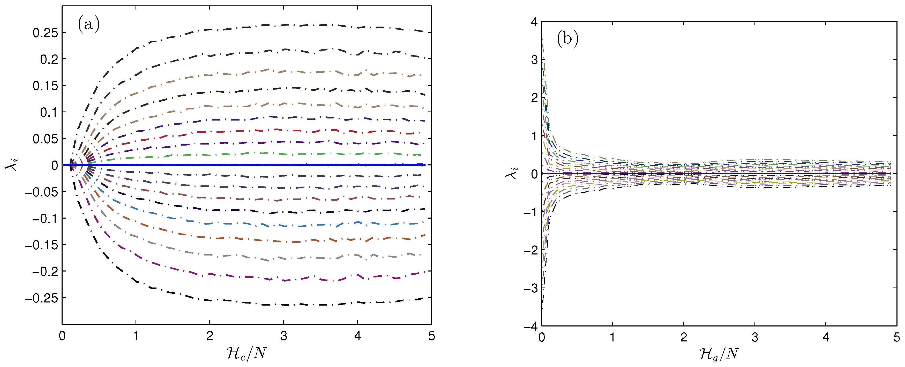
We computed Lyapunov spectra for the Coulombic and gravitational systems with a varying number of particles N with . Figure 1 shows examples of the dependence of the various LCEs on the per-particle energy for the Coulombic and gravitational systems with . The figure also shows the sum of all LCEs for each case. As expected, the sums were found to be close to zero. It should be noted that versions of the systems with may exhibit largely segmented phase-space distributions with a coexistence of chaotic and stable regions for a given energy value ( being purely trivial with completely integrable phase space) [11,12,25,42]. Hence, there is a considerable probability that a randomly chosen initial condition ends up in one of the stable regions whose trajectories exhibit no stochasticity and which results in values of LCEs close to zero in simulation.
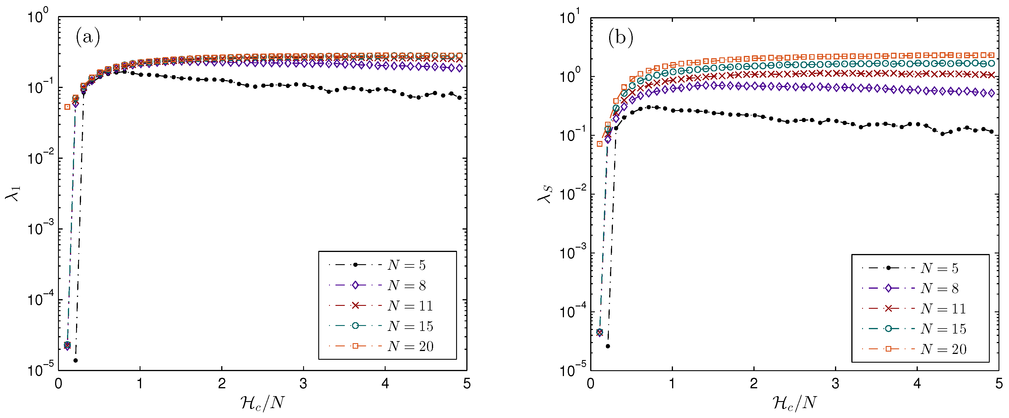
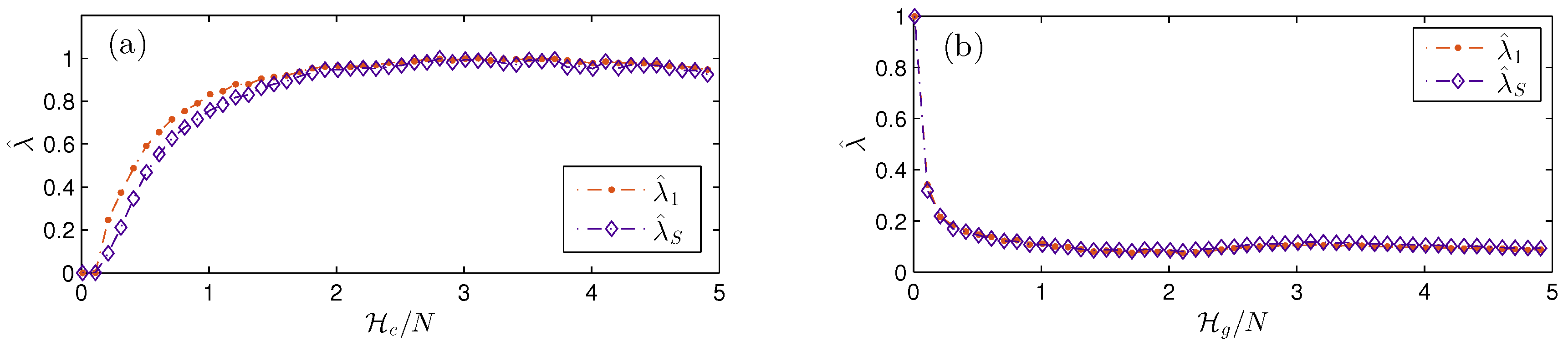
The energy dependencies of the largest LCE and the Kolmogorov-entropy density with and 20 have been shown for the Coulombic and gravitational systems in Figure 2 and Figure 3, respectively. It can be seen in each case that the behavior of versus resembles, in general, a scaled version of versus . To elucidate this, we have presented comparative plots of the normalized versions, and , of and against per-particle energy for in Figure 4, where we have divided and by their respective maximum values to get the normalized values.
5. Discussion
Our study provides insight into the chaotic dynamics of the two versions of the periodic system under conditions of varying energy and degrees of freedom. The results for the Coulombic system are consistent with those provided in [12]. for the Coulombic system stays zero as long as the energy is low enough for the particles to not undergo crossings. As the energy is increased from a low value, sees an initial increase, reaches a maximum and then decreases as the energy is progressively raised. However, with an increase in the number of particles, the right edge of the “hill” near the maximum opens up to form a “plateau” and flattens out asymptotically as shown in Figure 2a. Interestingly, our results also suggest that all the other LCEs are, more or less, scaled (and inverted, for the case of negative LCEs) versions of the largest LCE, as we can see in Figure 1a for N = 11.
Unlike the Coulombic version, the gravitational system shows a maximum degree of chaos at low energies. Our results suggest that the largest LCE starts off with a high value at low energies and decreases to a minimum as the energy is increased for a given N. With further rise in energy, increases, reaches a maximum and then decreases asymptotically. As the number of particles is increased, the local trough near the local minimum and the hill near the local maximum start opening up to the right with the asymptotic edge rising up to a form a plateau as shown in Figure 3b. Moreover, it can also be seen in Figure 3b that the local minimum and maximum themselves shift to the right as well with an increase in the number of particles. It should be noted that, in the thermodynamic limit, that is, for versions of the system with sufficiently large N, the LCEs may exhibit discontinuities in their values or their slopes near the troughs and crests when plotted against temperature. Such an observation may indicate toward the existence of phase transitions [31,32].
While the energy dependencies of differs dramatically for each version of the system, the other LCEs for the gravitational system are also, in general, scaled versions of , similar to the Coulombic system, as exemplified in Figure 1b for N = 11. Moreover, in both versions of the spatially-periodic system, the energy dependence of LCEs tends to approach a common limiting behavior as N is increased. This is in contrast to the free-boundary gravitating case in which the values of LCEs were shown to increase linearly with an increase in the number of particles [25].
From a dynamical perspective, the results are consistent with the theoretical predictions for Hamiltonian systems [25] as outlined below:
- (a)
- The sum of LCEs was found to converge to zero for all energies and N.
- (b)
- For the ordered set (), the results show that
- (c)
- In addition, our results show that
Result (c) is nothing but a consequence of the conservation of momentum [25].
To summarize, we have provided an exact method to compute the full spectra of LCEs for the spatially periodic versions of the one-dimensional Coulombic and gravitational systems. Analytic expressions for the time evolution of the tangent vectors were derived and used in numerically computing LCEs using an efficient event-driven algorithm. While the resulting values of the largest LCE for the Coulombic system agree with those reported previously [12], our exact approach offers striking advantages over the method used in [12] in that it allows one to calculate a full spectrum of LCEs rather than just the largest LCE. Second, the results of the exact method do not depend on the size of the perturbation. In finding the largest LCE using finite perturbations to a reference orbit as discussed in [12], one has to first make sure that the value chosen for initial perturbation is small enough. This becomes challenging for systems in which particles tend to stay clumped together. An example of such behavior is seen in the gravitational system at low energies. Finally, the exact approach circumvents the need for defining a test trajectory altogether, which, as discussed in [12], poses difficulties in expressing phase-space separations for systems with periodic boundary conditions. Nevertheless, the method discussed in [12] still remains powerful, and perhaps the only resort, in dealing with spatially-periodic systems for which analytic evolution of tangent-space vectors may not be obtained.
In our exposition, we started with the general mathematical definitions for the computation of Lyapunov exponents arising in nonlinear dynamics that have been known for quite some time. We subsequently developed those general analytic expressions to account for the particular changes brought upon by the introduction of periodic boundary conditions. As it became evident early in the treatment, the resulting mathematical relations, although somewhat reminiscent of those arrived at in [25] in their differential form, are considerably more complex in their final form.
The results of our study further indicate that the energy dependence of the largest LCE captures the general behavior of the dependence of the Kolmogorov-entropy density on energy for both Coulombic and gravitational systems. This result is particularly significant because of the numerical difficulties encountered while calculating the full Lyapunov spectra of large systems. For the two versions of the spatially-periodic system, our study suggests that one may gain insights into the full spectrum of LCEs by simply looking at the largest LCE, thereby allowing one to avoid the computational complications faced when calculating a full spectrum. Note that this is in contrast with the recent study of Lyapunov spectra in the HMF model [43]. A possible explanation lies in the fact that, unlike the HMF model, the systems considered in the present work are truly one-dimensional and rigorously obey Poisson’s equation [21].
It should be noted that, for a given number of particles, the energy dependence of the LCEs roughly followed the same behavior for any randomly selected initial conditions with only slight deviations. As the number of particles was increased, the deviations became smaller, leading the behaviors to converge to a single universal one, suggesting that the systems approach ergodicity. Moreover, the convergence times of the LCNs for different randomly-chosen initial conditions also showed uniformity for a larger number of particles, thereby pointing toward a consistent relaxation to equilibrium with increasing degrees of freedom. However, the exact dependence of relaxation time on the number of particles requires further investigation and we plan to pursue it in our future work.
Finally, it is worth emphasizing that if a phase transition occurs in either of the two spatially-periodic systems, the temperature dependence of the largest LCE is expected to show a transitioning behavior in the thermodynamic limit (large-N limit) [31,32,44]. Although of only technical interest for short-range interactions, boundary conditions have a strong influence on the behavior of matter for long-range interactions. In a related work [7], we showed, using both mean field theory as well as the simulation approach presented in this paper, the occurrence of a phase transition in a spatially-periodic, one-dimensional gravitational system. It should be noted that no phase transition occurs in the free-boundary version of the same system. For the periodic case studied here with finite N, it turns out that the local peak observed in the largest LCE is the precursor of the phase transition. When plotted versus temperature, this precursor transforms into a cusp characterized by a discontinuity of slope for the gravitational system in the thermodynamics limit [7]. Similar behavior was reported for a self-gravitating ring system [33]. However, as conjectured by Kunz [19], no such transitioning behavior is indicated for the Coulombic system. As we mentioned earlier, the ability to emulate a many body, one-dimensional, gravitational system in the laboratory is a recent development [14]. As experimental techniques progress, it may become possible to control the type of boundary conditions employed in the laboratory. This offers the promise of experimentally observing the phase transition that we predicted in our recent work [7].
Acknowledgments
The authors thank Harald Posch of the University of Vienna and Igor Prokhorenkov of Texas Christian University for valuable insights and helpful discussions.
Author Contributions
Pankaj Kumar and Bruce Miller made contributions to the conception of the research project and formulation of its scope; Pankaj Kumar carried out mathematical derivations, algorithm development, numerical simulations, data acquisition, and data analysis; Pankaj Kumar drafted the paper; Bruce Miller revised the paper critically for relevant background content and added important scientific remarks concerning the behaviors exhibited by the results.
Conflicts of Interest
The authors declare no conflict of interest.
Abbreviations
The following abbreviations are used in this manuscript:
| LCE | Lyapunov characterstic exponent |
| KS | Kolmogorov–Sinai |
| MD | Molecular dynamics |
| HMF | Hamiltonian Mean Field |
References
- Klinko, P.; Miller, B.N. Dynamical study of a first order gravitational phase transition. Phys. Lett. A 2004, 333, 187–192. [Google Scholar] [CrossRef]
- Wang, G.; Sevick, E.M.; Mittag, E.; Searles, D.J.; Evans, D.J. Experimental demonstration of violations of the second law of thermodynamics for small systems and short time scales. Phys. Rev. Lett. 2002, 89, 050601. [Google Scholar] [CrossRef] [PubMed]
- Bustamante, C.; Liphardt, J.; Ritort, F. The nonequilibrium thermodynamics of small systems. Phys. Today 2005, 58, 43–48. [Google Scholar] [CrossRef]
- Ritort, F. The nonequilibrium thermodynamics of small systems. C. R. Phys. 2007, 8, 528–539. [Google Scholar] [CrossRef]
- Schnell, S.K.; Vlugt, T.J.; Simon, J.M.; Bedeaux, D.; Kjelstrup, S. Thermodynamics of a small system in a μT reservoir. Chem. Phys. Lett. 2011, 504, 199–201. [Google Scholar] [CrossRef]
- Frisch, H.L.; Lebowitz, J.L. The Equilibrium Theory of Classical Fluids: A Lecture Note and Reprint Volume; WA Benjamin: Los Angeles, CA, USA, 1964. [Google Scholar]
- Kumar, P.; Miller, B.N.; Pirjol, D. Thermodynamics of a one-dimensional self-gravitating gas with periodic boundary conditions. Phys. Rev. E 2017, 95, 022116. [Google Scholar] [CrossRef] [PubMed]
- Rybicki, G.B. Exact statistical mechanics of a one-dimensional self-gravitating system. Astrophys. Space Sci. 1971, 14, 56–72. [Google Scholar] [CrossRef]
- Yawn, K.R.; Miller, B.N. Equipartition and Mass Segregation in a One-Dimensional Self-Gravitating System. Phys. Rev. Lett. 1997, 79, 3561–3564. [Google Scholar] [CrossRef]
- Miller, B.N.; Youngkins, P. Phase Transition in a Model Gravitating System. Phys. Rev. Lett. 1998, 81, 4794–4797. [Google Scholar] [CrossRef]
- Lauritzen, A.; Gustainis, P.; Mann, R.B. The 4-body problem in a (1+1)-dimensional self-gravitating system. J. Math. Phys. 2013, 54, 072703. [Google Scholar] [CrossRef]
- Kumar, P.; Miller, B.N. Chaotic dynamics of one-dimensional systems with periodic boundary conditions. Phys. Rev. E 2014, 90, 062918. [Google Scholar] [CrossRef] [PubMed]
- Milner, V.; Hanssen, J.L.; Campbell, W.C.; Raizen, M.G. Optical Billiards for Atoms. Phys. Rev. Lett. 2001, 86, 1514–1517. [Google Scholar] [CrossRef] [PubMed]
- Chalony, M.; Barré, J.; Marcos, B.; Olivetti, A.; Wilkowski, D. Long-range one-dimensional gravitational-like interaction in a neutral atomic cold gas. Phys. Rev. A 2013, 87, 013401. [Google Scholar] [CrossRef]
- Springiel, V.; Frenk, C.S.; White, S.D.M. The large-scale structure of the universe. Nature 2006, 440, 1137–1144. [Google Scholar] [CrossRef] [PubMed]
- Bertschinger, E. Simulations of structure formation in the universe. Annu. Rev. Astron. Astrophys. 1998, 36, 599–654. [Google Scholar] [CrossRef]
- Hockney, R.W.; Eastwood, J.W. Computer Simulation Using Particles; CPC Press: Boca Raton, FL, USA, 1988. [Google Scholar]
- Hernquist, L.; Bouchet, F.R.; Suto, Y. Application of the Ewald method to cosmological N-body simulations. Astrophys. J. Suppl. 1991, 75, 231–240. [Google Scholar] [CrossRef]
- Kunz, H. The one-dimensional classical electron gas. Ann. Phys. 1974, 85, 303–335. [Google Scholar] [CrossRef]
- Schotte, K.D.; Truong, T.T. Phase transition of a one-dimensional Coulomb system. Phys. Rev. A 1980, 22, 2183–2188. [Google Scholar] [CrossRef]
- Miller, B.N.; Rouet, J.L. Ewald sums for one dimension. Phys. Rev. E 2010, 82, 066203. [Google Scholar] [CrossRef] [PubMed]
- Krylov, N.; Migdal, A.; Sinai, Y.G.; Zeeman, Y.L. Works on the Foundations of Statistical Physics by Nikolai Sergeevich Krylov; Princeton Series in Physics; Princeton University Press: Princeton, NJ, USA, 1979. [Google Scholar]
- Pesin, J.B. Characteristic Liapunov indices and ergodic properties of smooth dynamical systems with invariant measure. Sov. Math. Dokl. 1976, 17, 196. [Google Scholar]
- Pesin, Y.B. Characteristic Lyapunov exponents and smooth ergodic theory. Russ. Math. Surv. 1977, 32, 55–114. [Google Scholar] [CrossRef]
- Benettin, G.; Froeschle, C.; Scheidecker, J.P. Kolmogorov entropy of a dynamical system with an increasing number of degrees of freedom. Phys. Rev. A 1979, 19, 2454–2460. [Google Scholar] [CrossRef]
- Ott, E. Chaos in Dynamical Systems; Cambridge University Press: Cambridge, UK, 2002; pp. 137–145. [Google Scholar]
- Sprott, J. Chaos and Time-Series Analysis; Oxford University Press: Oxford, UK, 2003; pp. 116–117. [Google Scholar]
- Butera, P.; Caravati, G. Phase transitions and Lyapunov characteristic exponents. Phys. Rev. A 1987, 36, 962–964. [Google Scholar] [CrossRef]
- Caiani, L.; Casetti, L.; Clementi, C.; Pettini, M. Geometry of Dynamics, Lyapunov Exponents, and Phase Transitions. Phys. Rev. Lett. 1997, 79, 4361–4364. [Google Scholar] [CrossRef]
- Casetti, L.; Pettini, M.; Cohen, E.G.D. Geometric approach to Hamiltonian dynamics and statistical mechanics. Phys. Rep. 2000, 337, 237–341. [Google Scholar] [CrossRef]
- Dellago, C.; Posch, H.A. Lyapunov instability, local curvature, and the fluid-solid phase transition in two-dimensional particle systems. Phys. A Stat. Mech. Appl. 1996, 230, 364–387. [Google Scholar] [CrossRef]
- Barre, J.; Dauxois, T. Lyapunov exponents as a dynamical indicator of a phase transition. Europhys. Lett. 2001, 55, 2. [Google Scholar] [CrossRef]
- Monechi, B.; Casetti, L. Geometry of the energy landscape of the self-gravitating ring. Phys. Rev. E 2012, 86, 041136. [Google Scholar] [CrossRef] [PubMed]
- Dellago, C.; Posch, H. Kolmogorov-Sinai entropy and Lyapunov spectra of a hard-sphere gas. Phys. A Stat. Mech. Appl. 1997, 240, 68–83. [Google Scholar] [CrossRef]
- Milanović, L.; Posch, H.A.; Thirring, W. Statistical mechanics and computer simulation of systems with attractive positive power-law potentials. Phys. Rev. E 1998, 57, 2763–2775. [Google Scholar] [CrossRef]
- Tsuchiya, T.; Gouda, N. Relaxation and Lyapunov time scales in a one-dimensional gravitating sheet system. Phys. Rev. E 2000, 61, 948–951. [Google Scholar] [CrossRef]
- Benettin, G.; Galgani, L.; Giorgilli, A.; Strelcyn, J.M. Lyapunov Characteristic Exponents for smooth dynamical systems and for hamiltonian systems; a method for computing all of them. Part 1: Theory. Meccanica 1980, 15, 9–20. [Google Scholar] [CrossRef]
- Shimada, I.; Nagashima, T. A numerical approach to ergodic problem of dissipative dynamical systems. Prog. Theor. Phys. 1979, 61, 1605–1616. [Google Scholar] [CrossRef]
- Sandri, M. Numerical calculation of Lyapunov exponents. Math. J. 1996, 6, 78–84. [Google Scholar]
- Oseledec, V.I. A multiplicative ergodic theorem. Lyapunov characteristic numbers for dynamical systems. Trans. Mosc. Math. Soc. 1968, 19, 197–231. [Google Scholar]
- Shilov, G.E.; Silverman, R.A. An Introduction to the Theory of Linear Spaces; Dover: Mineola, NY, USA, 2012. [Google Scholar]
- Kumar, P.; Miller, B.N. Dynamics of Coulombic and gravitational periodic systems. Phys. Rev. E 2016, 93, 040202. [Google Scholar] [CrossRef] [PubMed]
- Ginelli, F.; Takeuchi, K.A.; Chaté, H.; Politi, A.; Torcini, A. Chaos in the Hamiltonian mean-field model. Phys. Rev. E 2011, 84, 066211. [Google Scholar] [CrossRef] [PubMed]
- Bonasera, A.; Latora, V.; Rapisarda, A. Universal Behavior of Lyapunov Exponents in Unstable Systems. Phys. Rev. Lett. 1995, 75, 3434–3437. [Google Scholar] [CrossRef] [PubMed]
Figure 1.
Full spectra of Lyapunov characteristic exponents (LCEs) plotted against per-particle energy for (a) Coulombic system, and (b) gravitational system, with . The topmost curve shows , the second to top curve shows , and so on all the way to the curve on the very bottom representing in (a,b). The central solid (blue) line in each plot shows the sum of LCEs. and are expressed in units of . are expressed in units of (a) , and (b) .

Figure 2.
Energy dependence of (a) the largest LCE, and (b) Kolmogorov-entropy density for Coulombic system with different degrees of freedom. and are expressed in units of , whereas is expressed in units of .
Figure 2.
Energy dependence of (a) the largest LCE, and (b) Kolmogorov-entropy density for Coulombic system with different degrees of freedom. and are expressed in units of , whereas is expressed in units of .

Figure 3.
Energy dependence of (a) the largest LCE, and (b) Kolmogorov-entropy density for gravitational system with different degrees of freedom. and are expressed in units of , whereas is expressed in units of .
Figure 3.
Energy dependence of (a) the largest LCE, and (b) Kolmogorov-entropy density for gravitational system with different degrees of freedom. and are expressed in units of , whereas is expressed in units of .
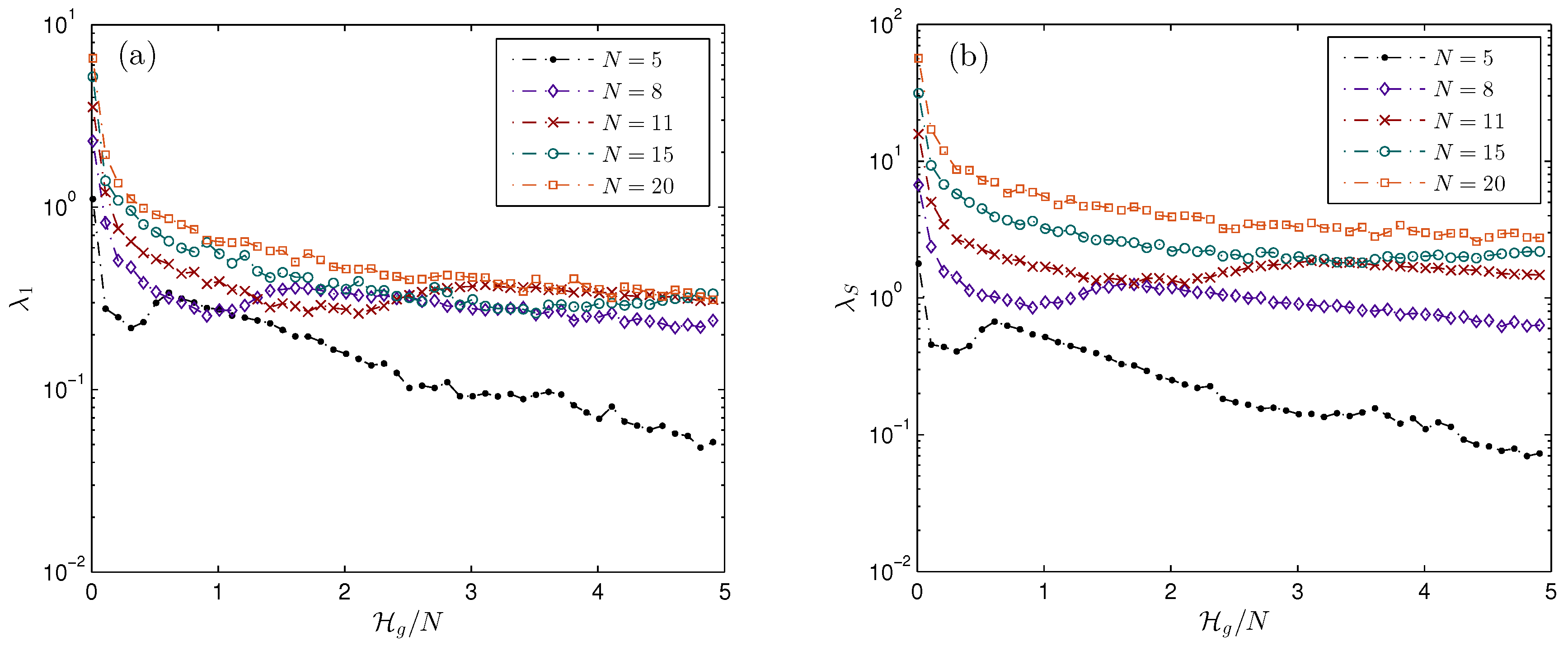
Figure 4.
Energy dependence of the normalized values of the largest LCE and Kolmogorov-entropy density for (a) Coulombic system, and (b) gravitational system for . and are expressed in units of , whereas is dimensionless.
Figure 4.
Energy dependence of the normalized values of the largest LCE and Kolmogorov-entropy density for (a) Coulombic system, and (b) gravitational system for . and are expressed in units of , whereas is dimensionless.
© 2017 by the authors. Licensee MDPI, Basel, Switzerland. This article is an open access article distributed under the terms and conditions of the Creative Commons Attribution (CC BY) license (http://creativecommons.org/licenses/by/4.0/).
Share and Cite
MDPI and ACS Style
Kumar, P.; Miller, B.N. Lyapunov Spectra of Coulombic and Gravitational Periodic Systems. Entropy 2017, 19, 238. https://doi.org/10.3390/e19050238
AMA Style
Kumar P, Miller BN. Lyapunov Spectra of Coulombic and Gravitational Periodic Systems. Entropy. 2017; 19(5):238. https://doi.org/10.3390/e19050238
Chicago/Turabian StyleKumar, Pankaj, and Bruce N. Miller. 2017. "Lyapunov Spectra of Coulombic and Gravitational Periodic Systems" Entropy 19, no. 5: 238. https://doi.org/10.3390/e19050238
Note that from the first issue of 2016, this journal uses article numbers instead of page numbers. See further details here.