
Multiscale Entropy Analysis of the Differential RR Interval Time Series Signal and Its Application in Detecting Congestive Heart Failure


School of Control Science and Engineering, Shandong University, Jinan 250061, China
*
Authors to whom correspondence should be addressed.
Entropy 2017, 19(6), 251; https://doi.org/10.3390/e19060251
Submission received: 21 March 2017
/
Revised: 19 May 2017
/
Accepted: 25 May 2017
/
Published: 31 May 2017
(This article belongs to the Special Issue Entropy and Cardiac Physics II)
Abstract
:Cardiovascular systems essentially have multiscale control mechanisms. Multiscale entropy (MSE) analysis permits the dynamic characterization of the cardiovascular time series for both short-term and long-term processes, and thus can be more illuminating. The traditional MSE analysis for heart rate variability (HRV) is performed on the original RR interval time series (named as MSE_RR). In this study, we proposed an MSE analysis for the differential RR interval time series signal, named as MSE_dRR. The motivation of using the differential RR interval time series signal is that this signal has a direct link with the inherent non-linear property of electrical rhythm of the heart. The effectiveness of the MSE_RR and MSE_dRR were tested and compared on the long-term MIT-Boston’s Beth Israel Hospital (MIT-BIH) 54 normal sinus rhythm (NSR) and 29 congestive heart failure (CHF) RR interval recordings, aiming to explore which one is better for distinguishing the CHF patients from the NSR subjects. Four RR interval length for analysis were used (, and ). The results showed that MSE_RR did not report significant differences between the NSR and CHF groups at several scales for each RR segment length type (Scales 7, 8 and 10 for , Scales 3 and 10 for , Scales 2 and 3 for both and ). However, the new MSE_dRR gave significant separation for the two groups for all RR segment length types except at Scales 9 and 10. The area under curve (AUC) values from the receiver operating characteristic (ROC) curve were used to further quantify the performances. The mean AUC of the new MSE_dRR from Scales 1–10 are 79.5%, 83.1%, 83.5% and 83.1% for , , and , respectively, whereas the mean AUC of MSE_RR are only 68.6%, 69.8%, 69.6% and 67.1%, respectively. The five-fold cross validation support vector machine (SVM) classifier reports the classification Accuracy () of MSE_RR as 73.5%, 75.9% and 74.6% for , and , respectively, while for the new MSE_dRR analysis accuracy was 85.5%, 85.6% and 85.6%. Different biosignal editing methods (direct deletion and interpolation) did not change the analytical results. In summary, this study demonstrated that compared with MSE_RR, MSE_dRR reports better statistical stability and better discrimination ability for the NSR and CHF groups.
Keywords:
multiscale entropy; heart rate variability; congestive heart failure; sample entropy; cardiovascular time seriesPACS:
87.85.Ng; 05.45.Tp; 87.19.Hh; 87.19.ug; 87.19.uj1. Introduction
Short-term, beat-to-beat cardiovascular variability reflects the inherent interactions from different components of cardiovascular system and dynamic interplay between ongoing perturbations to the circulation and compensatory response of neurally mediated regulatory mechanisms [1]. Heart rate variability (HRV) analysis is a prerequisite for understanding the underlying signal generating mechanisms and detecting the cardiovascular diseases [2]. Congestive heart failure (CHF) is a typical degeneration of the heart function featured by the reduced ability for the heart to pump blood efficiently [3]. It is a difficult condition to manage in clinical practice, and the mortality from CHF is high [4,5,6,7,8].
HRV analysis has given an insight into understanding the abnormalities of CHF, and can be used to identify the higher-risk CHF patients [9,10,11,12,13]. Depressed HRV has been used as a risk predictor in CHF [14,15,16]. CHF patients usually have a higher sympathetic and a lower parasympathetic activity [15,16]. Typical HRV analysis for CHF patients include the following publications: Nolan et al. found that the standard deviation of RR interval time series (SDNN) was the most powerful predictor of the risk of death for CHF disease [5]. Binkley et al. reported that parasympathetic withdrawal, in addition to the augmentation of sympathetic drive, is an integral component of the autonomic imbalance characteristic for CHF patients and can be detected noninvasively by HRV spectral analysis [16]. Rovere et al. reported that the low frequency (LF) component was a powerful predictor of sudden death in CHF patients [17]. Hadase et al. also confirmed that the very low frequency (VLF) content was a powerful predictor [18]. Woo et al. demonstrated that Poincare plot analysis is associated with marked sympathetic activation for heart failure patients and may provide additional prognostic information and an insight into autonomic alterations and sudden cardiac death [15]. Guzzetti et al. found significantly lower normalized LF power and lower 1/f slope in CHF patients compared with controls. Moreover, the patients who died during the follow-up period presented further reduced LF power and steeper 1/f slope than the survivors [19]. Yu and Lee used the bispectral analysis and genetic algorithm (GA) for CHF recognition [10]. Makikallio et al. showed that a short-term fractal scaling exponent was the strongest predictor of mortality of CHF [20]. Poon and Merrill found that the short-term variations of beat-to-beat interval exhibited strongly and consistently chaotic behavior in all healthy subjects but were frequently interrupted by periods of seemingly non-chaotic fluctuations in patients with CHF [14]. Peng et al. used fractal dimension analysis (FDA) analysis and confirmed a reduction in HR complexity in CHF patients [21]. All those studies have verified that decreased HRV was associated with the increased mortality in CHF patients. In addition, Jong et al. reported the optimal timing to screen CHF patients and normal sinus rhythm (NSR) subjects was found to be from 7:00 p.m. to 9:00 p.m. during the circadian observation [12]. By using feature selection and classifier optimization, CHF patients can be identified from the NSR group by different combination of time-domain, frequency-domain and non-linear indices [9,11].
In recent years, entropy-based measures, such as the typical approximate entropy (ApEn) [22] and sample entropy (SampEn) [23], have been widely used in HRV analysis. Entropy refers to the degree of regularity or irregularity of a time series and is estimated by counting how many “template” patterns repeat. Repeated patterns imply increased regularity in the time series and lead to low entropy values. SampEn is regarded as a modified version of ApEn to solve the shortcomings, such as bias and relative inconsistency [23]. However, the traditional SampEn method is single-scale based and, therefore, fails to account for the multiple time scales inherent in cardiovascular systems [24,25,26]. Thus, Costa et al. proposed a multiscale entropy (MSE) method for the multiscale analysis [26] and it has received much attention in the biomedical and mechanical fields [27,28,29]. MSE was further developed for multiscale multivariate entropy analysis [27,29,30,31,32,33]. Existing entropy-based CHF studies include: Liu et al. reported decrease of ApEn values in CHF group [34]. Liu et al. also developed a fuzzy measure entropy (FuzzyMEn) method for the normal/CHF classification [35]. Zhao et al. systematically compared the effects of entropy parameters on CHF identification [36]. Costa et al. used MSE for classifying CHF patients and healthy subjects, and reported that the best discrimination between CHF and healthy heart rate (HR) signals with Scale 5 in the MSE calculation [26,37,38]. Kumar et al. used accumulated fuzzy entropy (AFEnt) and accumulated permutation entropy (APEnt) for automated detection of CHF in flexible analytic wavelet transform framework based on short-term HRV signals [13]. In addition, recently, von Tscharner and Zaniyeh used a multiscale transitions of fuzzy SampEn to diagnose CHF patients from normal subjects and reported a sensitivity of 87% and a specificity of 89% [39].
MSE method employs an entropy measure to quantify the degree of unpredictability of time series derived from the original signal by coarse-graining, which divide the original signal into non-overlapping segments of equal length and calculating the mean value of the data points in each of these segments as the coarse-grained signal. As the variant versions, in 2009, Valencia et al. proposed a refined MSE version (RMSE) [40]. In 2013, Wu et al. proposed a composite multiscale entropy (CMSE) [41] and, in 2015, proposed a refined CMSE (RCMSE) [42]. In 2015, Costa et al. also developed a generalization for their MSE analysis to quantify the dynamics of the volatility (variance) of a signal over multiple time scales and performed on the CHF analysis [43].
Intuitively, the MSE and its variant versions directly process the original RR interval time series as a coarse graining. There have also been nonlinear analysis reported for the differential RR interval time series signal (i.e., the signal increment series), rather than the original RR interval time series. In these studies, this difference signal was decomposed into magnitude and sign series, and the results verified that the magnitude series relates to the non-linear properties of the original RR time series, while the sign series relates to the linear properties [44,45,46,47]. In addition, both magnitude and sign series verified the clinical values using a detrended fluctuation analysis (DFA) method. Thus, in this study, we will perform the MSE method on the differential RR interval time series signal. An unaddressed question is whether only using the single property of the data, i.e., the original RR time series, to derive the entropy values at different scales, discards important information whose quantification could enhance the identification ability for CHF. To help address this question, we herein develop an MSE analysis, which uses the differential signal of the original RR interval time series rather than the original RR interval time series themselves, for the coarse-graining procedure. We denote the new MSE analysis for the differential RR interval time series signal as MSE_dRR and the MSE analysis for the original RR interval time series as MSE_RR.
Thus, the main goal of the present study is to carry out an in depth analysis on MSE_RR and MSE_dRR, to explore which one is better for distinguishing the CHF patients from the normal sinus rhythm (NSR) subjects using the long-term MIT-Boston’s Beth Israel Hospital (MIT-BIH) RR Interval Databases [48]. The rest of the paper is organized as follows. Section 2 details the method descriptions, including the database, the calculations of MSE_RR and MSE_dRR, and the statistical and evaluation methods. Section 3 presents the results for MSE_RR and MSE_dRR. Finally, Section 4 draws the discussions and identifies the limitations and future work.
2. Methods
2.1. Data
All data used were from the MIT-BIH RR Interval Databases from http://www.physionet.org [48], a free-access, on-line archive of physiological signals. The NSR RR Interval Database was used as the non-pathological and control group data. This database included 54 long-term RR interval recordings of subjects in normal sinus rhythm aged 29 to 76. The CHF RR Interval Database was used as the pathological group data. This database included 29 long-term RR interval recordings of subjects aged 34 to 79, with congestive heart failure (NYHA classes I, II, and III). The original electrocardiography (ECG) signals for both NSR and CHF RR interval databases were digitized at 128 Hz, and the beat annotations were obtained by automated analysis with manual review and correction.
2.2. Method Description
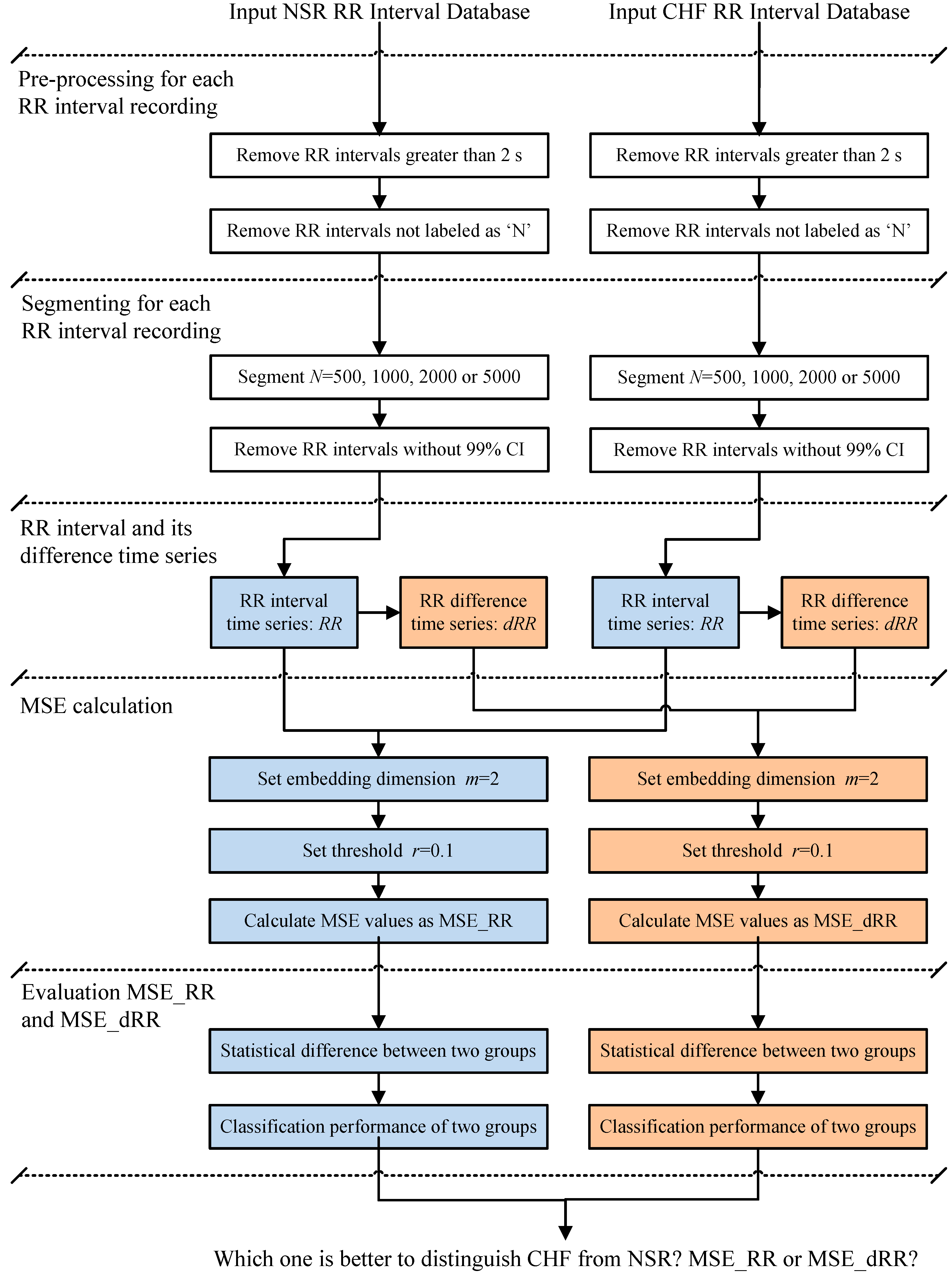
Figure 1 shows the block diagram of the analytical procedure used in the present study. This procedure consisted of five major steps: Step 1, Pre-processing for each RR interval recording; Step 2, Segmenting for each RR interval recording; Step 3, Difference time series calculation for each RR segment; Step 4, MSE calculation; and, Step 5, Statistical and evaluation methods.
In Step 1, the RR intervals greater than 2 s were firstly removed from the original RR interval recordings to ignore the influence from the artifacts. For each beat in the raw ECG signals, it was annotated as a normal (denoted as “N”) or abnormal heartbeat. The abnormal heartbeats were usually caused by the ectopic beats such as supra-ventricular ectopic beats or ventricular ectopic beats, depending on the localization of the ectopic focus. The RR intervals formed from the abnormal heartbeats could confound the entropy analysis of HRV [49]. Thus, these RR intervals were then removed from the RR interval recordings. Table 1 shows the total number of RR intervals for both NSR and CHF groups, as well as the numbers of RR intervals after these two removing procedures. The percentages of the reserved RR intervals after the removal are 99.1% and 93.7% for NSR and CHF groups respectively.
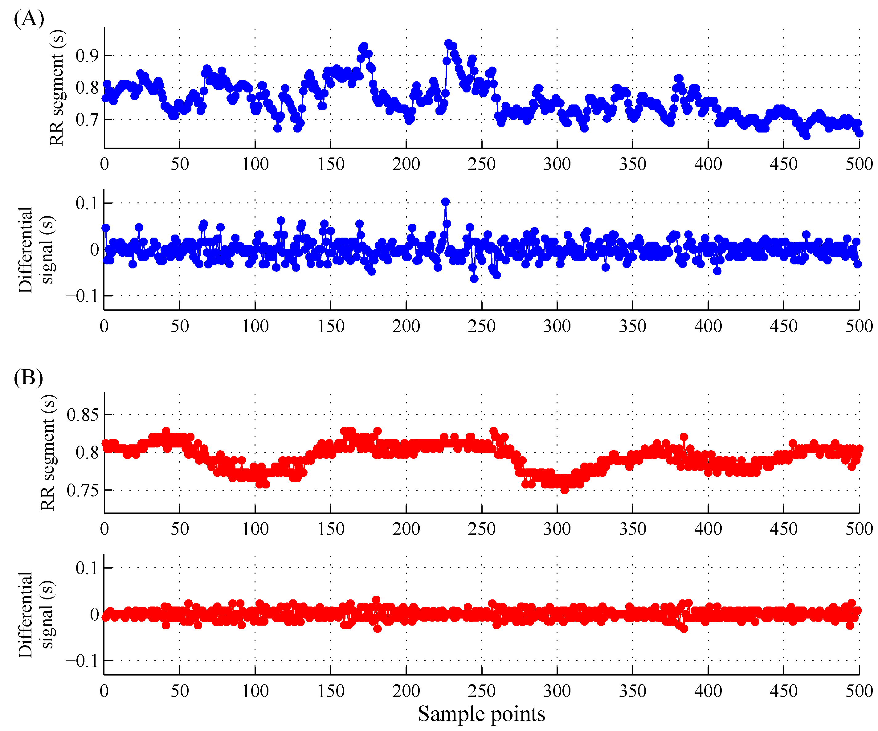
In Step 2, we used four different length windows N to segment the long-term RR interval recordings to form the RR segments for MSE calculation. Since the data length is crucial in the calculation of MSE [50,51,52], we performed the segmentation procedure after the removal of the abnormal heartbeat to keep both NSR subjects and CHF patients have the similar RR segment lengths when using a special segmentation window size. We did not consider the overlapping operation between adjacent -length windows. In this study, we set , , and , respectively, to observe the performances of MSE results for different RR time series lengths. Table 1 also shows the total numbers of RR segments for both NSR and CHF groups when setting , , and , respectively. For each RR segment, we finally removed the RR intervals without 99% confidence interval (CI). Figure 2 shows the examples of RR segments of the two groups.
In Step 3, the difference time series was calculated from the original RR segment as:
where is time series length. Both time series were input into the next Step for MSE calculation.
In Step 4, MSE was used to calculate the entropy values for each RR segment (MSE_RR) and its difference time series (MSE_dRR), using Scales 1–10. The other parameter settings were: embedding dimension and tolerance threshold suggested in [36]. The detailed descriptions of MSE_RR and MSE_dRR methods were summarized in the next section.
In Step 5, firstly, the entropy results of MSE_RR and MSE_dRR were statistically compared between the NSR and CHF groups. The statistical methods are summarized in Section 2.4. Then, in order to test the classification ability of the new MSE_dRR, we performed the receiver operating characteristic (ROC) curve analysis and the classification accuracy detection based on support vector machine (SVM) K-fold cross validation.
For ROC analysis, a cut-point was established and the individual MSE value on one side of the cut-point is labeled as NSR subject and that with value on the other side is labeled as CHF patient. The ROC curve is a plot of (Sensitivity) versus (1-Specificity) at all possible threshold . The possible threshold values varied from the minimum to the maximum of the MSE_RR or MSE_dRR outputs, with a step of 1% of the range of the entropy results. Sensitivity and Specificity were defined as:
where TP is the number of the CHF patients were correctly classified as the CHF group, TN is the number of the NSR subjects were correctly classified as the NSR group, FP is the number of the NSR subjects were falsely classified as the CHF group, and FN is the number of the CHF patients were falsely classified as the NSR group. The common index of area under curve (AUC) was used to evaluate the classification performances of MSE_RR and MSE_dRR, aiming to explore MSE_RR and MSE_dRR, which one is better for distinguishing the CHF patients from the NSR subjects.
Sensitivity: Se = TP/(TP + FN)
Specificity: Sp = TN/(TN + FP)
For SVM-based classification accuracy detection, we used the MSE values from the 10 scales as the individual SVM vector input, and used five-fold cross validation, i.e., all 54 NSR and 29 CHF subjects were randomly divided into five folds. All subjects except the current fold ones were used to train the SVM model and each fold subjects were used as test set for NSR/CHF classification. We used the libsvm software package to learn the SVM models [53]. The default parameter settings of libsvm were used: radial basis function as kernel function, gamma parameter γ in kernel function as 0.1, cost parameter as 2. Three indices were used for performance evaluation: sensitivity, specificity and accuracy. Sensitivity and specificity are defined in Equations (2) and (3). Accuracy was defined as:
where TP, FN, FP and TN have the same meanings with the definitions under Equations (2) and (3).
Accuracy: Acc = (TP + TN)/(TP + FN + FP + TN)
2.3. Multiscale Entropy (MSE)
Step 1: A coarse-graining procedure to derive a time series representing the inherent dynamic on different time scales. The coarse-graining procedure for Scale is obtained by averaging the data points of the time series inside consecutive but non-overlapping windows of length . Thus for the original RR segment and its difference time series , the coarse-grained time series and are computed using Equations (5) and (6), respectively:
where means the rounding down and represents the scale factor. For Scale 1, the coarse-grained time series and corresponds to the original RR segment and its difference time series.
Step 2: SampEn is calculated for each coarse-grained time series and at each scale. Sample entropy is a conditional probability measure that quantifies the likelihood that a vector of consecutive data points that matches another vector of the same length (match within a tolerance of ) will still match the other vectors when their length is increased of one sample (vectors of length ); therefore defines the length of the patterns that are compared to each other [23]. In this definition, the distance between two vectors is computed as the maximum absolute difference of their corresponding scalar components [23]. More precisely, sample entropy is determined as
where is the probability that two vectors will match for points and is the probability that two vectors will match for points (both with a tolerance of and the self-matches are excluded). Equation (7) is estimated by the statistics [23]
2.4. Statistical Analysis
For one NSR or CHF RR interval recording (i.e., one subject), there will be multiple RR segments, and thus will be multiple MSE_RR and MSE_dRR values. Their averages of MSE_RR and MSE_dRR values are calculated as the individual results. Then, mean ± standard deviation (SD) of the two MSE results were obtained across all NSR subjects and CHF patients. The MSE results were tested as normal distribution by the Kolmogorov–Smirnov test. If the MSE results met the normal distribution, the group t-test was used to test the statistical difference between the NSR and CHF groups. If not, non-parametric test was used. All statistical analyses were performed using the SPSS software (Ver. 20, IBM, New York, NY, USA). Statistical significance was set a priori at p < 0.01.
3. Results
3.1. Statistical Differences of MSE_RR and MSE_dRR between the Two Groups
All MSE_RR and MSE_dRR results, from both NSR and CHF groups, had normal distribution from the Kolmogorov–Smirnov test. Table 2 gives their overview results for the two groups when using the segment lengths of , , and , respectively. The MSE results without statistical differences between the two groups were marked as gray shadows. For any combination of parameter setting, both MSE_RR and MSE_dRR results were consistently lower in the CHF group than those in the NSR group.
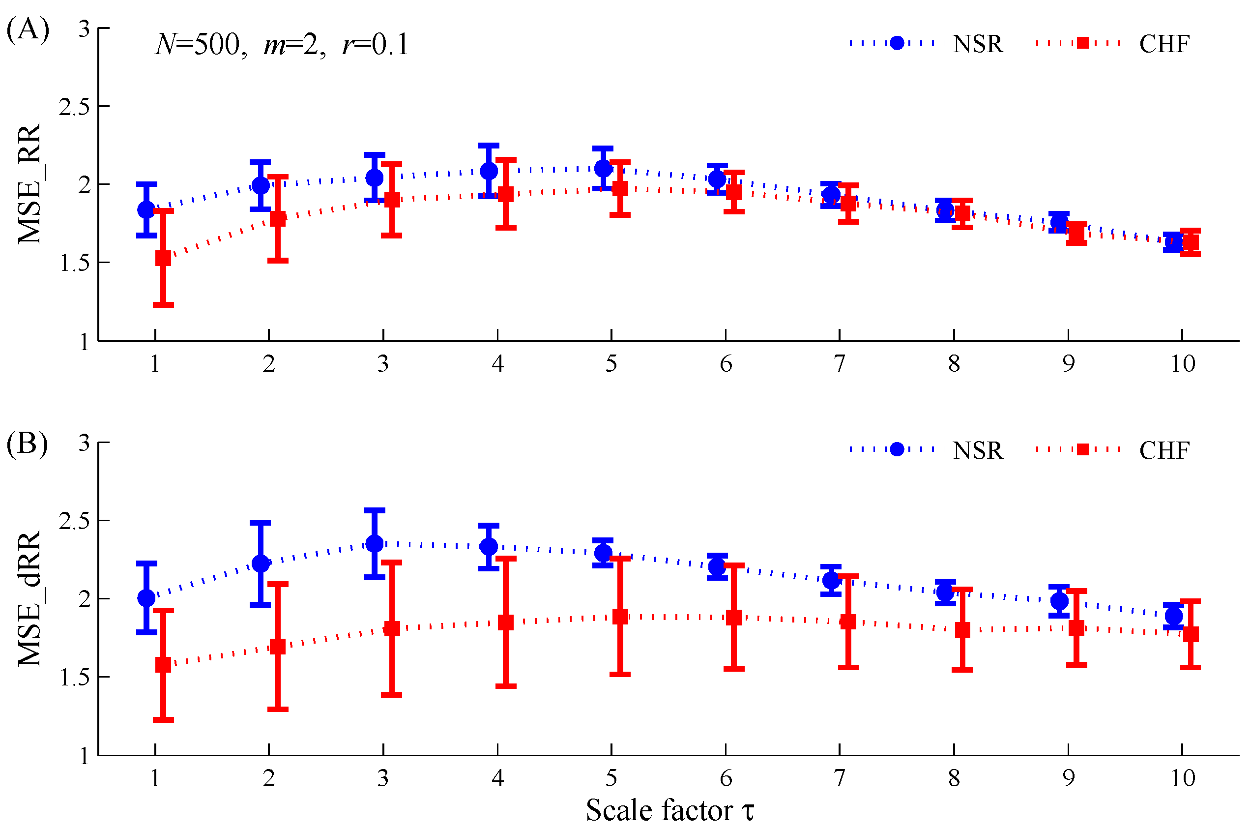
When using , MSE_RR did not report significantly lower values in the CHF group than those in the NSR group for Scales 7, 8 and 10, while MSE_dRR also did not report significantly lower values in the CHF group for Scales 9 and 10 (see Figure 3). When using , MSE_RR did not report significantly lower values in the CHF group than those in the NSR group for Scales 3 and 10. However, when performing the MSE_dRR analysis on the difference signal of RR interval time series, significantly lower values were found in the CHF group for all 10 used scales. Moreover, MSE_dRR differences between the two groups were more statistically significant than MSE_RR results (see Figure 4). The statistical significances for MSE_dRR at the 10 scales were all smaller than 10−8 whereas they were all larger than 10−8 for MSE_RR.
3.2. Classification Results Using ROC Curve Analysis
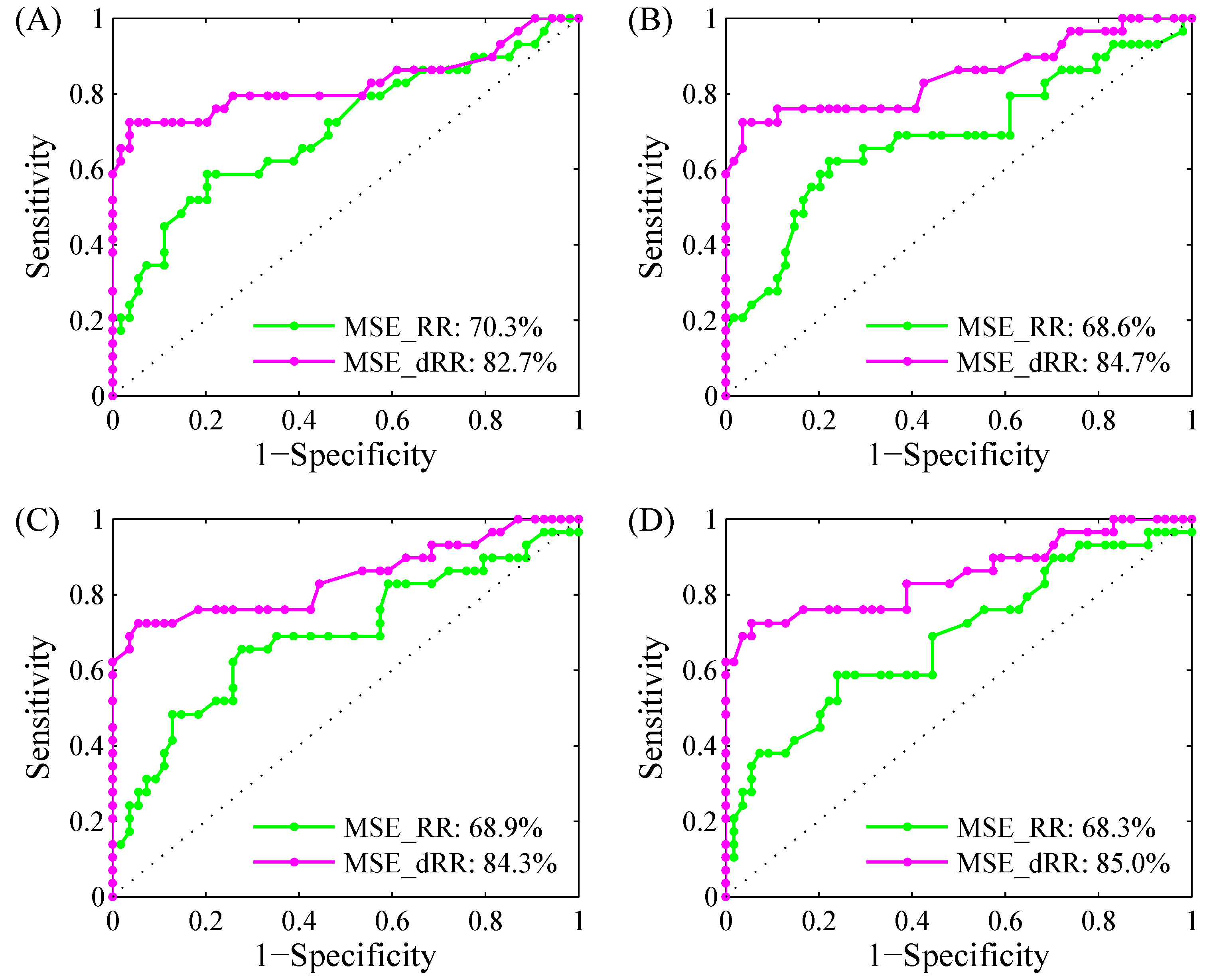
Figure 7 shows the examples of ROC curve plots with AUC values for MSE_RR and MSE_dRR results for classifying NSR and CHF groups under four RR segment length types. Scale 4 was used. Table 3 gives all AUC results for MSE_RR and MSE_dRR for Scales 1–10.
For classifying NSR and CHF groups, the new MSE_dRR always had larger AUC values than MSE_RR for all RR segment length type. The mean values of MSE_dRR from Scales 1–10 are 79.5%, 83.1%, 83.5% and 83.1% for , , and , respectively, whereas the mean values of MSE_RR are only 68.6%, 69.8%, 69.6% and 67.1%, respectively. MSE_dRR gives an improvement for the NSR/CHF classification performance by enhancing the mean AUC values of 10.9%, 13.3%, 13.9% and 16.0% for the four RR segment length types, respectively. Meanwhile, as shown in Table 3, no matter , , , or , the AUC values from MSE_RR changed obviously for different scales. However, the AUC values from MSE_RR kept at a relatively stable level. The MSE_RR SD results from the 10 scales were far larger than those in MSE_dRR method and were 11.0%, 5.1%, 4.8% and 5.5%, respectively. However, they were only 7.1%, 2.1%, 0.7% and 1.2%, respectively, for MSE_dRR. In addition, it is worth noting that the SD results from both MSE_RR and MSE_dRR are extremely large (11.0% and 7.1%, respectively) when . The reason is that there are lots of “No values (NaN)” MSE values exist at large scales when using small RR segment length of .
3.3. Classification Results Using 5-Fold Cross Validation SVM Classifier
Table 4 shows the five-fold cross validation SVM classifier results on all 54 NSR and 29 CHF subjects, at three RR segment length types: , and . was not evaluated since there are lots of “NaN” values for both MSE_RR and MSE_dRR at this RR segment length type, resulting the failing of training SVM models. For , the mean , and of MSE_RR from 5 folds are 70.1%, 75.7% and 73.5%, respectively. MSE_dRR gives better classification results of 86.2%, 85.2% and 85.5% for , and respectively. and report similar results with . The mean , and of MSE_RR are 72.9%, 77.2% and 75.9% for , and 72.9%, 75.0% and 74.6% for , respectively. As comparison, the mean , and of MSE_dRR are larger and report the same results of 84.4%, 86.8% and 85.6% for both and , respectively. It is worth noting that both MSE_RR and MSE_dRR output similar and values because all SVMs were learned to maximize the value while including a parameter to encourage the and to be equal.
.
3.4. Comparison of Different Editing Methods for Abnormal RR Intervals
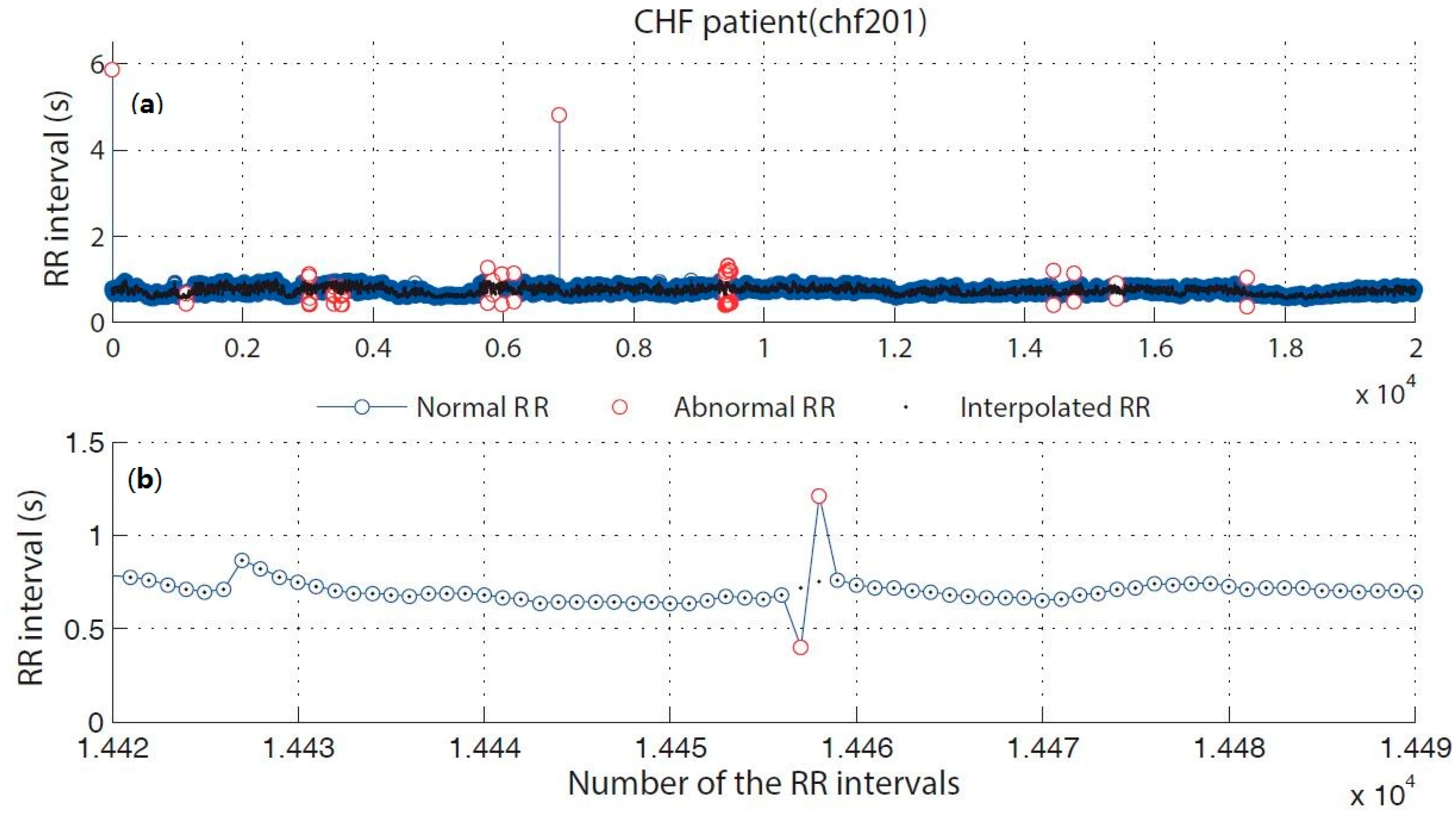
Abnormal RR intervals were directly deleted in the first Step of the proposed analytical procedure. Herein, we compared two editing methods for abnormal RR intervals: the direct deletion method and the interpolation method. Figure 8 shows the examples of the original RR interval time series and the interpolated RR time series for correcting the abnormal RR intervals. As shown in Table 1, when using a time length of , after directly deleting the abnormal RR intervals, there are 5711 and 3089 RR segments reserved for NSR and CHF groups, respectively. In contrast, when the abnormal RR intervals were interpolated, the number of the RR segments increased to 5760 and 3296 for NSR and CHF groups respectively. Table 5 shows the results of MSE_RR and MSE_dRR () for the NSR and CHF groups respectively when analyzing the interpolated RR segments. Similar to the results from the RR segments with abnormal RR interval deletion, both MSE_RR and MSE_dRR results were consistently lower in the CHF group than those in the NSR group. MSE_RR did not report significantly lower values in the CHF group than those in the NSR group for Scales 3, 9 and 10. However, MSE_dRR reported significantly lower values in the CHF group compared to the NSR group for all 10 used scales.
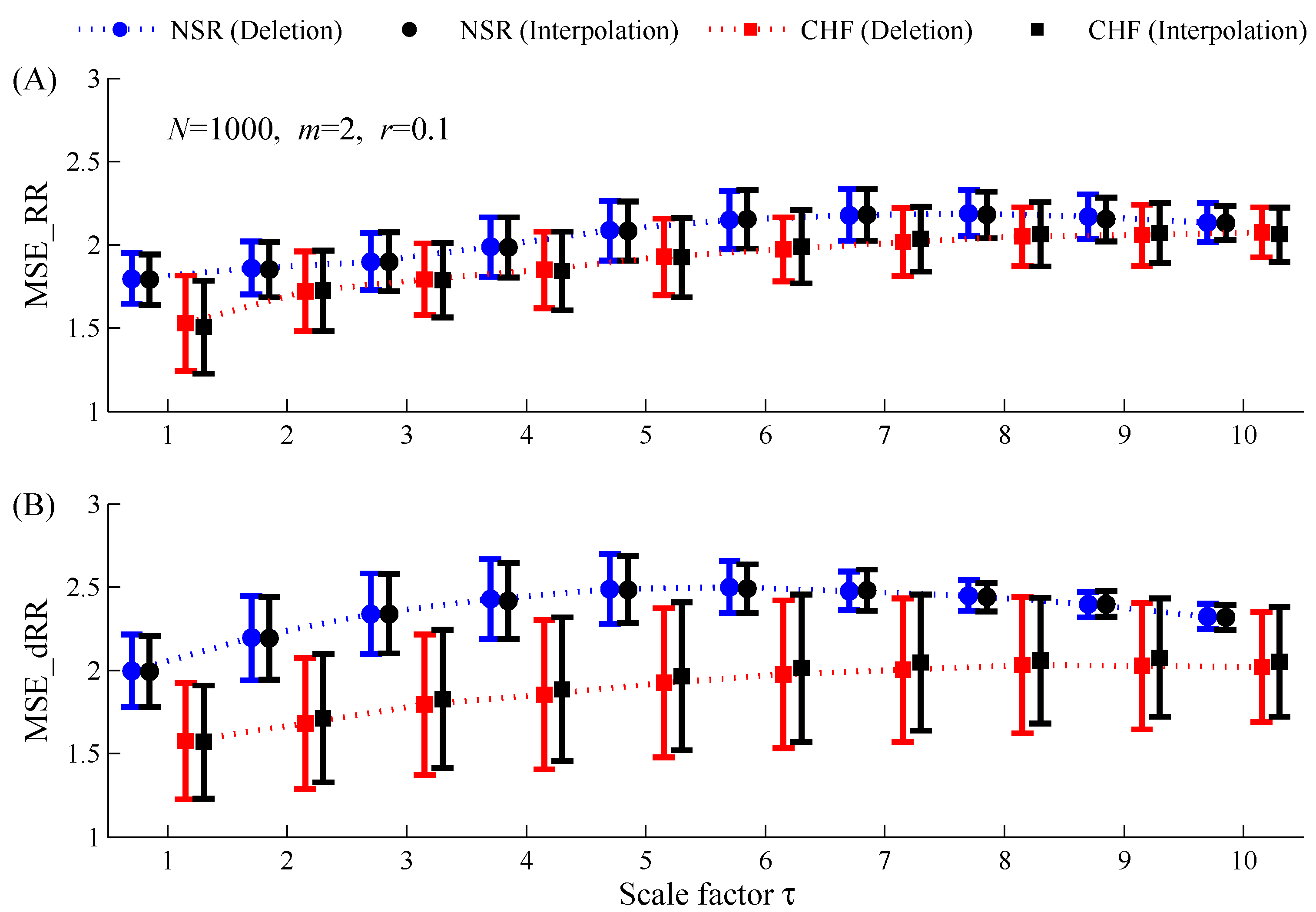
Figure 9 gives the MSE results on the RR time series () using two editing methods for the abnormal RR intervals (the direct deletion method and the interpolation method) respectively. For either NSR or CHF group, paired-t test results showed that both MSE_RR and MSE_dRR reported no significant statistical differences between the direct deletion method and the interpolation method.
.
4. Discussions
This study proposed a new insight for multisacle entropy analysis, which performed the traditional MSE method on the differential RR interval time series signal (named as MSE_dRR analysis) rather than on the original RR segments (named as MSE_RR analysis). As an application, the new MSE_dRR, as well as MSE_RR, have been applied to test the discrimination ability between NSR subjects and CHF patients. This study showed that, with the new MSE_dRR, the classification performances between NSR subjects and CHF patients were significantly enhanced compared with the traditional MSE_RR analysis. The better discrimination ability of MSE_dRR were confirmed from the analysis of four RR segment length types (, , and ) on the widely used MIT-BIH NSR and CHF RR Interval Databases, with a total of more than 9 million of RR intervals. From five-fold cross validation, the traditional MSE_RR achieves a 73.5% accuracy while MSE_dRR achieves an 85.5% accuracy on an length RR time series, with a sensitivity of 86.2% and a specificity of 85.2%. This classification accuracy (85.5%) is comparable to the classification result reported in [39], which showed a sensitivity of 87% and a specificity of 89%. It is worth noting that we did not perform any optimization for the five-fold cross validation SVM method and we used the default parameter setting in the libsvm software [53]. The classification accuracy of 85.5% in MSE_dRR can be expected to enhance if the SVM optimization is involved. One possible explanation for the better performance of the new MSE_dRR is that the signal drift in the original RR segment has been removed in the differential signal.
A possible explanation for why the dynamics of the differential RR interval time series signal (first derivative dRRI) gives more information than the original RR interval time series is important. From a physiological viewpoint, the rhythm of the heart is an essential non-linear system, which is characterized by a non-linear, non-stationary property of the RR interval. The dynamics of the RR interval time series is due to the result of two competing forces, the sympathetic and parasympathetic activities [44,47], which possess long-range correlations with scale-invariant structure. Detecting and quantifying the non-linear property of RR interval time series is of great importance. The non-linear property can be depicted by the original RR interval time series, or from its differential signal, i.e., its increments . The differential signal is more relevant than the series itself because its dynamical properties can provide interesting clues about the underlying dynamics of the system and can help to develop useful models [44]. Previous studies showed that the magnitude series generated from the differential signal relates to the nonlinear properties of the original RR time series, while the sign series generated from the differential signal relates to the linear properties [44,45,46,47], indicating that the non-linear properties are included in the differential signal of RR time series. The inherent physiological mechanism is reflected by the differentiated time series is the sympathetic activity, which is responsible to the small changes in magnitude of the differential signal, while the parasympathetic activity is usually associated with fast increases of the RR interval, responding to the large changes in magnitude of the differential signal. We identified the direct link between the magnitude information in the differential signal of the original RR time series and the nonlinear property in cardiovascular system as the possible reason for the better performance of MSE_dRR analysis in this study.
In addition, previous studies have shown that the drift in RR intervals can disturb the SampEn computation [24,39], and thus result in the poor SampEn statistical stability [35,54,55]. The fuzzy function-based entropy methods were proposed as they are less sensitive to drift in the RR time series because the mean is subtracted from the time series leading to more stable results [35,39,55]. Herein, the MSE_dRR analysis has a similar effect with the fuzzy function-based entropy methods and gives new insight for entropy applications.
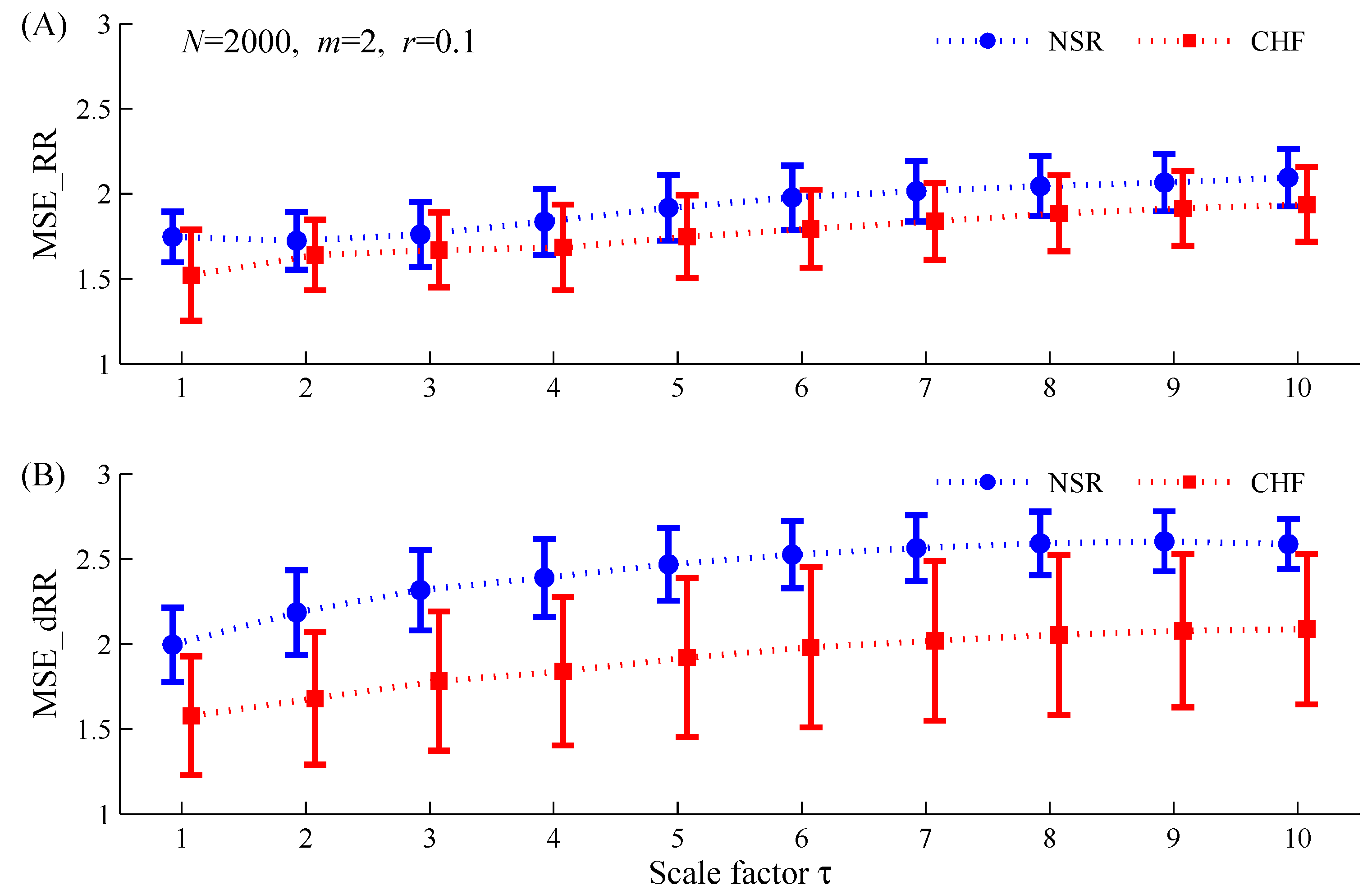
Cardiovascular systems essentially have multiscale control mechanisms. Unlike the single scale analysis of SampEn, MSE analysis permits the dynamic characterization of the cardiovascular time series for both short-term and long-term processes, and thus can be more illuminating. Previous findings using MSE showed that complexity degrades in CHF patients [26,37,38]. In the present study, as shown in Figure 3, Figure 4, Figure 5 and Figure 6, MSE analysis for the original RR segment, i.e., MSE_RR, although had the capacity to distinguish the CHF patients from the NSR subjects at the majority of scale factors, it still failed at some scales, especially at small scales. This is consist with the previous results [26,38]. In contrast, the new MSE_dRR analysis showed the much better statistical separations between the two groups, suggesting that we should pay more attention on the differential signal of the RR interval time series. In addition, the parameter setting for entropy methods should be cautious. There is no generalized guidelines exist for selecting the appropriate entropy parameters of , and . Zhao et al. systematically tested the different parameter combinations of and for SampEn and confirmed that the typically recommended values between 0.1 and 0.25 and in the literature [56] did not always generate significant separation for the two groups. The parameter combination of and could work but not for the parameter combination of and [36]. Thus, extreme caution should be paid when choosing appropriate parameters for distinguishing CHF patients from NSR subjects. In this study, although we used the better parameter combination of and , the MSE_RR results still did not reveal the separation ability for the two groups at several specific scales.
The discrimination ability of MSE_dRR for NSR and CHF groups is quantified by the AUC values from ROC curve analysis. As shown in Table 3, its classification performance for CHF is consistently better than the traditional MSE_RR analysis under any of the four RR segment lengths. Since the new MSE_dRR analysis only adds a step for the difference calculation for the original RR interval time series, it is conceptually simple and computationally efficient, allowing it to be potentially useful in a real time context. The new MSE_dRR seems to have the capacity to distinguish between time series generated by different mechanisms. In the next work, we will test its effectiveness on a wide variety of other physiologic and physical time series.
Finally, the influence of editing the abnormal RR intervals in the first Step of the proposed analytical procedure was explored. Deletion (used in this study), interpolation and filtering are the three common editing methods. Peltola [50] systematically reviewed the methods used for editing of the RR interval time series and how this editing can influence the HRV results. In this study, we found no significant statistical differences between the direct deletion method and the interpolation method for both MSE_RR and MSE_dRR results, for either NSR or CHF group. The reason maybe lie in the fact that the deleted amount of the abnormal RR intervals hold in a reasonable region, indicated by the 99.1% and 93.7% of the reserved RR intervals percentages after the removal for NSR and CHF groups respectively as shown in Table 1.
There are several limitations in the study. First, we used the differential signal but not further development of the MSE method. Although coarse graining has dramatic consequences for the MSE computation [24,57], we used the coarse graining method from the original paper since what we wanted to focus on is the MSE comparison between the original RR time series and its differential signal but is not the development of the MSE method itself. We identified this as our first limitation. Second, there are biochemical methods for CHF diagnoses. Dao et al. [58] reported a rapid “bedside” technique for measurement of B-type natriuretic peptide (BNP) in the CHF diagnosis in urgent-care settings and BNP method showed a positive predictive value of 95% and a negative predictive value of 98% for CHF. Although has lower sensitivity and specificity than those in BNP measurement, the entropy method based on HRV analysis is easy to perform in non-clinical measurements as they are noninvasive. Third, this study is a pilot study to demonstrate the potential ability of using the differential signal of RR time series for classifying the NSR and CHF groups. In future, analysis for more database and more disease types should be acquired.
In summary, this study demonstrated that compared with MSE_RR, the new MSE_dRR has better statistical stability and better discrimination ability for the NSR and CHF groups. In future experiments, we expect that the newly proposed MSE_dRR analysis will be useful in the practical clinical applications for not only RR interval time series but also other physiological/pathological time series.
Acknowledgments
This work was supported by the National Natural Science Foundation of China (61671275, 61533011, 61473335 and 61201049). We appreciate the kind help from the Guest Editor for correcting the many typographical errors during the revised process, which significantly improve the readability of our article. We also thank all the reviewers for their constructive comments.
Author Contributions
Chengyu Liu and Rui Gao designed the study. Chengyu Liu was responsible for data collection. Chengyu Liu and Rui Gao were responsible for data analysis, reviewed relevant literature and interpreted the acquired data. Chengyu Liu drafted the manuscript. All authors have read and approved the final manuscript.
Conflicts of Interest
The authors declare no conflict of interest.
References
- Xiao, X.S.; Mullen, T.J.; Mukkamala, R. System identification: A multi-signal approach for probing neural cardiovascular regulation. Physiol. Meas. 2005, 26, R41–R71. [Google Scholar] [CrossRef] [PubMed]
- Bravi, A.; Longtin, A.; Seely, A.J. Review and classification of variability analysis techniques with clinical applications. Biomed. Eng. Online 2011, 10, 90. [Google Scholar] [CrossRef] [PubMed]
- İşler, Y.; Kuntalp, M. Combining classical HRV indices with wavelet entropy measures improves to performance in diagnosing congestive heart failure. Comput. Biol. Med. 2007, 37, 1502–1510. [Google Scholar] [CrossRef] [PubMed]
- Wood, A.J.; Cohn, J.N. The management of chronic heart failure. N. Engl. J. Med. 1996, 335, 490–498. [Google Scholar] [CrossRef] [PubMed]
- Nolan, J.; Batin, P.D.; Andrews, R.; Lindsay, S.J.; Brooksby, P.; Mullen, M.; Baig, W.; Flapan, A.D.; Cowley, A.; Prescott, R.J. Prospective study of heart rate variability and mortality in chronic heart. Circulation 1998, 98, 1510–1516. [Google Scholar] [CrossRef] [PubMed]
- Rector, T.S.; Cohn, J.N. Prognosis in congestive heart failure. Annu. Rev. Med. 1994, 45, 341–350. [Google Scholar] [CrossRef] [PubMed]
- Arbolishvili, G.N.; Mareev, V.I.; Orlova, I.A.; Belenkov, I.N. Heart rate variability in chronic heart failure and its role in prognosis of the disease. Kardiologiia 2005, 46, 4–11. [Google Scholar]
- Smilde, T.D.J.; van Veldhuisen, D.J.; van den Berg, M.P. Prognostic value of heart rate variability and ventricular arrhythmias during 13-year follow-up in patients with mild to moderate heart failure. Clin. Res. Cardiol. 2009, 98, 233–239. [Google Scholar] [CrossRef] [PubMed]
- Acharya, U.R.; Fujita, H.; Sudarshan, V.K.; Oh, S.L.; Muhammad, A.; Koh, J.E.W.; Tan, J.H.; Chua, C.K.; Chua, K.P.; Tan, R.S. Application of empirical mode decomposition (EMD) for automated identification of congestive heart failure using heart rate signals. Neural Comput. Appl. 2016, 1–22. [Google Scholar] [CrossRef]
- Yu, S.N.; Lee, M.Y. Bispectral analysis and genetic algorithm for congestive heart failure recognition based on heart rate variability. Comput. Biol. Med. 2012, 42, 816–825. [Google Scholar] [CrossRef] [PubMed]
- Narin, A.; Isler, Y.; Ozer, M. Investigating the performance improvement of hrv indices in chf using feature selection methods based on backward elimination and statistical significance. Comput. Biol. Med. 2013, 45, 72–79. [Google Scholar] [CrossRef] [PubMed]
- Jong, T.L.; Chang, B.; Kuo, C.D. Optimal timing in screening patients with congestive heart failure and healthy subjects during circadian observation. Ann. Biomed. Eng. 2011, 39, 835–849. [Google Scholar] [CrossRef] [PubMed]
- Kumar, M.; Pachori, R.B.; Acharya, U.R. Use of accumulated entropies for automated detection of congestive heart failure in flexible analytic wavelet transform framework based on short-term hrv signals. Entropy 2017, 19, 92. [Google Scholar] [CrossRef]
- Poon, C.S.; Merrill, C.K. Decrease of cardiac chaos in congestive heart failure. Nature 1997, 389, 492–495. [Google Scholar] [CrossRef] [PubMed]
- Woo, M.A.; Stevenson, W.G.; Moser, D.K.; Middlekauff, H.R. Complex heart rate variability and serum norepinephrine levels in patients with advanced heart failure. J. Am. Coll. Cardiol. 1994, 23, 565–569. [Google Scholar] [CrossRef]
- Binkley, P.F.; Nunziata, E.; Haas, G.J.; Nelson, S.D.; Cody, R.J. Parasympathetic withdrawal is an integral component of autonomic imbalance in congestive heart failure: Demonstration in human subjects and verification in a paced canine model of ventricular failure. J. Am. Coll. Cardiol. 1991, 18, 464–472. [Google Scholar] [CrossRef]
- La Rovere, M.T.; Pinna, G.D.; Maestri, R.; Mortara, A.; Capomolla, S.; Febo, O.; Ferrari, R.; Franchini, M.; Gnemmi, M.; Opasich, C.; et al. Short-term heart rate variability strongly predicts sudden cardiac death in chronic heart failure patients. Circulation 2003, 107, 565–570. [Google Scholar] [CrossRef] [PubMed]
- Hadase, M.; Azuma, A.; Zen, K.; Asada, S.; Kawasaki, T.; Kamitani, T.; Kawasaki, S.; Sugihara, H.; Matsubara, H. Very low frequency power of heart rate variability is a powerful predictor of clinical prognosis in patients with congestive heart failure. Circ. J. 2004, 68, 343–347. [Google Scholar] [CrossRef] [PubMed]
- Maestri, R.; Pinna, G.D.; Accardo, A.; Allegrini, P.; Balocchi, R.; D’Addio, G.; Ferrario, M.; Menicucci, D.; Porta, A.; Sassi, R.; et al. Nonlinear indices of heart rate variability in chronic heart failure patients: Redundancy and comparative clinical value. J. Cardiovasc. Electrophysiol. 2000, 18, 425–433. [Google Scholar] [CrossRef] [PubMed]
- Mäkikallio, T.H.; Huikuri, H.V.; Hintze, U.; Videbaek, J.; Mitrani, R.D.; Castellanos, A.; Myerburg, R.J.; Møller, M. DIAMOND Study Group. Fractal analysis and time- and frequency-domain measures of heart rate variability as predictors of mortality in patients with heart failure. Am. J. Cardiol. 2001, 87, 178–182. [Google Scholar] [CrossRef]
- Peng, C.K.; Havlin, S.; Stanley, H.E.; Goldberger, A.L. Quantification of scaling exponents and crossover phenomena in nonstationary heartbeat time series. Chaos 1995, 5, 82–87. [Google Scholar] [CrossRef] [PubMed]
- Pincus, S.M. Approximate entropy as a measure of system complexity. Proc. Natl. Acad. Sci. USA 1991, 88, 2297–2301. [Google Scholar] [CrossRef] [PubMed]
- Richman, J.S.; Moorman, J.R. Physiological time-series analysis using approximate entropy and sample entropy. Am. J. Physiol. Heart Circ. Physiol. 2000, 278, H2039–H2049. [Google Scholar] [PubMed]
- Humeau-Heurtier, A. The multiscale entropy algorithm and its variants: A review. Entropy 2015, 17, 3110–3123. [Google Scholar] [CrossRef]
- Costa, M.; Goldberger, A.L.; Peng, C.K. Multiscale entropy analysis of biological signals. Phys. Rev. E 2005, 71, 021906. [Google Scholar] [CrossRef] [PubMed]
- Costa, M.; Goldberger, A.L.; Peng, C.K. Multiscale entropy analysis of complex physiologic time series. Phys. Rev. Lett. 2002, 89, 068102. [Google Scholar] [CrossRef] [PubMed]
- Gao, Z.K.; Fang, P.C.; Ding, M.S.; Jin, N.D. Multivariate weighted complex network analysis for characterizing nonlinear dynamic behavior in two-phase flow. Exp. Therm. Fluid Sci. 2015, 60, 157–164. [Google Scholar] [CrossRef]
- Labate, D.; La Foresta, F.; Morabito, G.; Palamara, I.; Morabito, F.C. Entropic measures of eeg complexity in alzheimer’s disease through a multivariate multiscale approach. IEEE Sens. J. 2013, 13, 3284–3292. [Google Scholar] [CrossRef]
- Azami, H.; Escudero, J. Refined composite multivariate generalized multiscale fuzzy entropy: A tool for complexity analysis of multichannel signals. Physica A 2017, 465, 261–276. [Google Scholar] [CrossRef]
- Zhao, L.N.; Wei, S.S.; Tong, H.; Liu, C.Y. Multivariable fuzzy measure entropy analysis for heart rate variability and heart sound amplitude variability. Entropy 2016, 18, 430. [Google Scholar] [CrossRef]
- Li, P.; Liu, C.Y.; Li, L.P.; Ji, L.Z.; Yu, S.Y.; Liu, C.C. Multiscale multivariate fuzzy entropy analysis. Acta Phys. Sin. 2013, 62, 120512. [Google Scholar]
- Ahmed, M.U.; Mandic, D.P. Multivariate multiscale entropy analysis. IEEE Signal Proc. Lett. 2012, 19, 91–94. [Google Scholar] [CrossRef]
- Ahmed, M.U.; Mandic, D.P. Multivariate multiscale entropy: A tool for complexity analysis of multichannel data. Phys. Rev. E 2011, 84, 061918. [Google Scholar] [CrossRef] [PubMed]
- Liu, C.Y.; Liu, C.C.; Shao, P.; Li, L.P.; Sun, X.; Wang, X.P.; Liu, F. Comparison of different threshold values r for approximate entropy: Application to investigate the heart rate variability between heart failure and healthy control groups. Physiol. Meas. 2011, 32, 167–180. [Google Scholar] [CrossRef] [PubMed]
- Liu, C.Y.; Li, K.; Zhao, L.N.; Liu, F.; Zheng, D.C.; Liu, C.C.; Liu, S.T. Analysis of heart rate variability using fuzzy measure entropy. Comput. Biol. Med. 2013, 43, 100–108. [Google Scholar] [CrossRef] [PubMed]
- Zhao, L.N.; Wei, S.S.; Zhang, C.Q.; Zhang, Y.T.; Jiang, X.E.; Liu, F.; Liu, C.Y. Determination of sample entropy and fuzzy measure entropy parameters for distinguishing congestive heart failure from normal sinus rhythm subjects. Entropy 2015, 17, 6270–6288. [Google Scholar] [CrossRef]
- Costa, M.; Cygankiewicz, I.; Zareba, W.; Bayes de Luna, A.; Goldberger, A.L.; Lobodzinski, S. Multiscale Complexity Analysis of Heart Rate Dynamics in Heart Failure: Preliminary Findings from the Music Study. In Proceedings of the Computing in Cardiology, Valencia, Spain, 17–20 September 2006. [Google Scholar]
- Costa, M.; Healey, J.A. Multiscale entropy analysis of complex heart rate dynamics: Discrimination of age and heart failure effects. In Proceedings of the Computing in Cardiology, Thessaloniki Chalkidiki, Greece, 21–24 September 2003. [Google Scholar]
- Von Tscharnerb, V.; Zandiyeh, P. Multi-scale transitions of fuzzy sample entropy of RR-intervals and their phase-randomized surrogates: A possibility to diagnose congestive heart failure. Biomed. Signal Process. Control 2017, 31, 350–356. [Google Scholar] [CrossRef]
- Valencia, J.F.; Porta, A.; Vallverdu, M.; Claria, F.; Baranowski, R.; Orlowska-Baranowska, E.; Caminal, P. Refined multiscale entropy: Application to 24-h holter recordings of heart period variability in healthy and aortic stenosis subjects. IEEE Trans. Biomed. Eng. 2009, 56, 2202–2213. [Google Scholar] [CrossRef] [PubMed]
- Wu, S.D.; Wu, C.W.; Lin, S.G.; Wang, C.C.; Lee, K.Y. Time series analysis using composite multiscale entropy. Entropy 2013, 15, 1069–1084. [Google Scholar] [CrossRef]
- Wu, S.D.; Wu, C.W.; Lin, S.G.; Lee, K.Y.; Peng, C.K. Analysis of complex time series using refined composite multiscale entropy. Phys. Lett. A 2014, 378, 1369–1374. [Google Scholar] [CrossRef]
- Costa, M.; Goldberger, A.L. Generalized multiscale entropy analysis: Application to quantifying the complex volatility of human heartbeat time series. Entropy 2015, 17, 1197–1203. [Google Scholar] [CrossRef] [PubMed]
- Gómez-Extremera, M.; Carpena, P.; Ivanov, P.C.; Bernaola-Galván, P.A. Magnitude and sign of long-range correlated time series: Decomposition and surrogate signal generation. Phys. Rev. E 2016, 93, 042201. [Google Scholar] [CrossRef] [PubMed]
- Schmitt, D.T.; Stein, P.K.; Ivanov, P.C. Stratification pattern of static and scale-invariant dynamic measures of heartbeat fluctuations across sleep stages in young and elderly. IEEE Trans. Biomed. Eng. 2009, 56, 1564–1573. [Google Scholar] [CrossRef] [PubMed]
- Ashkenazy, Y.; Havlin, S.; Ivanov, P.C.; Peng, C.K.; Schulte-Frohlinde, V.; Stanley, H.E. Magnitude and sign scaling in power-law correlated time series. Physica A 2003, 323, 19–41. [Google Scholar] [CrossRef]
- Ashkenazy, Y.; Ivanov, P.C.; Havlin, S.; Peng, C.K.; Goldberger, A.L.; Stanley, H.E. Magnitude and sign correlations in heartbeat fluctuations. Phys. Rev. Lett. 2001, 86, 1900–1903. [Google Scholar] [CrossRef] [PubMed]
- Goldberger, A.L.; Amaral, L.A.; Glass, L.; Hausdorff, J.M.; Ivanov, P.C.; Mark, R.G.; Mietus, J.E.; Moody, G.B.; Peng, C.K.; Stanley, H.E. Physiobank, physiotoolkit, and physionet: Components of a new research resource for complex physiologic signals. Circulation 2000, 101, 215–220. [Google Scholar] [CrossRef]
- Liu, C.Y.; Li, L.P.; Zhao, L.N.; Zheng, D.C.; Li, P.; Liu, C.C. A combination method of improved impulse rejection filter and template matching for identification of anomalous intervals in electrocardiographic RR sequences. J. Med. Biol. Eng. 2012, 32, 245–250. [Google Scholar] [CrossRef]
- Peltola, M.A. Role of editing of r-r intervals in the analysis of heart rate variability. Front. Physiol. 2012, 23, 148. [Google Scholar] [CrossRef] [PubMed]
- Salo, M.A.; Huikuri, H.V.; Seppänen, T. Ectopic beats in heart rate variability analysis: Effects of editing on time and frequency domain measures. Ann. Noninvasive Electrocardiol. 2001, 6, 5–17. [Google Scholar] [CrossRef] [PubMed]
- Kamath, M.V.; Fallen, E.L. Correction of the Heart Rate Variability Signal for Ectopics and Missing Beats; Futura Publishing Company: Armonk, NY, USA, 1995; pp. 75–85. [Google Scholar]
- Chang, C.C.; Lin, C.J. Libsvm: A library for support vector machines. ACM Trans. Intell. Syst. Technol. 2011, 2, 1–27. [Google Scholar] [CrossRef]
- Liu, C.Y.; Zhao, L.N. Using fuzzy measure entropy to improve the stability of traditional entropy measures. In Proceedings of the Computing in Cardiology, Hangzhou, China, 18–21 September 2011. [Google Scholar]
- Chen, W.T.; Zhuang, J.; Yu, W.X.; Wang, Z.Z. Measuring complexity using FuzzyEn, ApEn, and SampEn. Med. Eng. Phys. 2009, 31, 61–68. [Google Scholar] [CrossRef] [PubMed]
- Pincus, S.M. Assessing serial irregularity and its implications for health. Ann. N. Y. Acad. Sci. 2001, 954, 245–267. [Google Scholar] [CrossRef] [PubMed]
- Nikulin, V.V.; Brismar, T. Comment on “multiscale entropy analysis of complex physiologic time series”. Phys. Rev. Lett. 2004, 92, 089804. [Google Scholar] [CrossRef] [PubMed]
- Dao, Q.; Krishnaswamy, P.; Kazanegra, R.; Harrison, A.; Amirnovin, R.; Lenert, L.; Clopton, P.; Alberto, J.; Hlavin, P.; Maisel, A.S. Utility of b-type natriuretic peptide in the diagnosis of congestive heart failure in an urgent-care setting. J. Am. Coll. Cardiol. 2001, 37, 379–385. [Google Scholar] [CrossRef]
Figure 1.
Block diagram of the proposed analytical procedure. Five steps are progressively connected. NSR: normal sinus rhythm; CHF: congestive heart failure; CI: confidence interval; MSE_RR: MSE results for the original RR segment; MSE_dRR: MSE results for the difference time series of RR segment.
Figure 1.
Block diagram of the proposed analytical procedure. Five steps are progressively connected. NSR: normal sinus rhythm; CHF: congestive heart failure; CI: confidence interval; MSE_RR: MSE results for the original RR segment; MSE_dRR: MSE results for the difference time series of RR segment.

Figure 2.
Examples of RR segments () from: (A) NSR subject (nsr008); (B) CHF patient (chf203). In each sub-figure, the upper panel shows the original RR segment and the lower panel shows the corresponding differential signal.
Figure 2.
Examples of RR segments () from: (A) NSR subject (nsr008); (B) CHF patient (chf203). In each sub-figure, the upper panel shows the original RR segment and the lower panel shows the corresponding differential signal.

Figure 3.
Dependence of MSE results (mean ± SDs) on the scale factor for the NSR and CHF groups when applied to the time series with length of : (A) MSE_RR results for the original RR interval time series; (B) MSE_dRR results for its difference time series. NSR: normal sinus rhythm group; CHF: congestive heart failure group. The other parameters setting for MSE are: and .

Figure 4.
Dependence of MSE results (mean ± SDs) on the scale factor for the NSR and CHF groups when applied to the time series with length of : (A) MSE_RR results for the original RR interval time series; (B) MSE_dRR results for its difference time series. NSR: normal sinus rhythm group; CHF: congestive heart failure group. The other parameters setting for MSE are: and .

Figure 5.
Dependence of MSE results (mean ± SDs) on the scale factor for the NSR and CHF groups when applied to the time series with length of : (A) MSE_RR results for the original RR interval time series; (B) MSE_dRR results for its difference time series. NSR: normal sinus rhythm group; CHF: congestive heart failure group. The other parameters setting for MSE are: and .

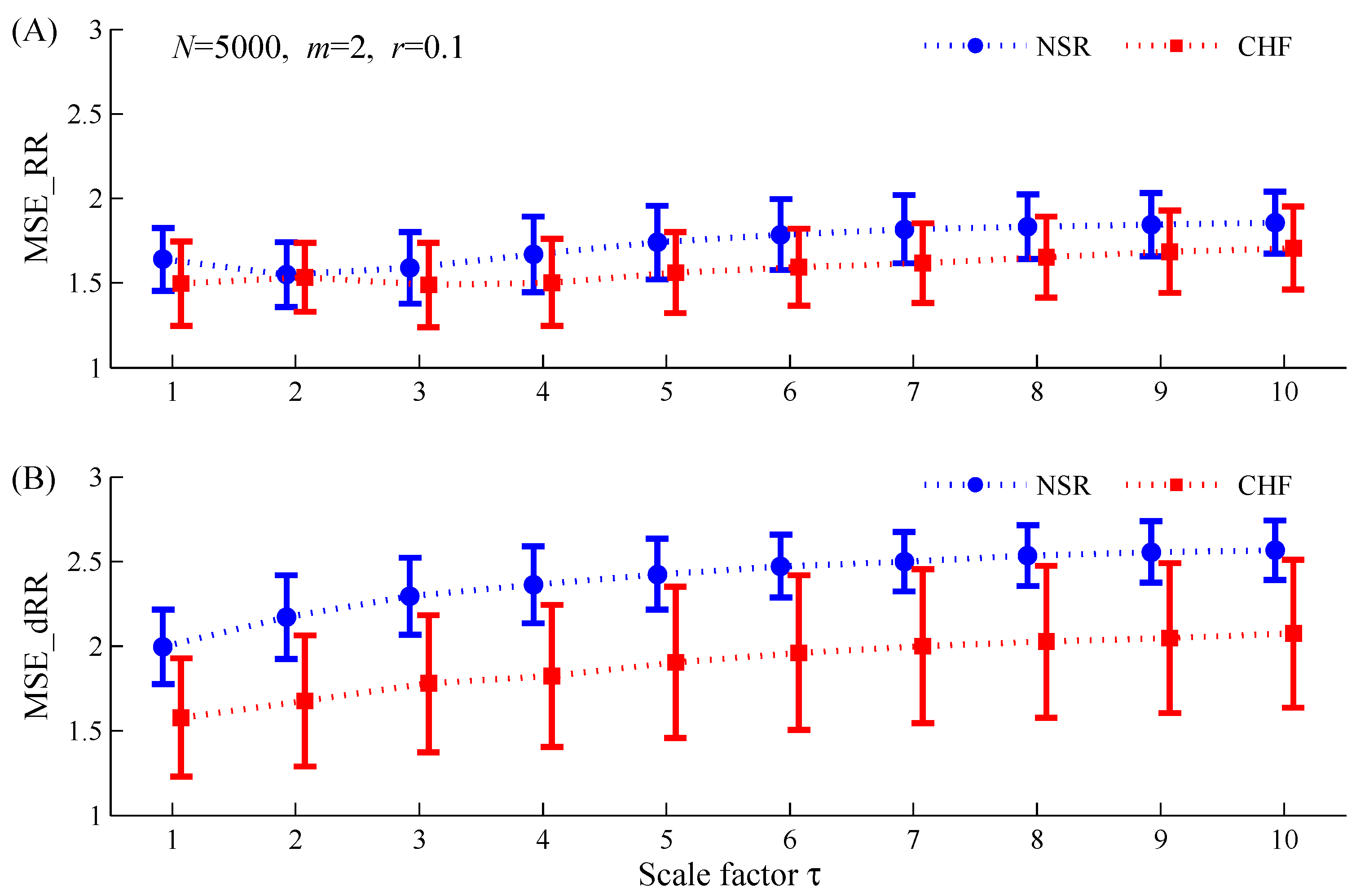
Figure 6.
Dependence of MSE results (mean ± SDs) on the scale factor for the NSR and CHF groups when applied to the time series with length of : (A) MSE_RR results for the original RR interval time series; (B) MSE_dRR results for its difference time series. NSR: normal sinus rhythm group; CHF: congestive heart failure group. The other parameters setting for MSE are: and .

Figure 7.
Examples of ROC curve plots with AUC values for the MSE_RR and MSE_dRR for classifying NSR and CHF groups under four RR segment length types: (A) ; (B) ; (C) ; (D) . Herein, Scale 4 was used.
Figure 7.
Examples of ROC curve plots with AUC values for the MSE_RR and MSE_dRR for classifying NSR and CHF groups under four RR segment length types: (A) ; (B) ; (C) ; (D) . Herein, Scale 4 was used.

Figure 8.
Examples of original RR time series from the CHF patient (chf201). Normal RR intervals are marked as blue circles and the abnormal ones are marked as red circles. The interpolated RR time series are shown in black dots. (a) The original RR time series; (b) the interpolated RR time series.
Figure 8.
Examples of original RR time series from the CHF patient (chf201). Normal RR intervals are marked as blue circles and the abnormal ones are marked as red circles. The interpolated RR time series are shown in black dots. (a) The original RR time series; (b) the interpolated RR time series.

Figure 9.
Dependence of MSE results (mean ± SDs) on the scale factor for the NSR and CHF groups when applied to the RR time series () using two editing methods for the abnormal RR intervals, i.e., the direct deletion method and the interpolation method: (A) MSE_RR results; (B) MSE_dRR results. NSR: normal sinus rhythm group; CHF: congestive heart failure group. The other parameters setting for MSE are: and .


Table 1.
Statistical results of the numbers of RR interval recordings, RR intervals and RR segments from the 54 normal sinus rhythm (NSR) and 29 congestive heart failure (CHF) RR Interval Databases.
Table 1.
Statistical results of the numbers of RR interval recordings, RR intervals and RR segments from the 54 normal sinus rhythm (NSR) and 29 congestive heart failure (CHF) RR Interval Databases.
| Variables | NSR Group | CHF Group |
|---|---|---|
| Name of RR interval recordings | nsr001–nsr054 | chf201–chf229 |
| No. of RR interval recordings | 54 | 29 |
| No. of RR intervals | 5,790,504 | 3,312,195 |
| No. of RR intervals after removing greater than 2 s | 5,780,148 | 3,306,394 |
| No. of RR intervals after removing abnormal heartbeats | 5,738,937 | 3,102,120 |
| No. of RR segments when setting N = 500 | 11,452 | 6192 |
| No. of RR segments when setting N = 1000 | 5711 | 3089 |
| No. of RR segments when setting N = 2000 | 2843 | 1540 |
| No. of RR segments when setting N = 5000 | 1123 | 607 |
Table 2.
Statistical results of Multiscale entropy (MSE) for the NSR and CHF groups by analyzing MSE_RR and MSE_dRR respectively. The RR segment lengths were set as , , and , respectively. Scales 1–10 were used. The other parameters setting for MSE are: and . (The shadows mean there are no significant differences between the two groups).
| Length of RR Segment | Scale Factor | MSE_RR (Original RR Segment) | MSE_dRR (Difference Time Series) | ||||
|---|---|---|---|---|---|---|---|
| NSR | CHF | p-Value | NSR | CHF | p-Value | ||
| 500 | 1 | 1.84 ± 0.16 | 1.53 ± 0.30 | 4 × 10⁻⁸ | 2.00 ± 0.22 | 1.58 ± 0.35 | 1 × 10⁻⁹ |
| 2 | 1.99 ± 0.15 | 1.78 ± 0.27 | 2 × 10⁻⁵ | 2.22 ± 0.26 | 1.69 ± 0.40 | 2 × 10⁻¹⁰ | |
| 3 | 2.04 ± 0.15 | 1.90 ± 0.23 | 9 × 10⁻⁴ | 2.35 ± 0.21 | 1.81 ± 0.42 | 2 × 10⁻¹¹ | |
| 4 | 2.09 ± 0.16 | 1.94 ± 0.22 | 8 × 10⁻⁴ | 2.33 ± 0.14 | 1.85 ± 0.41 | 1 × 10⁻¹¹ | |
| 5 | 2.10 ± 0.13 | 1.97 ± 0.17 | 2 × 10⁻⁴ | 2.29 ± 0.08 | 1.89 ± 0.37 | 3 × 10⁻¹¹ | |
| 6 | 2.03 ± 0.09 | 1.95 ± 0.13 | 9 × 10⁻⁴ | 2.20 ± 0.07 | 1.88 ± 0.33 | 2 × 10⁻⁸ | |
| 7 | 2.11 ± 0.09 | 1.85 ± 0.29 | 7 × 10⁻⁵ | ||||
| 8 | 2.04 ± 0.07 | 1.80 ± 0.26 | 0.003 | ||||
| 9 | 1.76 ± 0.05 | 1.68 ± 0.06 | 5 × 10⁻⁴ | ||||
| 10 | |||||||
| 1000 | 1 | 1.80 ± 0.15 | 1.53 ± 0.29 | 3 × 10⁻⁷ | 2.00 ± 0.22 | 1.58 ± 0.35 | 2 × 10⁻⁹ |
| 2 | 1.86 ± 0.16 | 1.72 ± 0.24 | 0.002 | 2.20 ± 0.25 | 1.68 ± 0.39 | 2 × 10⁻¹⁰ | |
| 3 | 2.34 ± 0.24 | 1.79 ± 0.42 | 9 × 10⁻¹¹ | ||||
| 4 | 1.99 ± 0.18 | 1.85 ± 0.23 | 0.003 | 2.43 ± 0.24 | 1.85 ± 0.45 | 4 × 10⁻¹¹ | |
| 5 | 2.09 ± 0.18 | 1.93 ± 0.23 | 8 × 10⁻⁴ | 2.49 ± 0.21 | 1.92 ± 0.45 | 2 × 10⁻¹¹ | |
| 6 | 2.15 ± 0.17 | 1.97 ± 0.19 | 6 × 10⁻⁵ | 2.50 ± 0.16 | 1.98 ± 0.44 | 1 × 10⁻¹¹ | |
| 7 | 2.18 ± 0.16 | 2.02 ± 0.20 | 1 × 10⁻⁴ | 2.48 ± 0.12 | 2.00 ± 0.43 | 4 × 10⁻¹¹ | |
| 8 | 2.19 ± 0.14 | 2.05 ± 0.17 | 1 × 10⁻⁴ | 2.45 ± 0.09 | 2.03 ± 0.41 | 3 × 10⁻¹⁰ | |
| 9 | 2.17 ± 0.13 | 2.06 ± 0.18 | 0.002 | 2.40 ± 0.08 | 2.03 ± 0.38 | 9 × 10⁻¹⁰ | |
| 10 | 2.32 ± 0.08 | 2.02 ± 0.33 | 7 × 10⁻⁹ | ||||
| 2000 | 1 | 1.75 ± 0.15 | 1.52 ± 0.27 | 4 × 10⁻⁶ | 2.00 ± 0.22 | 1.58 ± 0.35 | 3 × 10⁻⁹ |
| 2 | 2.19 ± 0.25 | 1.68 ± 0.39 | 3 × 10⁻¹⁰ | ||||
| 3 | 2.32 ± 0.24 | 1.78 ± 0.41 | 6 × 10⁻¹¹ | ||||
| 4 | 1.83 ± 0.20 | 1.68 ± 0.25 | 0.003 | 2.39 ± 0.23 | 1.84 ± 0.44 | 6 × 10⁻¹¹ | |
| 5 | 1.92 ± 0.19 | 1.75 ± 0.24 | 8 × 10⁻⁴ | 2.47 ± 0.21 | 1.92 ± 0.47 | 2 × 10⁻¹⁰ | |
| 6 | 1.98 ± 0.19 | 1.79 ± 0.23 | 2 × 10⁻⁴ | 2.53 ± 0.20 | 1.98 ± 0.47 | 1 × 10⁻¹⁰ | |
| 7 | 2.02 ± 0.18 | 1.84 ± 0.23 | 2 × 10⁻⁴ | 2.56 ± 0.19 | 2.02 ± 0.47 | 8 × 10⁻¹¹ | |
| 8 | 2.04 ± 0.18 | 1.88 ± 0.22 | 6 × 10⁻⁴ | 2.59 ± 0.19 | 2.05 ± 0.47 | 1 × 10⁻¹⁰ | |
| 9 | 2.06 ± 0.17 | 1.91 ± 0.22 | 8 × 10⁻⁴ | 2.60 ± 0.18 | 2.08 ± 0.45 | 5 × 10⁻¹¹ | |
| 10 | 2.09 ± 0.17 | 1.94 ± 0.22 | 5 × 10⁻⁴ | 2.59 ± 0.15 | 2.09 ± 0.44 | 4 × 10⁻¹¹ | |
| 5000 | 1 | 1.64 ± 0.19 | 1.50 ± 0.25 | 0.004 | 2.00 ± 0.22 | 1.58 ± 0.35 | 3 × 10⁻⁹ |
| 2 | 2.17 ± 0.25 | 1.68 ± 0.39 | 4 × 10⁻¹⁰ | ||||
| 3 | 2.30 ± 0.23 | 1.78 ± 0.41 | 9 × 10⁻¹¹ | ||||
| 4 | 1.67 ± 0.22 | 1.50 ± 0.26 | 0.003 | 2.36 ± 0.23 | 1.82 ± 0.42 | 4 × 10⁻¹¹ | |
| 5 | 1.74 ± 0.22 | 1.56 ± 0.24 | 0.001 | 2.43 ± 0.21 | 1.90 ± 0.45 | 2 × 10⁻¹⁰ | |
| 6 | 1.79 ± 0.21 | 1.59 ± 0.23 | 2 × 10⁻⁴ | 2.47 ± 0.19 | 1.96 ± 0.46 | 3 × 10⁻¹⁰ | |
| 7 | 1.82 ± 0.20 | 1.62 ± 0.24 | 9 × 10⁻⁵ | 2.50 ± 0.18 | 2.00 ± 0.45 | 3 × 10⁻¹⁰ | |
| 8 | 1.83 ± 0.19 | 1.65 ± 0.24 | 3 × 10⁻⁴ | 2.53 ± 0.18 | 2.03 ± 0.45 | 2 × 10⁻¹⁰ | |
| 9 | 1.84 ± 0.19 | 1.68 ± 0.24 | 0.001 | 2.56 ± 0.18 | 2.05 ± 0.44 | 1 × 10⁻¹⁰ | |
| 10 | 1.86 ± 0.18 | 1.71 ± 0.25 | 0.002 | 2.57 ± 0.17 | 2.07 ± 0.44 | 2 × 10⁻¹⁰ | |
Note: Data are expressed as mean ± standard deviation (SD). NSR: normal sinus rhythm group; CHF: congestive heart failure group.
Table 3.
Results of AUC values (%) for MSE_RR and MSE_dRR for classifying the NSR and CHF groups. Four RR segment length types (,, and ) were evaluated. Scales 1–10 were used. The other parameters setting for MSE are: and .
Table 3.
Results of AUC values (%) for MSE_RR and MSE_dRR for classifying the NSR and CHF groups. Four RR segment length types (,, and ) were evaluated. Scales 1–10 were used. The other parameters setting for MSE are: and .
| Scale Factor | ||||||||
|---|---|---|---|---|---|---|---|---|
| MSE_RR | MSE_dRR | MSE_RR | MSE_dRR | MSE_RR | MSE_dRR | MSE_RR | MSE_dRR | |
| 1 | 79.7 | 82.8 | 78.9 | 82.4 | 77.4 | 82.5 | 69.1 | 82.5 |
| 2 | 75.2 | 84.4 | 67.3 | 84.4 | 61.0 | 83.9 | 52.7 | 83.6 |
| 3 | 69.0 | 84.9 | 64.3 | 84.6 | 62.5 | 84.9 | 64.4 | 84.9 |
| 4 | 70.3 | 82.7 | 68.6 | 84.7 | 68.9 | 84.3 | 68.3 | 85.0 |
| 5 | 71.4 | 84.1 | 71.9 | 85.9 | 71.5 | 83.5 | 69.8 | 83.5 |
| 6 | 70.0 | 80.0 | 74.5 | 83.7 | 73.1 | 82.8 | 71.1 | 82.1 |
| 7 | 63.9 | 80.5 | 71.9 | 83.8 | 72.2 | 83.7 | 72.1 | 81.9 |
| 8 | 55.7 | 80.4 | 71.7 | 81.0 | 69.5 | 83.2 | 69.8 | 82.7 |
| 9 | 84.0 | 73.7 | 66.9 | 79.1 | 69.1 | 83.1 | 66.8 | 83.4 |
| 10 | 46.7 | 61.5 | 61.6 | 81.1 | 70.6 | 83.0 | 66.8 | 81.7 |
| Mean | 68.6 | 79.5 | 69.8 | 83.1 | 69.6 | 83.5 | 67.1 | 83.1 |
| SD | 11.0 | 7.1 | 5.1 | 2.1 | 4.8 | 0.7 | 5.5 | 1.2 |
Table 4.
Results of five-fold cross validation for MSE_RR and MSE_dRR using the default SVM parameter setting. Three RR segment length types (, and ) were evaluated. The other parameters setting for MSE are: and .
Table 4.
Results of five-fold cross validation for MSE_RR and MSE_dRR using the default SVM parameter setting. Three RR segment length types (, and ) were evaluated. The other parameters setting for MSE are: and .
| Length of RR Segment | Fold | MSE_RR (Original RR Segment) | MSE_dRR (Difference Signal) | ||||
|---|---|---|---|---|---|---|---|
| (%) | (%) | (%) | (%) | (%) | (%) | ||
| 1000 | 1 | 71.4 | 66.7 | 68.8 | 80.0 | 90.9 | 87.5 |
| 2 | 80.0 | 75.0 | 76.5 | 100 | 76.9 | 81.3 | |
| 3 | 57.1 | 80.0 | 70.6 | 80.0 | 83.3 | 82.4 | |
| 4 | 66.7 | 81.8 | 76.5 | 80.0 | 91.7 | 88.2 | |
| 5 | 75.0 | 75.0 | 75.0 | 90.9 | 83.3 | 88.2 | |
| Mean | 70.1 | 75.7 | 73.5 | 86.2 | 85.2 | 85.5 | |
| SD | 8.7 | 5.9 | 3.6 | 9.1 | 6.1 | 3.4 | |
| 2000 | 1 | 71.4 | 66.7 | 68.8 | 80.0 | 90.9 | 87.5 |
| 2 | 80.0 | 83.3 | 82.4 | 100 | 84.6 | 87.5 | |
| 3 | 71.4 | 80.0 | 76.5 | 80.0 | 83.3 | 82.4 | |
| 4 | 66.7 | 72.7 | 70.6 | 80.0 | 91.7 | 88.2 | |
| 5 | 75.0 | 83.3 | 81.3 | 81.8 | 83.3 | 82.4 | |
| Mean | 72.9 | 77.2 | 75.9 | 84.4 | 86.8 | 85.6 | |
| SD | 5.0 | 7.3 | 6.1 | 8.8 | 4.2 | 3.0 | |
| 5000 | 1 | 71.4 | 55.6 | 62.5 | 80.0 | 90.9 | 87.5 |
| 2 | 80.0 | 83.3 | 82.4 | 100 | 84.6 | 87.5 | |
| 3 | 71.4 | 80.0 | 76.5 | 80.0 | 83.3 | 82.4 | |
| 4 | 66.7 | 72.7 | 70.6 | 80.0 | 91.7 | 88.2 | |
| 5 | 75.0 | 83.3 | 81.3 | 81.8 | 83.3 | 82.4 | |
| Mean | 72.9 | 75.0 | 74.6 | 84.4 | 86.8 | 85.6 | |
| SD | 5.0 | 11.7 | 8.2 | 8.8 | 4.2 | 3.0 | |
Table 5.
Statistical results of MSE (RR segment length ) for the NSR and CHF groups by analyzing MSE_RR and MSE_dRR respectively. Herein, during the pre-processing for RR interval recording, the abnormal RR intervals were not deleted and were interpolated using the spline interpolation method. Scales 1–10 were used. The other parameters setting for MSE are: and . (The shadows mean there are no significant differences between the two groups).
| Length of RR Segment | Scale Factor | MSE_RR (Original RR Segment) | MSE_dRR (Difference Time Series) | ||||
|---|---|---|---|---|---|---|---|
| NSR | CHF | p-Value | NSR | CHF | p-Value | ||
| 1000 | 1 | 1.79 ± 0.15 | 1.51 ± 0.28 | 4 × 10⁻⁸ | 1.99 ± 0.22 | 1.57 ± 0.34 | 8 × 10⁻¹⁰ |
| 2 | 1.85 ± 0.17 | 1.72 ± 0.24 | 0.005 | 2.19 ± 0.25 | 1.71 ± 0.38 | 9 × 10⁻¹⁰ | |
| 3 | 2.34 ± 0.24 | 1.83 ± 0.42 | 4 × 10⁻¹⁰ | ||||
| 4 | 1.98 ± 0.18 | 1.84 ± 0.23 | 0.003 | 2.42 ± 0.23 | 1.89 ± 0.43 | 1 × 10⁻¹⁰ | |
| 5 | 2.08 ± 0.18 | 1.92 ± 0.24 | 0.001 | 2.48 ± 0.20 | 1.96 ± 0.44 | 2 × 10⁻¹⁰ | |
| 6 | 2.15 ± 0.18 | 1.99 ± 0.22 | 4 × 10⁻⁴ | 2.49 ± 0.15 | 2.01 ± 0.44 | 2 × 10⁻¹⁰ | |
| 7 | 2.18 ± 0.16 | 2.03 ± 0.19 | 4 × 10⁻⁴ | 2.48 ± 0.12 | 2.05 ± 0.41 | 2 × 10⁻¹⁰ | |
| 8 | 2.18 ± 0.14 | 2.06 ± 0.19 | 0.002 | 2.44 ± 0.08 | 2.06 ± 0.38 | 4 × 10⁻¹⁰ | |
| 2.40 ± 0.08 | 2.08 ± 0.36 | 9 × 10⁻⁹ | |||||
| 2.32 ± 0.07 | 2.05 ± 0.33 | 2 × 10⁻⁷ | |||||
Note: Data are expressed as mean ± standard deviation (SD). NSR: normal sinus rhythm group; CHF: congestive heart failure group.
© 2017 by the authors. Licensee MDPI, Basel, Switzerland. This article is an open access article distributed under the terms and conditions of the Creative Commons Attribution (CC BY) license (http://creativecommons.org/licenses/by/4.0/).
Share and Cite
MDPI and ACS Style
Liu, C.; Gao, R. Multiscale Entropy Analysis of the Differential RR Interval Time Series Signal and Its Application in Detecting Congestive Heart Failure. Entropy 2017, 19, 251. https://doi.org/10.3390/e19060251
AMA Style
Liu C, Gao R. Multiscale Entropy Analysis of the Differential RR Interval Time Series Signal and Its Application in Detecting Congestive Heart Failure. Entropy. 2017; 19(6):251. https://doi.org/10.3390/e19060251
Chicago/Turabian StyleLiu, Chengyu, and Rui Gao. 2017. "Multiscale Entropy Analysis of the Differential RR Interval Time Series Signal and Its Application in Detecting Congestive Heart Failure" Entropy 19, no. 6: 251. https://doi.org/10.3390/e19060251
Note that from the first issue of 2016, this journal uses article numbers instead of page numbers. See further details here.