Multiscale Information Theory and the Marginal Utility of Information


1
Department of Mathematics, Emmanuel College, Boston, MA 02115, USA
2
Program for Evolutionary Dynamics, Harvard University, Cambridge, MA 02138, USA
3
Department of Physics, University of Massachusetts-Boston, Boston, MA 02125, USA
4
New England Complex Systems Institute, Cambridge, MA 02139, USA
*
Author to whom correspondence should be addressed.
Entropy 2017, 19(6), 273; https://doi.org/10.3390/e19060273
Submission received: 28 February 2017
/
Revised: 26 May 2017
/
Accepted: 9 June 2017
/
Published: 13 June 2017
(This article belongs to the Special Issue Complexity, Criticality and Computation (C³))
Abstract
:Complex systems display behavior at a range of scales. Large-scale behaviors can emerge from the correlated or dependent behavior of individual small-scale components. To capture this observation in a rigorous and general way, we introduce a formalism for multiscale information theory. Dependent behavior among system components results in overlapping or shared information. A system’s structure is revealed in the sharing of information across the system’s dependencies, each of which has an associated scale. Counting information according to its scale yields the quantity of scale-weighted information, which is conserved when a system is reorganized. In the interest of flexibility we allow information to be quantified using any function that satisfies two basic axioms. Shannon information and vector space dimension are examples. We discuss two quantitative indices that summarize system structure: an existing index, the complexity profile, and a new index, the marginal utility of information. Using simple examples, we show how these indices capture the multiscale structure of complex systems in a quantitative way.
1. Introduction
The field of complex systems seeks to identify, understand and predict common patterns of behavior across the physical, biological and social sciences [1,2,3,4,5,6,7]. It succeeds by tracing these behavior patterns to the structures of the systems in question. We use the term “structure” to mean the totality of quantifiable relationships, or dependencies, among the components comprising a system. Systems from different domains and contexts can share key structural properties, causing them to behave in similar ways. For example, the central limit theorem tells us that the sum over many independent random variables yields an aggregate value whose probability distribution is well-approximated as a Gaussian. This helps us understand systems composed of statistically independent components, whether those components are molecules, microbes or human beings. Likewise, different chemical elements and compounds display essentially the same behavior near their respective critical points. The critical exponents which encapsulate the thermodynamic properties of a substance are the same for all substances in the same universality class, and membership in a universality class depends upon structural features such as dimensionality and symmetry properties, rather than on details of chemical composition [8].
Outside of known universality classes, identifying the key structural features that dictate the behavior of a system or class of systems often relies upon an ad hoc leap of intuition. This becomes particularly challenging for complex systems, where the set of system components is not only large, but also interwoven and resistant to decomposition. Information theory [9,10] holds promise as a general tool for quantifying the dependencies that comprise a system’s structure [11]. We can consider the amount of information that would be obtained from observations of any component or set of components. Dependencies mean that one observation can be fully or partially inferred from another, thereby reducing the amount of joint information present in a set of components, compared to the amount that would be present without those dependencies. Information theory allows one to quantify not only fixed or rigid relationships among components, but also “soft” relationships that are not fully determinate, e.g., statistical or probabilistic relationships.
However, traditional information theory is primarily concerned with amounts of independent bits of information. Consequently, each bit of non-redundant information is regarded as equally significant, and redundant information is typically considered irrelevant, except insofar as it provides error correction [10,12]. These features of information theory are natural in applications to communication, but present a limitation when characterizing the structure of a physical, biological, or social system. In a system of celestial bodies, the same amount of information might describe the position of a moon, a planet, or a star. Likewise, the same amount of information might describe the velocity of a solitary grasshopper, or the mean velocity of a locust swarm. A purely information-theoretic treatment has no mechanism to represent the fact that these observables, despite containing the same amount of information, differ greatly in their significance.
Overcoming this limitation requires a multiscale approach to information theory [13,14,15,16,17,18]—one that identifies not only the amount of information in a given observable but also its scale, defined as the number or volume of components to which it applies. Information describing a star’s position applies at a much larger scale than information describing a moon’s position. In shifting from traditional information theory to a multiscale approach, redundant information becomes not irrelevant but crucial: Redundancy among smaller-scale behaviors gives rise to larger-scale behaviors. In a locust swarm, measurements of individual velocity are highly redundant, in that the velocity of all individuals can be inferred with reasonable accuracy by measuring the velocity of just one individual. The multiscale approach, rather than collapsing this redundant information into a raw number of independent bits, identifies this information as large-scale and significant precisely because it is redundant across many individuals.
The multiscale approach to information theory also sheds light on a classic difficulty in the field of complex systems: to clarify what a “complex system” actually is. Naïvely, one might think to define complex systems as those that display the highest complexity, as quantified using Shannon information or other standard measures. However, the systems deemed the most “complex” by these measures are those in which the components behave independently of each other, such as ideal gases. Such systems lack the multiscale regularities and interdependencies that characterize the systems typically studied by complex systems researchers. Some theorists have argued that true complexity is best viewed as occupying a position between order and randomness [19,20,21]. Music is, so the argument goes, intermediate between still air and white noise. But although complex systems contain both order and randomness, they do not appear to be mere blends of the two. A more satisfying answer is that complex systems display behavior across a wide range of scales. For example, stock markets can exhibit small-scale behavior, as when an individual investor sells a small number of shares for reasons unrelated to overall market activity. They can also exhibit large-scale behavior, e.g., a large institutional investor sells many shares [22], or many individual investors sell shares simultaneously in a market panic [23].
Formalizing these ideas requires a synthesis of statistical physics and information theory. Statistical physics [24,25,26,27]—in particular the renormalization group of phase transitions [28,29]—provides a notion of scale in which individual components acting in concert can be considered equivalent to larger-scale units. Information theory provides the tool of multivariate mutual information: the information shared among an arbitrary number of variables (also called interaction information or co-information) [13,14,15,16,17,30,31,32,33,34,35,36,37,38,39]. These threads were combined in the complexity profile [13,14,15,16,17,18], a quantitative index of structure that characterizes the amount of information applying at a given scale or higher. In the context of the complexity profile, the multivariate mutual information of a set of n variables is considered to have scale n. In this way, information is understood to have scale equal to the multiplicity (or redundancy) at which it arises—an idea which is also implicit in other works on multivariate mutual information [40,41].
Here we present a mathematical formalism for multiscale information theory, for use in quantifying the structure of complex systems. Our starting point is the idea discussed in the previous paragraph, that information has scale equal to the multiplicity at which it arises. We formalize this idea mathematically and generalize it in two directions: First, we allow each system component to have an arbitrary intrinsic scale, reflecting its inherent size, volume, or multiplicity. For example, the mammalian muscular system includes both large and small muscles, corresponding to different scales of environmental challenge (e.g., pursuing prey and escaping from predators versus chewing food) [42]. Scales are additive in our formalism, in the sense that a set of components acting in perfect coordination is formally equivalent to a single component with scale equal to the sum of the scales of the individual components. This equivalence can greatly simplify the representation of a system. Consider, for example, an avalanche consisting of differently-sized rocks. To represent this avalanche within the framework of traditional (single-scale) information theory, one must either neglect the differences in size (thereby diminishing the utility of the representation) or else model each rock by a collection of myriad statistical variables, each corresponding to a equally-sized portion. Our formalism, by incorporating scale as a fundamental quantity, allows each rock to be represented in a direct and physically meaningful way.
Second, in the interest of generality, we use a new axiomatized definition of information, which encompasses traditional measures such as Shannon information as well as other quantifications of freedom or indeterminacy. In this way, our formalism is applicable to system representations for which traditional information measures cannot be used.
Using these concepts of information and scale, we identify how a system’s joint information is distributed across each of its irreducible dependencies—relationships among some components conditional on all others. Each irreducible dependency has an associated scale, equal to the sum of the scales of the components included in this dependency. This formalizes the idea that any information pertaining to a system applies at a particular scale or combination of scales. Multiplying quantities of information by the scales at which they apply yields the scale-weighted information, a quantity that is conserved when a system is reorganized or restructured.
We use this multiscale formalism to develop quantitative indices that summarize important aspects of a system’s structure. We generalize the complexity profile to allow for arbitrary intrinsic scales and a variety of information measures. We also introduce a new index, the marginal utility of information (MUI), which characterizes the extent to which a system can be described using limited amounts of information. The complexity profile and the MUI both capture a tradeoff of complexity versus scale that is present in all systems.
Our basic definitions of information, scale, and systems are presented in Section 2, Section 3 and Section 4, respectively. Section 5 formalizes the multiscale approach to information theory by defining the information and scale of each of a system’s dependencies. Section 6 and Section 7 discuss our two indices of structure. Section 8 establishes a mathematical relationship between these two indices for a special class of systems. Section 9 applies our indices of structure to the noisy voter model [43]. We conclude in Section 10 and Section 11 by discussing connections between our formalism and other work in information theory and complex systems science.
2. Information
We begin by introducing a generalized, axiomatic notion of information. Conceptually, information specifies a particular entity out of a set of possibilities and thus enables us to describe or characterize that entity. Information measures such as Shannon information quantify the amount of resources needed in this specification. Rather than adopting a specific information measure, we consider that the amount of information may be quantified in different ways, each appropriate to different contexts.
Let A be the set of components in a system. An information function, H, assigns a nonnegative real number to each subset , representing the amount of information needed to describe the components in U. (Throughout, the subset notation includes the possibility that .) We require that an information function satisfy two axioms:
- Monotonicity: The information in a subset U that is contained in a subset V cannot have more information than V, that is, .
- Strong subadditivity: Given two subsets, the information contained in both cannot exceed the information in each of them separately minus the information in their intersection:
Strong subadditvity expresses how information combines when parts of a system (U and V) are regarded as a whole (). Information regarding U may overlap with information regarding V for two reasons. First, U and V may share components; this is corrected for by subtracting . Second, constraints in the behavior of non-shared components may reduce the information needed to describe the whole. Thus, information describing the whole may be reduced due to overlaps or redundancies in the information applying to different parts, but it cannot be increased.
In contrast to other axiomatizations of information, which uniquely specify the Shannon information [9,44,45,46] or a particular family of measures [47,48,49,50], the two axioms above are compatible with a variety of different measures that quantify information or complexity:
- Microcanonical or Hartley entropy: For a system with a finite number of joint states, is an information function, where m is the number of joint states available to the subset U of components. Here, information content measures the number of yes-or-no questions which must be answered to identify one joint state out of m possibilities.
- Shannon entropy: For a system characterized by a probability distribution over all possible joint states, is an information function, where are the probabilities of the joint states available to the components in U [9]. Here, information content measures the number of yes-or-no questions which must be answered to identify one joint state out of all the joint states available to U, where more probable states can be identified more concisely.
- Tsallis entropy: The Tsallis entropy [51,52] is a generalization of the Shannon entropy with applications to nonextensive statistical mechanics. For the same setting as in Shannon entropy, Tsallis entropy is defined as for some parameter . Shannon entropy is recovered in the limit . Tsallis entropy is an information function for (but not for ); this follows from Proposition 2.1 and Theorem 3.4 of [53].
- Logarithm of period: For a deterministic dynamic system with periodic behavior, an information function can be defined as the logarithm of the period of a set U of components (i.e., the time it takes for the joint state of these components to return to an initial joint state) [54]. This information function measures the number of questions which one should expect to answer in order to locate the position of those components in their cycle.
- Vector space dimension: Consider a system of n components, each of whose state is described by a real number. Then the joint states of any subset U of components can be described by points in some linear subspace of . The minimal dimension of such a subspace is an information function, equal to the number of coordinates one must specify in order to identify the joint state of U.
- Matroid rank: A matroid consists of a set of elements called the ground set, together with a rank function that takes values on subsets of the ground set. Rank functions are defined to include the monotonicity and strong subadditivity properties [55], and generalize the notion of vector subspace dimension. Consequently, the rank function of a matroid is an information function, with the ground set identified as the set of system components.
In principle, measurements of algorithmic complexity may also be regarded as information functions. For example, when a subset U can be encoded as a binary string, the algorithmic complexity can be quantified as the length of the shortest self-delimiting program producing this string, with respect to some universal Turing machine [56]. Information content then measures the number of machine-language instructions which must be given to reconstruct U. Algorithmic complexity—at least under certain formulations—obeys versions of the monotonicity and strong subadditivity axioms [56,57]. However, while conceptually clean, this definition is difficult to apply quantitatively. First, the algorithmic complexity is only defined up to a constant which depends on the choice of universal Turing machine. Second, as a consequence of the halting problem, algorithmic complexity can only be bounded, not computed exactly.
3. Scale
A defining feature of complex systems is that they exhibit nontrivial behavior on multiple scales [1,13,14]. While the term “scale” has different meanings in different scientific contexts, we use the term scale here in the sense of the number of entities or units acting in concert, with each involved entity potentially weighted according to a measure of importance.
For many systems, it is reasonable to regard all components as having a priori equal scale. In this case we may choose the units of scale so that each component has scale equal to 1. This convention was used in previous work on the complexity profile [13,14,15,16,17]. However, it is in many cases necessary to represent the components of a system as having different intrinsic scales, reflecting their built-in size, multiplicity or redundancy. For example, in a system of many physical bodies, it may be natural to identify the scale of each body as a function of its mass, reflecting the fact that each body comprises many molecules moving in concert. In a system of investment banks [58,59,60], it may be desirable to assign weight to each bank according to its volume of assets. In these cases, we denote the a priori scale of a system component a by a positive real number , defined in terms of some meaningful scale unit.
Scales are additive, in the sense that a set of completely interdependent components can be replaced by a single component whose scale is equal to the sum of the scales of the individual components. We describe this property formally in Section 5.4 and in Appendix B.
4. Systems
We formally define a system to comprise three elements:
- A finite set A of components,
- An information function , giving the information in each subset ,
- A scale function , giving the intrinsic scale of each compoent .
The choice of information and scale functions will reflect how the system is modeled mathematically, and the kind of statements we can make about its structure. We omit the subscripts from H and when only one system is under consideration.
In this work, we treat the three elements of a system as unchanging, even though the system itself may be dynamic (existing in a sequence of states through time). A dynamic system can be represented as a set of time histories, or—using the approach of ergodic theory—by defining a probability distribution over states with probabilities corresponding to frequencies of occupancy over extended periods of time. The methods outlined here could also be used to explore the dynamics or histories of a system’s structure, using information and scale functions whose values vary as relationships change within a system over time. However, our current work focuses only on the static or time-averaged properties of a system.
In requiring that the set A of components be finite, we exclude, for example, systems represented as continuum fields, in which each point in a continuous space might be regarded as a component. While the concepts of multiscale information theory may still be useful in thinking about such systems, the mathematical representation of these concepts presents challenges that are beyond the scope of this work.
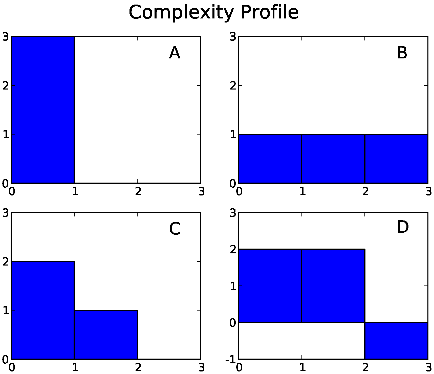
We shall use four simple systems as running examples. Each consists of three binary random variables, each having intrinsic scale one.
- Example A: Three independent components. Each component is equally likely to be in state 0 or state 1, and the system as a whole is equally likely to be in any of its eight possible states.
- Example B: Three completely interdependent components. Each component is equally likely to be in state 0 or state 1, but all three components are always in the same state.
- Example C: Independent blocks of dependent components. Each component is equally likely to take the value 0 or 1; however, the first two components always take the same value, while the third can take either value independently of the coupled pair.
- Example D: The parity bit system. The components can exist in the states 110, 101, 011, or 000 with equal probability. In each state, each component is equal to the parity (0 if even; 1 if odd) of the sum of the other two. Any two of the component are statistically independent of each other, but the three as a whole are constrained to have an even sum.
We define a subsystem of as a triple , where B is a subset of A, is the restriction of to subsets of B, and is the restriction of to elements of B.
5. Multiscale Information Theory
Here we formalize the multiscale approach to information theory. We begin by introducing notation for dependencies. We then identify how information is shared across irreducible dependencies, generalizing the notion of multivariate mutual information [13,14,15,16,17,30,31,32,33,34,35,36,37,38,39] to an arbitrary information function. We then define the scale of a dependency and introduce the quantity of scale-weighted information. Finally, we formalize the key concepts of independence and complete interdependence.
5.1. Dependencies
A dependency among a collection of components is the relationship (if any) among these components such that the behavior of some of the components is in part obtainable from the behavior of others. We denote this dependency by the expression . This expression represents a relationship, rather than a number or quantity. We use a semicolon to keep our notation consistent with information theory (in particular, with multivariate mutual information; see Section 5.2).
We can identify a more general concept of conditional dependencies. Consider two disjoint sets of components and . The conditional dependency represents the relationship (if any) between such that the behavior of some of these components can yield improved inferences about the behavior of others, relative to what could be inferred from the behavior of . We call this the dependency of given , and we say are included in this dependency, while are excluded.
We call a dependency irreducible if every system component is either included or excluded. We denote the set of all irreducible dependencies of a system by . A system’s dependencies can be organized in a Venn diagram, which we call a dependency diagram (Figure 1).
The relationship between the components and dependencies of can be captured by a mapping, which we denote by , from A to subsets of . A component maps to the set of irreducible dependencies that include a (or in visual terms, the region of the dependency diagram that corresponds to component a). For example, in a system of three components a, b, c, we have
We extend the domain of to subsets of components, by mapping each subset onto to the set of all irreducible dependencies that include at least one element of U; for example,
Visually, is the union of the circles representing a and b in the dependency diagram. Finally, we extend the domain of to dependencies, by mapping the dependency onto the set of all irreducible dependencies that include and exclude ; for example,
Visually, consists of the regions corresponding to a but not to c.
5.2. Information Quantity in Dependencies
Here we define the shared information, , of a dependency x in a system . I generalizes the multivariate mutual information [13,14,15,16,17,30,31,32,33,34,35,36,37,38,39] to an arbitrary information function H. We note that H and I characterize the same quantity—information—but are applied to different kinds of arguments: H is applied to subsets of components of , while I is applied to dependencies.
The values of I on irreducible dependencies x of are uniquely determined by the system of equations
As U runs over all subsets of A, the resulting system of equations determines the values , , in terms of the values , . The solution is an instance of the inclusion-exclusion principle [61], and can also be obtained by Gaussian elimination. An explicit formula obtained in the context of Shannon information [32] applies as well to any information function. Figure 2 shows the information in each irreducible dependecy for our four running examples.
We extend I to dependencies that are not irreducible by defining the shared information to be equal to the sum of the values of for all irreducible dependencies y encompassed by a dependency x:
Our notation corresponds to that of Shannon information theory. For example, in a system of two components a and b, solving (5) yields
Above, is shorthand for ; we use similar shorthand throughout. Equation (7) coincides with the classical definition of mutual information [9,10], with H representing joint Shannon information. Similarly, is the conditional entropy of given , and is the conditional mutual information of and given . For a dependency including more than two components, is the multivariate mutual information (also called interaction information or co-information) of the dependency x [30,31,32,33,36,37,38,39].
For any information function H, we observe that the information of one component conditioned on others, the conditional information is nonnegative due to the monotonicity axiom. Likewise, the mutual information of two components conditioned on others, , is nonnegative due to the strong subadditivity axiom. However, the information shared among three or more components can be negative. This is illustrated in running Example D, for which the tertiary shared information is negative (Figure 2D). Such negative values appear to capture an important property of dependencies, but their interpretation is the subject of continuing discussion [34,36,37,62,63].
5.3. Scale-Weighted Information
Multiscale information theory is based on the principle that any information about a system should be understood as applying at a specific scale. Information shared among a set of components—arising from dependent behavior among these components—has scale equal to the sum of the scales of these components. This principle was first discussed in the context of the complexity profile [13,14,15,16,17], and is also implicit in other works on multivariate information theory [40,41], as we discuss in Section 10.2.
To formalize this principle, we define the scale of an irreducible dependency to be equal to the total scale of all components included in x:
The information in an irreducible dependency is understood to apply at scale . Large-scale information pertains to many components and/or to components of large intrinsic scale; whereas small-scale information pertains to few components, and/or components of small intrinsic scale. In running Example C (Figure 2C), the bit of information that applies to components a and c has scale 2, while the bit applying to component b has scale 1.
The overall significance of a dependency in a system depends on both its information and its scale. It therefore natural to weight quantities of information by their scale. We define the scale-weighted information of an irreducible dependency x to be the scale of x times its information quantity
Extending this definition, we define the scale-weighted information of any subset of the dependence space to be the sum of the scale-weighted information of each irreducible-dependency in this subset:
The scale-weighted information of the entire dependency space —that is, the scale-weighted information of the system —is equal to the sum of the scale-weighted information of each component:
As we show in Appendix A, this property arises directly from the fact that scale-weighted information counts redundant information according to its multiplicity or total scale.
According to Equation (11), the total scale-weighted information does not change if the system is reorganized or restructured, as long as the information and scale of each individual component is maintained. The value can therefore be considered a conserved quantity. The existence of this conserved quantity implies a tradeoff of information versus scale, which can be illustrated using the example of a stock market. If investors act largely independently of each other, information overlaps are minimal. The total amount of information is large, but most of this information is small-scale—applying only to a single investor at a time. On the other hand, in a market panic, there is much overlapping or redundant information in their actions—the behavior of one can be largely inferred from the behavior of others [23]. Because of this redundancy, the amount of information needed to describe their collective behavior is low. This redundancy also makes this collective behavior large-scale and highly significant.
5.4. Independence and Complete Interdependence
Components are independent if their joint information is equal to the sum of the information in each separately:
In running Example C, components a, b, and c are independent. This definition generalizes standard notions of independence in information theory, linear algebra, and matroid theory.
We extend the notion of independence to subsystems: subsystems of , for , are defined to be independent of one another if
We recall from Section 4 that is the restriction of to subsets of . In running Example C, the subsystem comprised of components a and c is independent of the subsystem comprised of component b.
Independence has the following hereditary property [64]: if subsystems are independent, then all components and subsystems of are independent of all components and subsystems of , for all . We prove the hereditary property of independence from our axioms in Appendix C.
At the opposite extreme, we define a set of components to be completely interdependent if for any component . In words, any information applying to any component in U applies to all components in U.
A set of completely interdependent components can be replaced by a single component of scale to obtain an equivalent, reduced representation of the system. Thus, in running Example C, the set is completely interdependent, and can be replaced by a single component of scale two. We show in Appendix B that replacements of this kind preserve all relevant quantities of information and scale.
6. Complexity Profile
We now turn to quantitative indices that summarize a system’s structure. One such index is the complexity profile [13,14,15,16,17], which concretizes the observation that a complex system exhibits structure at multiple scales. We define the complexity profile of a system to be a real-valued function of a positive real number y, equal to the total amount of information at scale y or higher in :
Equation (14) generalizes previous definitions of the complexity profile [13,14,15,16,17], which use Shannon information as the information function and consider all components to have scale one.
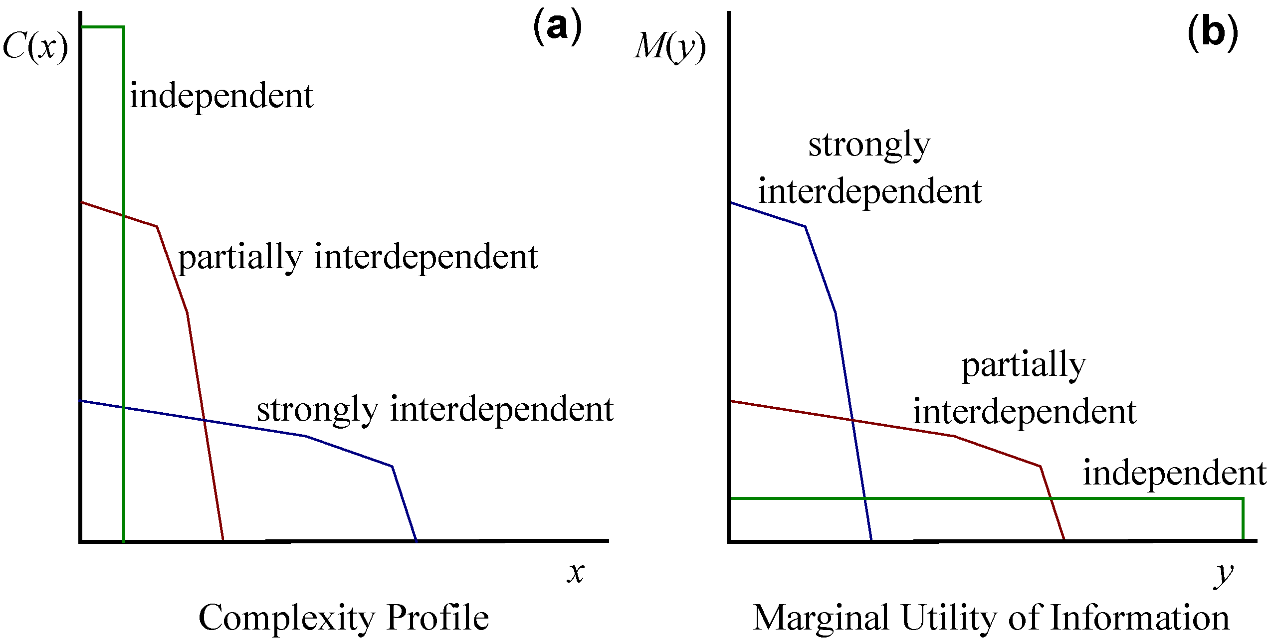
The complexity profile reveals the levels of interdependence in a system. For systems where components are highly independent, is large and decreases sharply in y, since only small amounts of information apply at large scales in such a system. Conversely, in rigid or strongly interdependent systems, is small and the decrease in is shallower, reflecting the prevalence of large-scale information, as shown in in Figure 3. We plot the complexity profiles of our four running examples in Figure 4.
Previous works have developed and applied an explicit formula for the complexity profile [13,14,16,17,35] for cases where all components have equal intrinsic scales, for all . To construct this formula, we first define the quantity as the sum of the joint information of all collections of j components:
The complexity profile can then be expressed as
where is the number of components in [13,14]. The coefficients in this formula can be inferred from the inclusion-exclusion principle [61]; see [13] for a derivation.
The complexity profile has the following properties:
- Conservation law: The area under is equal to the total scale-weighted information of the system, and is therefore independent of the way the components depend on each other [13]:This result follows from the conservation law for scale-weighted information, Equation (11), as shown in Appendix A.
- Total system information: At the lowest scale , corresponds to the overall joint information: . For physical systems with the Shannon information function, this is the total entropy of the system, in units of information rather than the usual thermodynamic units.
- Additivity: If a system is the union of two independent subsystems and , the complexity profile of the full system is the sum of the profiles for the two subsystems, . We prove this property Appendix D.
Due to the combinatorial number of dependencies for an arbitrary system, calculation of the complexity profile may be computationally prohibitive; however, computationally tractable approximations to the complexity profile have been developed [15].
The complexity profile has connections to a number of other information-theoretic characterizations of structure and dependencies among sets of random variables [38,40,41,65,66,67], as we discuss in Section 10.2. What distinguishes the complexity profile from these other approaches is the explicit inclusion of scale as an axis complementary to information.
7. Marginal Utility of Information
Here we introduce an new index characterizing multiscale structure: the marginal utility of information (MUI), denoted . The MUI quantifies how well a system can be characterized using a limited amount of information.
To obtain this index, we first ask how much scale-weighted information (as defined in Section 5.3) can be represented using y or fewer units of information. We call this quantity the maximal utility of information, denoted . For small values of y, an optimal characterization will convey only large-scale features of the system. As y increases, smaller-scale features will be progressively included. For a given system , the maximal amount of scale-weighted information that can be represented, , is constrained not only by the information limit y, but also by the pattern of information overlaps in —that is, the structure of . More strongly interdependent systems allow for larger amounts of scale-weighted information to be described using the same amount of information y.
We define the marginal utility of information as the derivative of maximal utility: . quantifies how much scale-weighted information each additional unit of information can impart. The value of , being the derivative of scale-weighted information with respect to information, has units of scale. declines steeply for rigid or strongly interdependent systems, and shallowly for weakly interdependent systems.
We now develop the formal definition of . We call any entity d that imparts information about system a descriptor of . The utility of a descriptor will be defined as a quantity of the form
For this to be a meaningful expression, we consider each descriptor d to be an element of an augmented system , whose components include d as well as the original components of , which is a subsystem of . The amount of information that d conveys about any subset of components is given by
For example, the amount that d conveys about a component can be written . is the total information d imparts about the system. Because the original system is a subsystem of , the augmented information function coincides with on subsets of A.
The quantities are constrained by the structure of and the axioms of information functions. Applying these axioms, we arrive at the following constraints on :
- (i)
- for all subsets .
- (ii)
- For any pair of nested subsets , .
- (iii)
- For any pair of subsets ,
To obtain the maximum utility of information, we interpret the values as variables subject to the above constraints. We define as the maximum value of the utility expression, Equation (18), as vary subject to constraints (i)–(iii) and that the total information d imparts about is less than or equal to y: .
characterizes the maximal amount of scale-weighted information that could in principle be conveyed about using y or less units of information, taking into account the information-sharing in and the fundamental constraints on how information can be shared. is well-defined since it is the maximal value of a linear function on a bounded set. Moreover, elementary results in linear programming theory [68] imply that is piecewise linear, increasing and concave in y.
The above results imply that the marginal utility of information, , is piecewise constant, positive and nonincreasing. The MUI thus avoids the issue of counterintuitive negative values. The value of can be understood as the additional scale units that can be described by an additional bit of information, given that the first y bits have been optimally utilized. Code for computing the MUI has been developed and is available online [69].
The marginal utility of information has the following additional properties:
- 1.
- Conservation law: The total area under the curve equals the total scale-weighted information of the system:This property follows from the observation that, since is the derivative of , the area under this curve is equal to the maximal utility of any descriptor, which is equal to since utility is defined in terms of scale-weighted information.
- 2.
- Total system information: The marginal utility vanishes for information values larger than the total system information, for , since, for higher values, the system has already been fully described.
- 3.
- Additivity: If separates into independent subsystems and , thenThe proof follows from recognizing that, since information can apply either to or to but not both, an optimal description allots some amount of information to subsystem , and the rest, , to subsystem . The optimum is achieved when the total maximal utility over these two subsystems is maximized. Taking the derivative of both sides and invoking the concavity of U yields a corresponding formula for the marginal utility M:Equations (21) and (22) are proven in Appendix E. This additivity property can also be expressed as the reflection (generalized inverse) of M. For any piecewise-constant, nonincreasing function f, we define the reflection asA generalized inverse [15] is needed since, for piecewise constant functions, there exist x-values for which there is no y such that . For such values, is the largest y such that does not exceed x. This operation is a reflection about the line , and applying it twice recovers the original function. If comprises independent subsystems and , the additivity property, Equation (22), can be written in terms of the reflection asEquation (24) is proven in Appendix E.
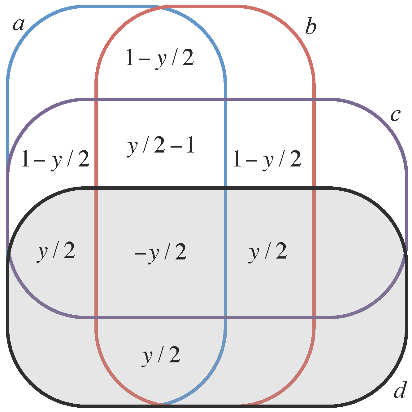
Plots of the MUI for our four running examples are shown in Figure 5. The most interesting case is the parity bit system, Example D, for which the marginal utility is
The optimal description scheme leading to this marginal utility is shown in Figure 6. The marginal utility of information captures the intermediate level of interdependency among components in Example D, in contrast to the maximal independence and maximal interdependence in Examples A and B, respectively (Figure 5). For an N-component generalization of Example D, in which each component acts as a parity bit for all others, we show in Appendix F that the MUI is given by
The MUI is similar in spirit to, and can be approximated by, principal components analysis, Information Bottleneck methods [70,71,72,73], and other methods that characterize the best possible description of a system using limited resources [66,74,75,76,77,78,79]. We discuss these connections in Section 10.3.
8. Reflection Principle for Systems of Independent Blocks
For systems with a particularly simple structure, the complexity profile and the MUI turn out to be reflections (generalized inverses) of each other. The simplest case is a system consisting of a single component a. In this case, according to Equation (14), the complexity profile has value for and zero for :
Above, is a step function with value 1 for and 0 otherwise. To compute the marginal utility of information for this system, we observe that a descriptor with maximal utility has for each value of the informational constraint y, and it follows that
We observe that and are reflections of each other: , where is defined in Equation (23).
We next consider a system whose components are all independent of each other. Additivity over independent subsystems (Property 3 in Section 6 and Section 7), together with Equations (27) and (28), implies
Thus the reflection principle holds for systems of independent components.
More generally, one can consider a system of “independent blocks”—that is, a system that can be partitioned into independent subsystems, where the components of each subsystem are completely interdependent (see Section 5.4 for definitions.) Running example C is such a system, in that it can be partitioned into independent subsystems with component sets and , and each of these sets is completely interdependent. We show in Appendix B that any set of completely interdependent components can be replaced by a single component, with scale equal to the sum of the scales of the replaced components, without altering the complexity profile or MUI. Thus, for systems of independent blocks, each block can be collapsed into a single component, whereupon Equation (29) applies and the reflection principle holds.
We have thus established that for any system of independent blocks, the complexity profile and the MUI are reflections of each other . However, this relationship does not hold for every system. and are not reflections of each other in the case of Example D, and, more generally, for a class of systems that exhibit negative information, as shown in Equation (26).
9. Application to Noisy Voter Model
As an application of our framework, we compute the marginal utility of information for the noisy voter model [43] on a complete graph. This model is a stochastic process with N “voters”. Each voter, , can exist in one of two states, which we label . Each voter updates its state at Poisson rate 1. With probability u it chooses with equal probability; otherwise, with probability , it copies a random other individual. Here is noise (or mutation) parameter that mediates the level of interdependence among voters. It follows that voter i flips its state (from to or vice versa) at Poisson rate
For , voters are typically in consensus; for , all voters behave independently. The noisy voter model is mathematically equivalent to the Moran model [80] of neutral drift with mutation, and to a model of financial behavior on networks [23,81].
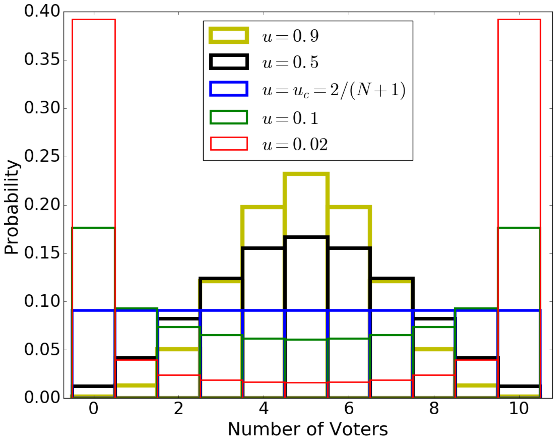
This model has a stationary distribution in which the number m of voters in the state has a beta-binomial distribution (Figure 7) [18,82]:
For small u, P is concentrated on the “consensus” states 0 and N, converging to the uniform distribution on these states as . For large u, P exhibits a central tendency around , and converges to the binomial distribution with as . These two modes are separated by the critical value of , at which and P becomes the uniform distribution on . This is the scenario in which mutation exactly balances the uniformizing effect of faithful copying. As , P converges to the uniform distribution on the states 0 and N.
The noisy voter model on a complete graph possesses exchange symmetry, meaning its behavior is preserved under permutation of its components. As a consequence, if subsets U and V have the same cardinality, , then they have the same information, . The information function is therefore fully characterized by the quantities , where is the information in each subset with components.
To calculate the MUI for systems with exchange symmetry, it suffices to consider descriptors that also possess exchange symmetry, so that whenever . Denoting by the information that a descriptor imparts about a subset of size n, constraints (i)–(iii) of Section 7 reduce to
- (i)
- for all ,
- (ii)
- for all ,
- (iii)
- for all .
The maximum utility of information is the maximum value of , subject to (i)–(iii) above and . Since the number of constraints is polynomial in N, the maximum utility—and therefore the MUI—are readily computable.
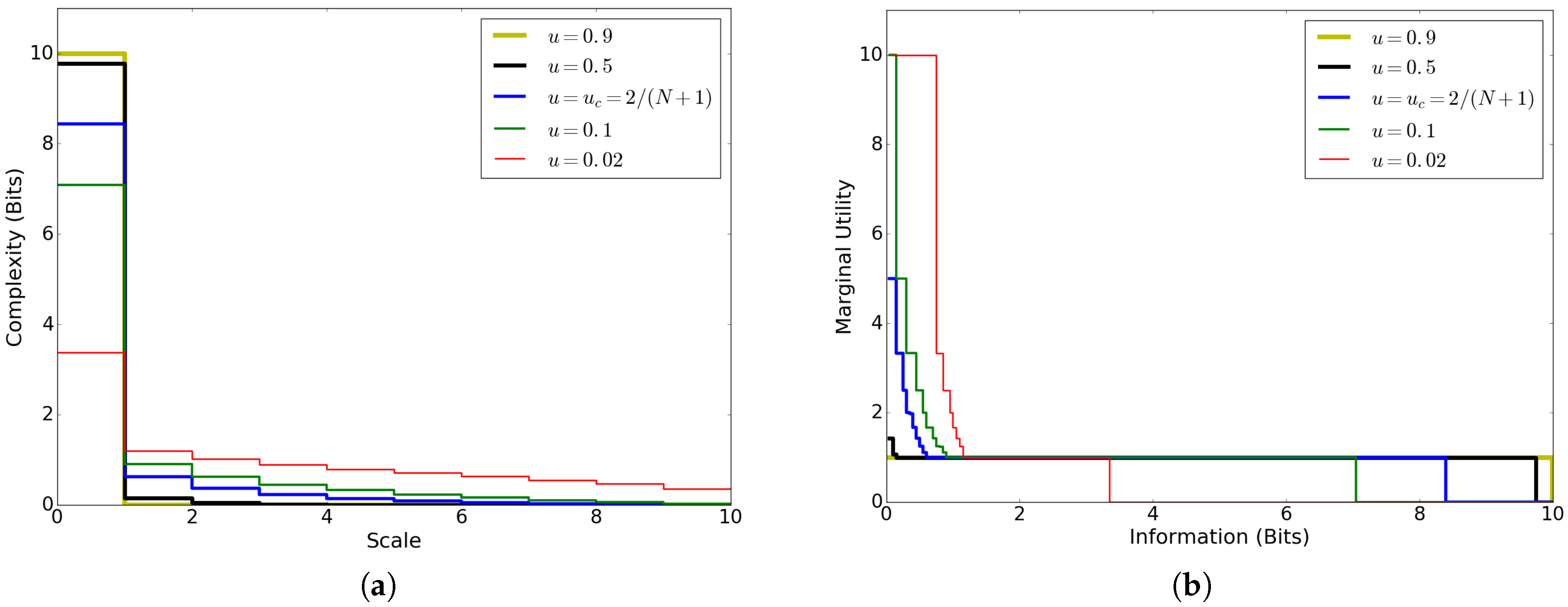
The complexity profile and MUI for this model (Figure 8) both capture how the interdependence of voters is mediated by the noise parameter u. For small u, conformity among voters leads to large-scale information (positive for large x) and enables efficient partial descriptions of the system (large for small y). For large u, weak dependence among voters means that most information applies at small scale ( decreases rapidly) and optimal descriptions cannot do much better than to describe each component singly ( for most values of y). Unlike the case of independent block systems (Section 8), the complexity profile and MUI are not reflections of each other for this model, but the reflection of each is qualitatively similar to the other.
10. Discussion
10.1. Potential Applications
Here we have presented a multiscale extension of information theory, along with two quantitative indices, as tools the analysis of structure in complex systems. Our generalized, axiomatic definition of information enables this framework to be applied to a variety of physical, biological, social, and economic systems. In particular, we envision applications to spin systems [1,17,83,84], gene regulatory systems [85,86,87,88,89,90,91], neural systems [92,93,94], biological swarming [95,96,97], spatial evolutionary dynamics [82,98,99], and financial markets [22,59,81,100,101,102,103,104,105].
In each of these systems, multiscale information theory enables the analysis of such questions as: Do components (genes, neurons, investors, etc.) behave largely independently, or are their behaviors strongly interdependent? How significant are intermediate scales of organization such as the genetic pathway, the cerebral lobe, or the financial sector? Can other “hidden” scales of organization be identified? Do the scales of behavior vary across different instances of a particular kind of system (e.g., gene regulation in stem versus differentiated cells; neural systems across taxa)? And how do the scales of organization in these systems compare to the scales of challenges they face?
The realization of these applications faces a computational hurdle: a full characterization of a system’s structure requires the computation of informational quantities. Thus for large real-world systems, efficient approximations must be developed. Fortunately, there already exist efficient approximations to the complexity profile [15], and approximations to the MUI can be obtained using restricted description schemes as we discuss in Section 10.3 below.
10.2. Multivariate and Multiscale Information
The idea of using entropy or information to quantify a system’s structure has deep roots. One of the earliest and most influential attempts was Schrödinger’s concept of negative entropy or negentropy [106,107], which he introduced to quantify the extent to which a living system deviates from maximum entropy. Negentropy can be expressed in our formalism as . This same quantity is known in other contexts as multi-information [38,65,66], integration [40] or intrinsic information [67], and is used to characterize the extent of statistical dependence among a set of random variables. Supposing that each component of our system has scale one, we have the following equivalent characterizations of this quantity:
Equation (32) makes clear that while J quantifies the deviation of a system from full independence, it does not identify the scale at which this deviation arises: all information at scales 2 and higher is subsumed into a single quantity.
Other proposed information-theoretic measures of structure also aggregate over scales in various ways. For example, the excess entropy, as defined by Ay et al. [41], is equal to , the amount of information that applies at scales 2 and higher. Another example is the complexity measure of Tononi et al. [40], which is defined for an N-component system as
Using Equation (5), we can re-express T as a weighted sum of the information in each irreducible dependency, where each dependency x is weighted by a particular combinatorial function of its scale :
In this equation it is assumed that each it is assumed that each component has scale 1, so that equals the number of components included in dependency x.
These previous measures can be understood as attempts to capture the idea that complex systems are not merely the sums of their parts—that is, they exhibit multiple scales of organization. We argue that this idea is best captured by making the notion of scale explicit, as a complementary axis to information. Doing so provides a formal basis for ideas that are implicit in earlier approaches.
The amount of information I that we assign to each of a system’s dependencies is known in the context of Shannon information as the multivariate mutual information or interaction information [30,31,32,33,37,38,39]. The use of multivariate mutual information is sometimes criticized [36,62], in part because it yields negative values that may be difficult to interpret. Such negative values arise for the complexity profile, but are avoided by the MUI. The value of is always nonnegative and has a consistent interpretation as the additional scale units describable by an additional bit of information. The notion of descriptors also avoids negative values, since the information that a descriptor d provides about a subset U of components is always nonnegative: .
Finally, some recent work raises the important question of whether measures based on shared information suffice to characterize the structure of a system. James and Crutchfield [63] exhibit pairs of systems of random variables that have qualitatively different probabilistic relationships, but the same joint Shannon information for each subset U of variables. As a consequence, the shared information I, complexity profile C, and marginal utility of information M, are the same for the two systems in such a pair. These examples demonstrate that probabilistic relationships among variables need not be determined by their information-theoretic measures, raising the question as to whether structure can be defined in terms of those measures. This conclusion, however, is dependent on the definition of the variables that are used to identify system states. To illustrate, if we take a particular system and combine variables into fewer ones with more states, the fewer information-theoretic measures that are obtained in the usual way become progressively less distinguishing of system probabilities. In the extreme case of a single variable having all of the possible states of the system, there is only one information measure. In the reverse direction, we have found [108] that a given system of random variables can be augmented with additional variables, the values of which are completely determined by the original system, in such a way that the probabilistic structure of the original system is uniquely determined by information overlaps in the augmented system. Thus, in this sense, moving to a more detailed representation can reveal relationships that are obscured in higher-level representations, and information theory may be sufficient to define structure in a general way.
10.3. Relation of the MUI to Other Measures
Our new index of structure, the MUI, is philosophically similar to data-reduction or dimensionality reduction techniques like principal component analysis, multidimensional scaling and detrended fluctuation analysis [74,76]; to the Information Bottleneck methods of Shannon information theory [70,71,72,73]; to Kolmogorov structure functions and algorithmic statistics in Turing-machine-based complexity theory [77,78,79]; to Gell-Mann and Lloyd’s “effective complexity” [75]; and to Schneiderman et al.’s “connected information” [66]. All of these methods are mathematical techniques for characterizing the most important behaviors of the system under study. Each is an implementation of the idea of finding the best possible partial description of a system, where the resources available for this description (bits, coordinates, etc.) are constrained.
The essential difference from these previous measures is that the MUI is not tied to any particular method for generating partial descriptions. Rather, the MUI is defined in terms of optimally effective descriptors: for each possible amount of information invested in describing the system, the MUI considers the descriptor that provides the best possible theoretical return (in terms of scale-weighted information) on that investment. These returns are limited only by the structure of the system being described and the the fundamental constraints on information as encapsulated by our axioms.
In some applied contexts, it may be difficult or impossible to realize these theoretical maxima, due to constraints beyond those imposed by the axioms of information functions. It is often useful in these contexts to consider a particular “description scheme”, in which descriptors are restricted to be of a particular form. Many of the data reduction and dimensionality reduction techniques described above can be understood as finding an optimal description of limited information using a specified description scheme. In these cases, the maximal utility found using the specified description scheme is in general less than the theoretical optimum. Calculating the marginal utility under a particular description scheme yields an approximation to the MUI.
10.4. Multiscale Requisite Variety
The discipline of cybernetics, an ancestor to modern control theory, used Shannon’s information theory to quantify the difficulty of performing tasks, a topic of relevance both to organismal survival in biology and to system regulation in engineering. Ashby [109] considered scenarios in which a regulator device must protect some important entity from the outside environment and its disruptive influences. Successful regulation implies that if one knows only the state of the protected component, one cannot deduce the environmental influences; i.e., the job of the regulator is to minimize mutual information between the protected component and the environment. This is an information-theoretic statement of the idea of homeostasis. Ashby’s “Law of Requisite Variety” states that the regulator’s effectiveness is limited by its own information content, or variety in cybernetic terminology. An insufficiently flexible regulator will not be able to cope with the environmental variability.
Multiscale information theory enables us to overcome a key limitation of the requisite variety concept. In the framework of traditional cybernetics [109], each action of the environment requires a specific, unique reaction on the part of the regulator. This framework neglects the important difference between large-scale and fine-scale impacts. Systems may be able to absorb fine-scale impacts without any specific response, whereas responses to large-scale impacts are potentially critical to survival. For example, a human being can afford to be indifferent to the impact of a single molecule, whereas a falling rock (which may be regarded as the collective motion of many molecules) cannot be neglected. Ashby’s Law does not make this distinction; indeed, there is no framework for this distinction in traditional information theory, since the molecule and the rock can be specified using the same amount of information.
This limitation can be overcome by a multiscale generalization of Ashby’s Law [14], in which the responses of the system must occur at a scale appropriate to the environmental challenge. To protect against infection, for example, organisms have physical barriers (e.g., skin), generic physiological responses (e.g., clotting, inflammation) and highly specific adaptive immune responses, involving interactions among many cell types, evolved to identify pathogens at the molecular level. The evolution of immune systems is the evolution of separate large- and small-scale countermeasures to threats, enabled by biological mechanisms for information transmission and preservation [110]. By allowing for arbitrary intrinsic scales of components, and a range of different information functions, our work provides an expanded mathematical foundation for the multiscale generalization of Ashby’s Law.
10.5. Mechanistic versus Informational Dependencies
Information-theoretic measures of a system’s structure are essentially descriptive in nature. The tools we have proposed are aimed at identifying the scales of behavior of a system, but not necessarily the causes of this behavior. Importantly, causal influences at one scale can produce correlations at another. For example, the interactions in an Ising spin system are pairwise in character: the energy of a state depends only on the relative spins of neighboring pairs. These pairwise couplings can, however, give rise to long-range patterns [27]. Similarly, in models of coupled oscillators, dyadic physical interactions can lead to global synchronization [111]. Thus local interactions can create large-scale collective behavior.
11. Conclusions
Information theory has made, and will continue to make, formidable contributions to all areas of science. We argue that, in applying information theory to the study of complex systems, it is crucial to identify the scales at which information applies, rather than collapsing redundant or overlapping information into a raw number of independent bits. The multiscale approach to information theory falls squarely within the tradition of statistical physics—itself born of a marriage between probability theory and classical mechanics. By providing a general axiomatic framework for multiscale information theory, along with quantitative indices, we hope to deepen, clarify, and expand the mathematical foundations of complex systems theory.
Acknowledgments
We are grateful to Ryan G. James for developing code to compute the MUI.
Author Contributions
Benjamin Allen, Blake C. Stacey, and Yaneer Bar-Yam conceived the project; Benjamin Allen and Blake C. Stacey performed mathematical analysis; Benjamin Allen, Blake C. Stacey, and Yaneer Bar-Yam wrote the paper. All authors have read and approved the final version of the manuscript.
Conflicts of Interest
The authors declare no conflict of interest.
Appendix A. Total Scale-Weighted Information
Here we prove two results regarding the total scale-weighted information of a system, . First we prove Equation (11), which shows that depends only on the information and scale of each individual component:
Theorem A1.
For any system ,
Proof.
The proof amounts to a rearrangement of summations. We begin with the definition of scale-weighted information,
Substituting the definition of , Equation (8), and rearranging yields
☐
Next we prove Equation (17) showing that the area under the complexity profile is equal to :
Theorem A2.
For any system ,
Proof.
We begin by substituting the definition of :
We then interchange the sum and integral on the right-hand side and apply Theorem A1:
☐
Appendix B. Complete Interdependence and Reduced Representations
We mentioned in Section 5.4 that if a set of components is completely interdependent, they can be replaced by a single component, with scale equal to the sum of the scales of the replaced components. Here we define this replacement formally, and show that it preserves all quantities of shared information and scale-weighted information.
Let be a system. We begin by recalling that a set of components is completely interdependent if for each . It follows from the monotonicity axiom that for any nonempty subset . The following lemma shows that, in evaluating the information function H, the entire set U can be replaced by any subset thereof:
Lemma A1.
Let be a set of completely interdependent components. For any nonempty and any ,
Proof.
Applying the strong subadditivity axiom to the sets U and , and invoking the fact that , we obtain
But the monotonicity axiom implies the inequalities . Combining with (A4) yields . ☐
Now, for a system with a set U of completely interdependent components, let us define a reduced system in which the set U has been replaced by a single component u. The reduced set of components is The information , for , is defined by
Component u of has scale equal to the sum of the scales of components in U, while all other components maintain their scale:
The following theorem shows that shared information and scale-weighted information are preserved in moving from to :
Theorem A3.
Let be a set of completely interdependent components of , with . Let be the reduced system described above. Then the shared information and of the original and reduced systems, respectively, are related by
The above equations also hold with the shared information and replaced by the scale-weighted information and , respectively.
In other words, if the irreducible dependency x of includes either all elements of U or no elements of U, then, upon collapsing the elements of U to the single component u to obtain the dependency of , one has and . If x includes some elements of U and excludes others, then . Thus all nonzero quantities of shared information and scale-weighted information are preserved upon collapsing the set U to the single component u.
Proof.
Define the function J on the irreducible dependencies of by
In light of Equation (5), the values of J are the unique solution to the system of equations
as V runs over subsets of A. But Lemma A1 and Equation (A5) imply that the right-hand side of Equation (A8) is zero for each . Therefore, for each , and Equation (A7) follows. The claim regarding scale-weighted information then follows from Equations (8), (9) and (A6). ☐
Theorem A3 shows that all nonzero quantities of shared information and scale-weighted information are preserved when collapsing a set of completely dependent components into a single component. It follows that the complexity profile and MUI are also preserved under this collapsing operation.
Appendix C. Properties of Independence
Here we prove fundamental properties of independent subsystems, which will be used in Appendices Appendix D and Appendix E to demonstrate the additivity properties of the complexity profile and MUI. Our first target is the hereditary property of independence (Theorem A4), which asserts that subsystems of independent subsystems are independent [64]. We then establish in Theorem A5 a simple characterization of information in systems comprised of independent subsystems.
For , let be subsystems of , with the subsets disjoint from each other. We recall the definition of independent subsystems from Section 5.4.
Definition A1.
The subsystems are independent if
We establish the hereditary property of independence first in the case of two subsystems (Lemma A2), using repeated application of the strong subadditivity axiom. We then extend this result in Theorem A4 to arbitrary numbers of subsystems.
Lemma A2.
If and are independent subsystems of , then for every pair of subsets , , .
Proof.
The strong subadditivity axiom, applied to the sets and , yields
Replacing the left-hand side by and adding to both sides yields
Now applying strong subadditivity to the sets and yields
Combining with (A9) via transitivity, we have
Adding to both sides yields
But strong subadditivity applied to and yields
We now use an induction argument to extend the hereditary property of independence to any number of subsystems.
Theorem A4.
If are independent subsystems of , and for then
Proof.
This follows by induction on k. The case is trivial. Suppose inductively that the statement is true for , for some integer , and consider the case . We have
by the inductive hypothesis, and
by Lemma A2 (since the subsystem of with component set is clearly independent from ). This completes the proof. ☐
We now examine the information in dependencies for systems comprised of independent subsystems. For convenience, we introduce a new notion: The power system of a system is a system , where is the set of all subsets of A (which in set theory is called the power set of A). In other words, the components of are the subsets of A. The information function on is defined by the relation
By identifying the singleton subsets of with the elements of A (that is, identifying each with ), we can view as a subsystem of .
This new system allows us to use the following relation: For any integers and components ,
This relation generalizes the identity to conditional mutual information. It follows directly from the mathematical definition of I, Equation (5) of the main text.
We now show that if and are independent subsystems of , any conditional mutual information of components and components of is zero.
Lemma A3.
Let and be independent subsystems of . For any components and , with , ,
Proof.
We prove this by induction. As a base case, we take . In this case, the statement reduces to for every , . Since Lemma A2 guarantees that , this claim follows directly from the identity .
We now inductively assume that the claim is true for all independent subsystems and of a system , and all , and , for some integers , . We show that the truth of the claim is maintained when each of , and is incremented by one.
The first two terms of the right-hand side of (A15) are zero by the inductive hypothesis. Furthermore, it is clear from the definition of a power system that and are independent subsystems of . Thus the final term on the right-hand size of (A15) is also zero by the inductive hypothesis. In sum, the entire right-hand side of (A15) is zero, and the left-hand side must therefore be zero as well. This proves the claim is true for .
We now increment to . From Equation (6) of the main text, we have the relation
The left-hand side above is zero by the inductive hypothesis, and the first term on the right-hand side is zero by the case proven above. Thus the second term on the right-hand side is also zero, which proves the claim is true for .
Finally, the cases and follow by interchanging the roles of and . The result now follows by induction. ☐
We next show that for and independent subsystems of , the amounts of information in dependencies of are not affected by additionally conditioning on components of .
Lemma A4.
Let and be independent subsystems of . For integers and , let , . Then
Proof.
This follows by induction on . The claim is trivially true for . Suppose it is true in the case , for some . By Equation (6) we have
The left-hand side is equal to by the inductive hypothesis, and the first term on the right-hand side is zero by Lemma A3. This completes the proof. ☐
Finally, it follows from Lemmas A3 and A4 that if separates into independent subsystems, an irreducible dependency of has nonzero information only if it includes components from only one of these subsystems. To state this precisely, we introduce a projection mapping from irreducible dependencies of a system to those of a subsystem of . This mapping, denoted , takes an irreducible dependency among the components in A, and “forgets” those components that are not in B, leaving an irreducible dependency among only the components in B. For example, suppose and . Then
We can now state the following simple characterization of information in systems comprised of independent subsystems:
Theorem A5.
Let be independent subsystems of , with . Then for any irreducible dependency ,
Proof.
In the case that x includes only components of for some i, the statement follows from Lemma A4. In all other cases, the claim follows from Lemma A3. ☐
Appendix D. Additivity of the Complexity Profile
Here we prove Property 3 of the complexity profile claimed in Section 6: the complexity profile is additive over independent systems.
Theorem A6.
Let be independent subsystems of . Then
Proof.
We start with the definition
Applying Theorem A5 to each term on the right-hand side yields
☐
Appendix E. Additivity of Marginal Utility of Information
Here we prove the additivity property of MUI stated in Section 7. We begin by recalling the mathematical context for this result.
The maximal utility of information, , is defined as the maximal value of the quantity
as the variables in the set vary subject to the following constraints:
- (i)
- for all .
- (ii)
- For any ,
- (iii)
- For any ,
- (iv)
- .
The marginal utility of information, is defined as the derivative of .
We emphasize for clarity that, while we intuitively regard as the information that a descriptor d imparts about utility V, we formally treat the quantities not as functions of two inputs but as variables subject to the above constraints.
Throughout this appendix we consider a system comprising two independent subsystems, and . This means that A is the disjoint union of B and C, and . The additivity property of MUI can be stated as
Alternatively, this property can be stated in terms of the reflection of , with the dependent and independent variables interchanged (see Section 7), as
The proof of this property is organized as follows. Our first major goal is Theorem A7, which asserts that when u is maximized. Lemmas A5 and A6 are technical relations needed to achieve this result. We then apply the decomposition principle of linear programming to prove an additivity property of (Theorem A8). Theorem A9 then deduces the additivity of from the additivity of . Finally, in Corollary A1, we demonstrate the additivity of the reflected function .
Lemma A5.
Suppose the quantities satisfy Constraints (i)–(iv). Then for any subset ,
Proof.
Applying Constraint (iii) to the sets and we have
But by Lemma A2, . Thus the right-hand side above is zero, which proves the claim. ☐
Lemma A6.
Suppose the quantities satisfy Constraints (i)–(iv). Suppose further that and Then .
Proof.
Constraint (iii), applied to the sets and , yields
By Lemma A2, we have
With these two relations, the right-hand side of (A28) simplifies to zero. Making this simplification and substituting (as given), we obtain
We next apply Constraint (iii) to and W, yielding
Lemma A2 implies . Combining this relation with (A29), the right-hand side of (A31) simplifies to zero. We then rewrite (A31) as
By (A30), the right-hand side above is less than or equal to . Making this substitution and rearranging, we obtain
Combining now with Lemma A5, it follows that as desired. ☐
Theorem A7.
Suppose the quantities maximixe subject to Constraints (i)–(iv) for some . Then
Proof.
Let be the maximal value of u. By the duality principle of linear programming, the quantities minimize the value of as varies subject to Constraints (i)–(iii) along with the additional constraint . (Informally, the descriptor achieves utility using minimal information.)
Assume for the sake of contradiction that . We will obtain a contradiction by showing that there is another set of quantities , satisfying (i)–(iii) and , with . Here, is the utility associated to ; that is, . (Informally, we construct a new descriptor that achieves the same utility as using less information.)
To obtain such quantities , we first define as the set of all subsets that satisfy
We observe that, by Lemma A5, if , then . It then follows from Lemma A6 that if and , then as well.
Next we choose sufficiently small that, for each , the following two conditions are satisfied:
- (1)
- (2)
- , for all .
There is no problem arranging for condition (2) to be satisfied for any particular , since it follows readily from Constraint (ii) on that if and , then . We also note that since A is finite, there are only a finite number of conditions to be satisfied as V and W vary, so it is possible to choose an satisfying all of them.
Having chosen such an , we define the quantities by
In words, we reduce the amount of information that is imparted about the sets in S by an amount , while leaving fixed the amount that is imparted about sets not in S. Intuitively, one could say that we are exploiting an inefficiency in the amount of information imparted by about sets in S, and that the new descriptor is more efficient in terms of minimizing the information without sacrificing utility.
We will now show that satisfies Constraints (i)–(iii) and . First, since for all , Constraint (i) is clearly satisfied.
For Constraint (ii), consider any . If V and W are either both in S or both not in S then , and Constraint (ii) is satisfied for since it is satisfied for . It only remains to consider the case that and . In this case, we have
since V and satisfy condition (2) above. Furthermore,
Thus Constraint (ii) is satisfied.
To verify Constraint (iii), we must consider a number of cases, only one of which is nontrivial.
- If either
- −
- none of V, W, and belong to S,
- −
- all of V, W, and belong to S,
- −
- V and belong to S while W and do not, or
- −
- W and belong to S while V and do not,
then the difference on the left-hand side of Constraint (iii) has the same value for and —that is, the changes in each term cancel out in the difference. Thus Constraint (iii) is satisfied for since it is satisfied for . - If V, W, and belong to S while does not, thenThe left-hand side of Constraint (iii) therefore decreases when moving from to . So Constraint (iii) is satisfied for since it is satisfied for .
- The nontrivial case is that belongs to S while V, W and do not. ThenBy the definition of S and condition (1) on , we haveSubstituting into (A38) we haveApplying Constraint (iii) on twice to the right-hand side above, we haveBut Lemma A2 implies that for any subset . We apply this to the sets V, W, and to simplify the right-hand side above, yieldingas required.
No other cases are possible, since, as discussed above, any superset of a set in S must also be in S.
Finally, it is clear that no singleton subsets of A are in S. Thus for each , and it follows that .
We have now verified that satisfies Constraints (i)–(iii) and . Furthermore, since by assumption, we have . This contradicts the assertion that minimizes subject to Constraints (i)–(iii) and . Therefore our assumption that was incorrect, and we must instead have . ☐
Theorem A8.
The maximal utility function is additive over independent subsystems in the sense that
Proof.
For a given , let maximixe subject to Constraints (i)–(iv). Combining Theorem A7 with Lemma A6, it follows that . We may therefore augment our linear program with the additional constraint,
- (v)
- ,
for each , without altering the optimal solution.
Upon doing so, we can use this new constraint to eliminate the variables for V not a subset of either B or C. We thereby reduce the set of variables from to
We observe that this reduced linear program has the following structure: The variables in the set are restricted by Constraints (i)–(iii) as applied to these variables. Separately, variables in the set are also restricted by Constraints (i)–(iii), as they apply to the variables in this second set. The only constraint that simultaneously involves variables in both sets is Constraint (iv). This constraint can be rewritten as
with
This structure enables us to apply the decomposition principle for linear programs [112] to decompose the full program into two linear sub-programs, one on the variables and one on , together with a coordinating program described by Constraint (iv). The desired result then follows from standard theorems of linear program decomposition [112]. ☐
Theorem A9.
is additive over independent subsystems in the sense that
Proof.
We define the function
The result of Theorem A8 can then be expressed as
We choose and fix an arbitrary y-value , and we will prove the desired result for .
We observe that is concave in since and are. It follows that any local maximum of in is also a global maximum. We assume that the maximum of in is achieved at a single point with . The remaining cases—that the maximum is achieved at or , or is achieved on a closed interval of -values—are trivial extensions of this case.
Assuming we are in the case described above (and again invoking the concavity of F in ), must be the unique point at which the derivative changes sign from positive to negative. This derivative can be written
It follows that is the unique real number in satisfying
From inequalities (A47), and using the fact that and are nonincreasing, piecewise-constant functions, we see that either decreases at , or decreases at , or both. We analyze these cases separately.
Case A1.
decreases at , while is constant in a neighborhood of .
Pick sufficiently small so that has constant value for . Then inequalities (A47) remain satisfied with replaced by any and fixed. Thus for y in this range, we have
Taking the derivative of both sides in y at yields
We claim that
To prove this claim, we first note that, by the inequalities (A47),
Since both and are piecewise-constant and nonincreasing, the minimax in Equation (A50) is achieved for values near . We therefore can restrict to the range . Combining Equation (A51) with the conditions defining Case A1 and the definition of , we have
Thus the minimax in Equation (A50) is achieved at a value of when , verifying Equation (A50). Combining with Equation (A49), we have
proving the theorem in this case.
Case A2.
is constant in a neighborhood of , while decreases at .
In this case, we define . The proof then follows exactly as in Case 1, with and interchanged, and the subscripts 1 and 2 interchanged.
Case A3.
decreases at and decreases at .
This case only occurs at the y-values for which changes slope and changes value. At these nongeneric points, (defined as the derivative of ) is undefined. We therefore disregard this case. ☐
We now define as the reflection of with the dependent and independent variables interchanged. Since is positive and nonincreasing, is a well-defined function given by the formula
The following corollary gives a simpler expression of the additivity property of MUI.
Corollary A1.
If consists of independent subsystems and , then for all .
Proof.
Combining the above formula for with the result of Theorem A9, we write
☐
Appendix F. Marginal Utility of Information for Parity Bit Systems
Here we compute the MUI for a family of systems which exhibit exchange symmetry and have a constraint at the largest scale. Systems in this class have components and information function given by
This includes Example D as the case . More generally, this family includes systems of independent random bits together with one parity bit.
Since these systems have exchange symmetry, we can apply the argument of Section 9 to obtain the reduced set of constraints:
- (i)
- for all ,
- (ii)
- for all ,
- (iii)
- for all ,
- (iv)
- .
Above, denotes information that a descriptor imparts about any set of n components, .
Constraint (ii), in the case , yields
and therefore,
Constraint (iii), in the case , yields
and therefore
By iteratively applying Equation (A59) we arrive at the inequality
By definition, the utility of a descriptor is
Combining with (A61) yields the inequality
Inequality (A63) places a limit on the utility of any descriptor of this system. To complete the argument, we exhibit a descriptor for which equality holds in (A63). This descriptor is defined by
It is straightforward to verify that Constraints (i)–(iv) are satisfied by this descriptor. Combining Equations (A62) and (A64), the utility of this descriptor is
By inequality (A63), this descriptor achieves optimal utility. Taking the derivative with respect to y, we obtain the marginal utility of information
Setting , we recover the MUI for example D as stated in the main text, Equation (25).
References
- Bar-Yam, Y. Dynamics of Complex Systems; Westview Press: Boulder, CO, USA, 2003. [Google Scholar]
- Haken, H. Information and Self-Organization: A Macroscopic Approach to Complex Systems; Springer: New York, NY, USA, 2006. [Google Scholar]
- Miller, J.H.; Page, S.E. Complex Adaptive Systems: An Introduction to Computational Models of Social Life; Princeton University Press: Princeton, NJ, USA, 2007. [Google Scholar]
- Boccara, N. Modeling Complex Systems; Springer: New York, NY, USA, 2010. [Google Scholar]
- Newman, M.E.J. Complex Systems: A Survey. Am. J. Phys. 2011, 79, 800–810. [Google Scholar] [CrossRef]
- Kwapień, J.; Drożdż, S. Physical approach to complex systems. Phys. Rep. 2012, 515, 115–226. [Google Scholar] [CrossRef]
- Sayama, H. Introduction to the Modeling and Analysis of Complex Systems; Open SUNY: Bunghamton, NY, USA, 2015. [Google Scholar]
- Sethna, J.P. Statistical Mechanics: Entropy, Order Parameters, and Complexity; Oxford University Press: Oxford, UK, 2006. [Google Scholar]
- Shannon, C. A mathematical theory of communication. Bell Syst. Tech. J. 1948, 27, 379–423. [Google Scholar] [CrossRef]
- Cover, T.M.; Thomas, J.A. Elements of Information Theory; Wiley: Hoboken, NJ, USA, 1991. [Google Scholar]
- Prokopenko, M.; Boschetti, F.; Ryan, A.J. An information-theoretic primer on complexity, self-organization, and emergence. Complexity 2009, 15, 11–28. [Google Scholar] [CrossRef]
- Gallagher, R.G. Information Theory and Reliable Communication; Wiley: Hoboken, NJ, USA, 1968. [Google Scholar]
- Bar-Yam, Y. Multiscale complexity/entropy. Adv. Complex Syst. 2004, 7, 47–63. [Google Scholar] [CrossRef]
- Bar-Yam, Y. Multiscale variety in complex systems. Complexity 2004, 9, 37–45. [Google Scholar] [CrossRef]
- Bar-Yam, Y.; Harmon, D.; Bar-Yam, Y. Computationally tractable pairwise complexity profile. Complexity 2013, 18, 20–27. [Google Scholar] [CrossRef]
- Metzler, R.; Bar-Yam, Y. Multiscale complexity of correlated Gaussians. Phys. Rev. E 2005, 71, 046114. [Google Scholar] [CrossRef] [PubMed]
- Gheorghiu-Svirschevski, S.; Bar-Yam, Y. Multiscale analysis of information correlations in an infinite-range, ferromagnetic Ising system. Phys. Rev. E 2004, 70, 066115. [Google Scholar] [CrossRef] [PubMed]
- Stacey, B.C.; Allen, B.; Bar-Yam, Y. Multiscale Information Theory for Complex Systems: Theory and Applications. In Information and Complexity; Burgin, M., Calude, C.S., Eds.; World Scientific: Singapore, 2017; pp. 176–199. [Google Scholar]
- Grassberger, P. Toward a quantitative theory of self-generated complexity. Int. J. Theor. Phys. 1986, 25, 907–938. [Google Scholar] [CrossRef]
- Crutchfield, J.P.; Young, K. Inferring statistical complexity. Phys. Rev. Lett. 1989, 63, 105–108. [Google Scholar] [CrossRef] [PubMed]
- Crutchfield, J.P. The calculi of emergence: Computation, dynamics and induction. Phys. D Nonlinear Phenom. 1994, 75, 11–54. [Google Scholar] [CrossRef]
- Misra, V.; Lagi, M.; Bar-Yam, Y. Evidence of Market Manipulation in the Financial Crisis; Technical Report 2011-12-01; NECSI: Cambridge, MA, USA, 2011. [Google Scholar]
- Harmon, D.; Lagi, M.; de Aguiar, M.A.; Chinellato, D.D.; Braha, D.; Epstein, I.R.; Bar-Yam, Y. Anticipating Economic Market Crises Using Measures of Collective Panic. PLoS ONE 2015, 10, e0131871. [Google Scholar] [CrossRef] [PubMed]
- Green, H. The Molecular Theory of Fluids; North–Holland: Amsterdam, The Netherlands, 1952. [Google Scholar]
- Nettleton, R.E.; Green, M.S. Expression in terms of molecular distribution functions for the entropy density in an infinite system. J. Chem. Phys. 1958, 29, 1365–1370. [Google Scholar] [CrossRef]
- Wolf, D.R. Information and Correlation in Statistical Mechanical Systems. Ph.D. Thesis, University of Texas, Austin, TX, USA, 1996. [Google Scholar]
- Kardar, M. Statistical Physics of Particles; Cambridge University Press: Cambridge, UK, 2007. [Google Scholar]
- Kadanoff, L.P. Scaling laws for Ising models near Tc. Physics 1966, 2, 263. [Google Scholar]
- Wilson, K.G. The renormalization group: Critical phenomena and the Kondo problem. Rev. Mod. Phys. 1975, 47, 773. [Google Scholar] [CrossRef]
- McGill, W.J. Multivariate information transmission. Psychometrika 1954, 46, 26–45. [Google Scholar] [CrossRef]
- Han, T.S. Multiple mutual information and multiple interactions in frequency data. Inf. Control 1980, 46, 26–45. [Google Scholar] [CrossRef]
- Yeung, R.W. A new outlook on Shannon’s information measures. IEEE Trans. Inf. Theory 1991, 37, 466–474. [Google Scholar] [CrossRef]
- Jakulin, A.; Bratko, I. Quantifying and visualizing attribute interactions. arXiv, 2003; arXiv:cs.AI/0308002. [Google Scholar]
- Bell, A.J. The co-information lattice. In Proceedings of the Fifth International Workshop on Independent Component Analysis and Blind Signal Separation (ICA), Nara, Japan, 1–4 April 2003; Volume 2003. [Google Scholar]
- Bar-Yam, Y. A mathematical theory of strong emergence using multiscale variety. Complexity 2004, 9, 15–24. [Google Scholar] [CrossRef]
- Krippendorff, K. Information of interactions in complex systems. Int. J. Gen. Syst. 2009, 38, 669–680. [Google Scholar] [CrossRef]
- Leydesdorff, L. Redundancy in systems which entertain a model of themselves: Interaction information and the self-organization of anticipation. Entropy 2010, 12, 63–79. [Google Scholar] [CrossRef]
- Kolchinsky, A.; Rocha, L.M. Prediction and modularity in dynamical systems. arXiv, 2011; arXiv:1106.3703. [Google Scholar]
- James, R.G.; Ellison, C.J.; Crutchfield, J.P. Anatomy of a bit: Information in a time series observation. Chaos Interdiscip. J. Nonlinear Sci. 2011, 21, 037109. [Google Scholar] [CrossRef] [PubMed]
- Tononi, G.; Sporns, O.; Edelman, G.M. A measure for brain complexity: Relating functional segregation and integration in the nervous system. Proc. Natl. Acad. Sci. USA 1994, 91, 5033–5037. [Google Scholar] [CrossRef] [PubMed]
- Ay, N.; Olbrich, E.; Bertschinger, N.; Jost, J. A unifying framework for complexity measures of finite systems. In Proceedings of the European Complex Systems Society (ECCS06), Oxford, UK, 25 September 2006. [Google Scholar]
- Bar-Yam, Y. Complexity of Military Conflict: Multiscale Complex Systems Analysis of Littoral Warfare; Technical Report; NECSI: Cambridge, MA, USA, 2003. [Google Scholar]
- Granovsky, B.L.; Madras, N. The noisy voter model. Stoch. Process. Appl. 1995, 55, 23–43. [Google Scholar] [CrossRef]
- Faddeev, D.K. On the concept of entropy of a finite probabilistic scheme. Uspekhi Mat. Nauk 1956, 11, 227–231. [Google Scholar]
- Khinchin, A.I. Mathematical Foundations of Information Theory; Dover: New York, NY, USA, 1957. [Google Scholar]
- Lee, P. On the axioms of information theory. Ann. Math. Stat. 1964, 35, 415–418. [Google Scholar] [CrossRef]
- Rényi, A. Probability Theory; Akadémiai Kiadó: Budapest, Hungary, 1970. [Google Scholar]
- Daróczy, Z. Generalized information functions. Inf. Control 1970, 16, 36–51. [Google Scholar] [CrossRef]
- Dos Santos, R.J. Generalization of Shannon’s theorem for Tsallis entropy. J. Math. Phys. 1997, 38, 4104–4107. [Google Scholar] [CrossRef]
- Abe, S. Axioms and uniqueness theorem for Tsallis entropy. Phys. Lett. A 2000, 271, 74–79. [Google Scholar] [CrossRef]
- Tsallis, C. Possible generalization of Boltzmann-Gibbs statistics. J. Stat. Phys. 1988, 52, 479–487. [Google Scholar] [CrossRef]
- Gell-Mann, M.; Tsallis, C. Nonextensive Entropy: Interdisciplinary Applications; Oxford University Press: Oxford, UK, 2004. [Google Scholar]
- Furuichi, S. Information theoretical properties of Tsallis entropies. J. Math. Phys. 2006, 47, 023302. [Google Scholar] [CrossRef]
- Steudel, B.; Janzing, D.; Schölkopf, B. Causal Markov condition for submodular information measures. arXiv, 2010; arXiv:1002.4020. [Google Scholar]
- Dougherty, R.; Freiling, C.; Zeger, K. Networks, matroids, and non-Shannon information inequalities. IEEE Trans. Inf. Theory 2007, 53, 1949–1969. [Google Scholar] [CrossRef]
- Li, M.; Vitányi, P. An Introduction to Kolmogorov Complexity and Its Applications; Springer Science & Business Media: New York, NY, USA, 2009. [Google Scholar]
- Chaitin, G.J. A theory of program size formally identical to information theory. J. ACM 1975, 22, 329–340. [Google Scholar] [CrossRef]
- May, R.M.; Arinaminpathy, N. Systemic risk: The dynamics of model banking systems. J. R. Soc. Interface 2010, 7, 823–838. [Google Scholar] [CrossRef] [PubMed]
- Haldane, A.G.; May, R.M. Systemic risk in banking ecosystems. Nature 2011, 469, 351–355. [Google Scholar] [CrossRef] [PubMed]
- Beale, N.; Rand, D.G.; Battey, H.; Croxson, K.; May, R.M.; Nowak, M.A. Individual versus systemic risk and the Regulator’s Dilemma. Proc. Natl. Acad. Sci. USA 2011, 108, 12647–12652. [Google Scholar] [CrossRef] [PubMed]
- Erickson, M.J. Introduction to Combinatorics; Wiley: Hoboken, NJ, USA, 1996. [Google Scholar]
- Williams, P.L.; Beer, R.D. Nonnegative decomposition of multivariate information. arXiv, 2010; arXiv:1004.2515. [Google Scholar]
- James, R.G.; Crutchfield, J.P. Multivariate Dependence Beyond Shannon Information. arXiv, 2016; arXiv:1609.01233. [Google Scholar]
- Perfect, H. Independence theory and matroids. Math. Gaz. 1981, 65, 103–111. [Google Scholar] [CrossRef]
- Studenỳ, M.; Vejnarová, J. The multiinformation function as a tool for measuring stochastic dependence. In Learning in Graphical Models; Springer: Dodrecht, The Netherlands, 1998; pp. 261–297. [Google Scholar]
- Schneidman, E.; Still, S.; Berry, M.J.; Bialek, W. Network information and connected correlations. Phys. Rev. Lett. 2003, 91, 238701. [Google Scholar] [CrossRef] [PubMed]
- Polani, D. Foundations and formalizations of self-organization. In Advances in Applied Self-Organizing Systems; Springer: New York, NY, USA, 2008; pp. 19–37. [Google Scholar]
- Wets, R.J.B. Programming Under Uncertainty: The Equivalent Convex Program. SIAM J. Appl. Math. 1966, 14, 89–105. [Google Scholar] [CrossRef]
- James, R.G. Python Package for Information Theory. Zenodo 2017. [Google Scholar] [CrossRef]
- Slonim, N.; Tishby, L. Agglomerative information bottleneck. Adv. Neural Inf. Process. Syst. NIPS 1999, 12, 617–623. [Google Scholar]
- Shalizi, C.R.; Crutchfield, J.P. Information bottlenecks, causal states, and statistical relevance bases: How to represent relevant information in memoryless transduction. Adv. Complex Syst. 2002, 5, 91–95. [Google Scholar] [CrossRef]
- Tishby, N.; Pereira, F.C.; Bialek, W. The information bottleneck method. arXiv, 2000; arXiv:physics/0004057. [Google Scholar]
- Ziv, E.; Middendorf, M.; Wiggins, C. An information-theoretic approach to network modularity. Phys. Rev. E 2005, 71, 046117. [Google Scholar] [CrossRef] [PubMed]
- Peng, C.K.; Buldyrev, S.V.; Havlin, S.; Simons, M.; Stanley, H.E.; Goldberger, A.L. Mosaic organization of DNA nucleotides. Phys. Rev. E 1994, 49, 1685–1689. [Google Scholar] [CrossRef]
- Gell-Mann, M.; Lloyd, S. Information measures, effective complexity, and total information. Complexity 1996, 2, 44–52. [Google Scholar] [CrossRef]
- Hu, K.; Ivanov, P.; Chen, Z.; Carpena, P.; Stanley, H.E. Effect of Trends on Detrended Fluctuation Analysis. Phys. Rev. E 2002, 64, 011114. [Google Scholar] [CrossRef] [PubMed]
- Vereshchagin, N.; Vitányi, P. Kolmogorov’s structure functions and model selection. IEEE Trans. Inf. Theory 2004, 50, 3265–3290. [Google Scholar] [CrossRef]
- Grünwald, P.; Vitányi, P. Shannon information and Kolmogorov complexity. arXiv, 2004; arXiv:cs.IT/0410002. [Google Scholar]
- Vitányi, P. Meaningful information. IEEE Trans. Inf. Theory 2006, 52, 4617–4626. [Google Scholar] [CrossRef]
- Moran, P.A.P. Random processes in genetics. Math. Proc. Camb. Philos. Soc. 1958, 54, 60–71. [Google Scholar] [CrossRef]
- Harmon, D.; Stacey, B.C.; Bar-Yam, Y. Networks of Economic Market Independence and Systemic Risk; Technical Report 2009-03-01 (updated); NECSI: Cambridge, MA, USA, 2010. [Google Scholar]
- Stacey, B.C. Multiscale Structure in Eco-Evolutionary Dynamics. Ph.D. Thesis, Brandeis University, Waltham, MA, USA, 2015. [Google Scholar]
- Domb, C.; Green, M.S. (Eds.) Phase Transitions and Critical Phenomena; Academic Press: New York, NY, USA, 1972. [Google Scholar]
- Kardar, M. Statistical Physics of Fields; Cambridge University Press: Cambridge, UK, 2007. [Google Scholar]
- Jacob, F.; Monod, J. Genetic regulatory mechanisms in the synthesis of proteins. J. Mol. Biol. 1961, 3, 318–356. [Google Scholar] [CrossRef]
- Britten, R.J.; Davidson, E.H. Gene regulation for higher cells: A theory. Science 1969, 165, 349–357. [Google Scholar] [CrossRef] [PubMed]
- Carey, M.; Smale, S. Transcriptional Regulation in Eukaryotes: Concepts, Strategies, and Techniques; Cold Spring Harbor Laboratory Press: Cold Spring Harbor, NY, USA, 2001. [Google Scholar]
- Elowitz, M.B.; Levine, A.J.; Siggia, E.D.; Swain, P.S. Stochastic gene expression in a single cell. Science 2002, 297, 1183–1186. [Google Scholar] [CrossRef] [PubMed]
- Lee, T.I.; Rinaldi, N.J.; Robert, F.; Odom, D.T.; Bar-Joseph, Z.; Gerber, G.K.; Hannett, N.M.; Harbison, C.T.; Thompson, C.M.; Simon, I.; et al. Transcriptional Regulatory Networks in Saccharomyces cerevisiae. Science 2002, 298, 799–804. [Google Scholar] [CrossRef] [PubMed]
- Boyer, L.A.; Lee, T.I.; Cole, M.F.; Johnstone, S.E.; Levine, S.S.; Zucker, J.P.; Guenther, M.G.; Kumar, R.M.; Murray, H.L.; Jenner, R.G.; et al. Core Transcriptional Regulatory Circuitry in Human Embryonic Stem Cells. Cell 2005, 122, 947–956. [Google Scholar] [CrossRef] [PubMed]
- Chowdhury, S.; Lloyd-Price, J.; Smolander, O.P.; Baici, W.C.; Hughes, T.R.; Yli-Harja, O.; Chua, G.; Ribeiro, A.S. Information propagation within the Genetic Network of Saccharomyces cerevisiae. BMC Syst. Biol. 2010, 4, 143. [Google Scholar] [CrossRef] [PubMed]
- Hopfield, J.J. Neural networks and physical systems with emergent collective computational abilities. Proc. Natl. Acad. Sci. USA 1982, 79, 2554–2558. [Google Scholar] [CrossRef] [PubMed]
- Rabinovich, M.I.; Varona, P.; Selverston, A.I.; Abarbanel, H.D.I. Dynamical principles in neuroscience. Rev. Mod. Phys. 2006, 78, 1213–1265. [Google Scholar] [CrossRef]
- Schneidman, E.; Berry, M.J.; Segev, R.; Bialek, W. Weak pairwise correlations imply strongly correlated network states in a neural population. Nature 2006, 440, 1007–1012. [Google Scholar] [CrossRef] [PubMed]
- Bonabeau, E.; Dorigo, M.; Theraulaz, G. Swarm Intelligence: From Natural to Artificial Systems; Oxford University Press: Oxford, UK, 1999. [Google Scholar]
- Vicsek, T.; Zafeiris, A. Collective motion. Phys. Rep. 2012, 517, 71–140. [Google Scholar] [CrossRef]
- Berdahl, A.; Torney, C.J.; Ioannou, C.C.; Faria, J.J.; Couzin, I.D. Emergent sensing of complex environments by mobile animal groups. Science 2013, 339, 574–576. [Google Scholar] [CrossRef] [PubMed]
- Ohtsuki, H.; Hauert, C.; Lieberman, E.; Nowak, M.A. A simple rule for the evolution of cooperation on graphs and social networks. Nature 2006, 441, 502–505. [Google Scholar] [CrossRef] [PubMed]
- Allen, B.; Lippner, G.; Chen, Y.T.; Fotouhi, B.; Momeni, N.; Yau, S.T.; Nowak, M.A. Evolutionary dynamics on any population structure. Nature 2017, 544, 227–230. [Google Scholar] [CrossRef] [PubMed]
- Mandelbrot, B.; Taylor, H. On the distribution of stock price differences. Oper. Res. 1967, 15, 1057–1062. [Google Scholar] [CrossRef]
- Mantegna, R.N. Hierarchical structure in financial markets. Eur. Phys. J. B Condens. Matter Complex Syst. 1999, 11, 193–197. [Google Scholar] [CrossRef]
- Sornette, D. Why Stock Markets Crash: Critical Events in Complex Financial Systems; Princeton University Press: Princeton, NJ, USA, 2004. [Google Scholar]
- May, R.M.; Levin, S.A.; Sugihara, G. Complex systems: Ecology for bankers. Nature 2008, 451, 893–895. [Google Scholar] [CrossRef] [PubMed]
- Schweitzer, F.; Fagiolo, G.; Sornette, D.; Vega-Redondo, F.; Vespignani, A.; White, D.R. Economic Networks: The New Challenges. Science 2009, 325, 422–425. [Google Scholar] [PubMed]
- Harmon, D.; De Aguiar, M.; Chinellato, D.; Braha, D.; Epstein, I.; Bar-Yam, Y. Predicting economic market crises using measures of collective panic. arXiv, 2011; arXiv:1102.2620. [Google Scholar] [CrossRef]
- Schrödinger, E. What Is Life? The Physical Aspect of the Living Cell and Mind; Cambridge University Press: Cambridge, UK, 1944. [Google Scholar]
- Brillouin, L. The negentropy principle of information. J. Appl. Phys. 1953, 24, 1152–1163. [Google Scholar] [CrossRef]
- Stacey, B.C. Multiscale Structure of More-than-Binary Variables. arXiv, 2017; arXiv:1705.03927. [Google Scholar]
- Ashby, W.R. An Introduction to Cybernetics; Chapman & Hall: London, UK, 1956. [Google Scholar]
- Stacey, B.C.; Bar-Yam, Y. Principles of Security: Human, Cyber, and Biological; Technical Report 2008-06-01; NECSI: Cambridge, MA, USA, 2008. [Google Scholar]
- Dorogovtsev, S.N. Lectures on Complex Networks; Oxford University Press: Oxford, UK, 2010. [Google Scholar]
- Dantzig, G.B.; Wolfe, P. Decomposition principle for linear programs. Oper. Res. 1960, 8, 101–111. [Google Scholar] [CrossRef]
Figure 1.
The dependency diagram of a system with three components, a, b and c, represented by the interiors of the three circles. The seven irreducible dependencies shown above correspond to the seven interior regions of the Venn diagram encompassed by the boundaries of the three circles. Irreducible dependencies are shaded according to their scale, assuming that each component has scale one. Reducible dependencies such as are not shown.
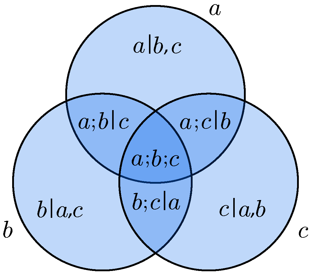
Figure 2.
Dependency diagrams for our running example systems: (A) three independent bits; (B) three completely interdependent bits; (C) independent blocks of dependent bits; and (D) the parity bit system. Regions of information zero in (A–C) are not shown.
Figure 2.
Dependency diagrams for our running example systems: (A) three independent bits; (B) three completely interdependent bits; (C) independent blocks of dependent bits; and (D) the parity bit system. Regions of information zero in (A–C) are not shown.
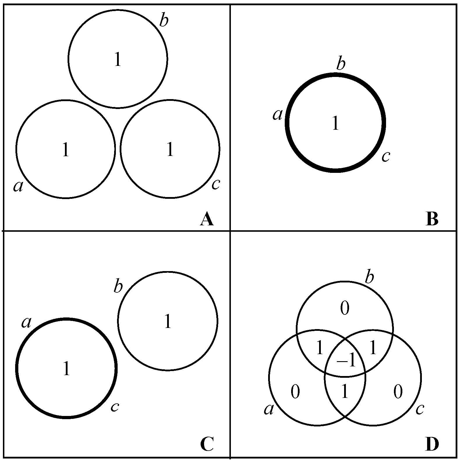
Figure 3.
Schematic illustration of the (a) complexity profile (CP) and (b) marginal utility of information (MUI) for systems with varying degrees of interdependence among components. If the components are independent, all information applies at scale 1, so the complexity profile has equal to the number of components and for . As the system becomes more interdependent, information applies at successively larger scales, resulting in a shallower decrease of . For the MUI, if components are independent, the optimal description scheme describes only a single component at a time, with marginal utility 1. As the system becomes more interdependent, information overlaps allow for more efficient descriptions that achieve greater marginal utility. For both the CP and MUI, the total area under the curve is equal to the total scale-weighted information , which is preserved under reorganizations of the system. The CP and MUI are not reflections of each other in general, but they are for an important class of systems (see Section 8).

Figure 4.
(A–D) Complexity profile for Examples A through D. Note that the total (signed) area bounded by each curve equals For Example D (the parity bit), the information at scale 3 is negative.
Figure 4.
(A–D) Complexity profile for Examples A through D. Note that the total (signed) area bounded by each curve equals For Example D (the parity bit), the information at scale 3 is negative.

Figure 5.
(A–D) Marginal Utility of Information for Examples A through D. The total area under each curve is . For Example A, all components are independent, and there is no more efficient description scheme than to describe one component at a time, with marginal utility 1. In Example B, the system state can be communicated with a single bit, with marginal utility 3. For Example C, the most efficient description scheme describes the fully correlated pair first (marginal utility 2), followed by the third component (marginal utility 1). The MUI for Example C can also be deduced from the additivity property, Equation (22). Examples A–C are all independent block systems; it follows from the results of Section 8 that their MUI functions are reflections (generalized inverses) of the corresponding complexity profiles shown in Figure 4. For Example D, the optimal description scheme is illustrated in Figure 6, leading to a marginal utility of for and for .
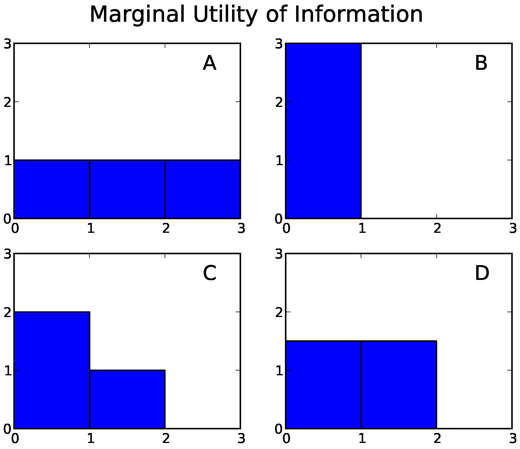
Figure 6.
Information overlaps in the parity bit system, Example D of Figure 2, augmented with a descriptor d having information content and maximal utility. Symmetry considerations imply that such a descriptor must convey an equal amount of information about each of the three components a, b and c. Constraints (i)–(iv) then yield that the amount described about each component must equal for , and 1 for . Thus the maximal utility is for , and 3 for , leading to the marginal utility given in Equation (25) and shown in Figure 5D.

Figure 7.
Stationary probability distribution for the noisy voter model [43] on a complete graph of size 10. Plot shows the probability of finding a given number i of voters in the state, for different values of the noise (mutation) parameter u, according to Equation (31). For small values of u, voters are typically in consensus ( or ); as u increases their behavior becomes more independent.

Figure 8.
(a) Complexity profile and (b) marginal utility of information (MUI) for the noisy voter model [43] on a complete graph of size 10. The MUI is approximated by computing the (exact) maximal utility of information at a discrete set of points, and then approximating . For small u, since voters are largely coordinated, much of their collective behavior can be described using small amounts of large-scale information. This leads to positive values of for large x, and large values of for small y. For large u, voters are largely independent, and therefore most information applies to one voter at a time. In this case it follows that decreases rapidly to zero, and for most values of y. For both indices, the area under each curve is 10, which is the sum of the Shannon information of each voter (i.e., the total scale-weighted information), as guaranteed by Equation (20). For all values of u, the MUI appears to take a subset of the values for .

© 2017 by the authors. Licensee MDPI, Basel, Switzerland. This article is an open access article distributed under the terms and conditions of the Creative Commons Attribution (CC BY) license (http://creativecommons.org/licenses/by/4.0/).
Share and Cite
MDPI and ACS Style
Allen, B.; Stacey, B.C.; Bar-Yam, Y. Multiscale Information Theory and the Marginal Utility of Information. Entropy 2017, 19, 273. https://doi.org/10.3390/e19060273
AMA Style
Allen B, Stacey BC, Bar-Yam Y. Multiscale Information Theory and the Marginal Utility of Information. Entropy. 2017; 19(6):273. https://doi.org/10.3390/e19060273
Chicago/Turabian StyleAllen, Benjamin, Blake C. Stacey, and Yaneer Bar-Yam. 2017. "Multiscale Information Theory and the Marginal Utility of Information" Entropy 19, no. 6: 273. https://doi.org/10.3390/e19060273
Note that from the first issue of 2016, this journal uses article numbers instead of page numbers. See further details here.