
Weak Fault Diagnosis of Wind Turbine Gearboxes Based on MED-LMD

The School of Mechanical and Power Engineering, North University of China, Xueyuan Road, Taiyuan 030051, China
*
Authors to whom correspondence should be addressed.
Entropy 2017, 19(6), 277; https://doi.org/10.3390/e19060277
Submission received: 12 April 2017
/
Revised: 2 June 2017
/
Accepted: 7 June 2017
/
Published: 15 June 2017
(This article belongs to the Special Issue Wavelets, Fractals and Information Theory III)
Abstract
:In view of the problem that the fault signal of the rolling bearing is weak and the fault feature is difficult to extract in the strong noise environment, a method based on minimum entropy deconvolution (MED) and local mean deconvolution (LMD) is proposed to extract the weak fault features of the rolling bearing. Through the analysis of the simulation signal, we find that LMD has many limitations for the feature extraction of weak signals under strong background noise. In order to eliminate the noise interference and extract the characteristics of the weak fault, MED is employed as the pre-filter to remove noise. This method is applied to the weak fault feature extraction of rolling bearings; that is, using MED to reduce the noise of the wind turbine gearbox test bench under strong background noise, and then using the LMD method to decompose the denoised signals into several product functions (PFs), and finally analyzing the PF components that have strong correlation by a cyclic autocorrelation function. The finding is that the failure of the wind power gearbox is generated from the micro-bending of the high-speed shaft and the pitting of the #10 bearing outer race at the output end of the high-speed shaft. This method is compared with LMD, which shows the effectiveness of this method. This paper provides a new method for the extraction of multiple faults and weak features in strong background noise.
1. Introduction
The wind turbine is an important piece of equipment in modern agricultural production. The health status of the gearbox directly affects the working condition of the wind turbine system. In the event of failure, it will cause huge economic losses and casualties. Therefore, technology that can diagnose its faults is highly valued [1,2,3]. Among them, the prompt fault diagnosis of the bearing is particularly important, and the bearing system’s faults mainly occur in the inner race, outer race, and rolling elements. When the bearing failure occurs, it produces periodic impulses whose characteristics depend on the location of the fault. In general, the rotational frequency or frequency multiplication of the shaft is the modulation frequency, while the fault frequency of the inner and outer race or the rolling element of the bearing is the carrier frequency. In the fault diagnosis of the actual rotating machinery and equipment, the site’s environment is relatively poor, and the measured vibration signals contain substantial noise interference besides useful characteristics. Especially for the early failure of mechanical equipment, the characteristic signals are relatively weak and often submerged by strong noise, which greatly affects the accurate acquisition of equipment status information. In order to extract the early fault features of the bearing accurately and eliminate the interference of the noise from the signal, it is necessary to suppress the noise and improve the signal-to-noise ratio.
Common denoising methods include traditional filters, wavelet denoising and Empirical Mode Decomposition (EMD), etc. With the development of wavelet theory, wavelet denoising technology can achieve a high signal-to-noise ratio in the process of signal denoising. However, the effect of wavelet denoising is largely determined by the choice of basic functions and thresholds, which often require the designer to have rich experience, and it is a non-adaptive signal processing method. Donoho and Johnstone [4,5] first proposed a scalar wavelet threshold denoising method and proved its effectiveness. However, this method ignores the correlation between the wavelet coefficients and fault features, and cannot extract the weak fault features accurately. Cai and Silverman [6] proposed a thresholding scheme that considers the nearest neighbor coefficients. The experimental results showed that the performance of the neighborhood coefficient thresholding on denoising is superior to the traditional wavelet denoising method. Ming et al. [7] proposed a method based on a cyclic Wiener filter and envelope spectrum analysis. The cyclic Wiener filter exploited the spectral coherence theory induced by the second-order cyclostationary signal. The noise component was optimally filtered by a filter-bank. The filtered signal was analyzed as an envelope spectrum. The effectiveness of the method was demonstrated on both simulated signals and actual data from a rolling bearing accelerated life test. It could be concluded that the proposed method held a great advantage in detecting early faults over single envelope analysis. Park [8] provided a method based on minimum variance cepstrum (MVC), which was introduced for the observation of periodic impulse signals under noisy environments. Using the proposed method, they found that four out of twelve newly-made bearings that passed a conventional acceptance test had small early faults in them. Moreover, comparison between these results and those obtained using other fault detection methods indicated that the MVC method was much more capable of detecting early faults under the given conditions. EMD is an adaptive signal processing method. The complex signal can be decomposed into several intrinsic mode functions (IMFs) whose instantaneous frequencies have physical significance, however, this method has the end effect, as well as modal aliasing and other shortcomings. The simulation results showed that IMFs with high frequency components after EMD are mainly composed of noise components and fault features. In the strong noise environment, the noise often affects the sensitive IMFs, and the high frequency weak characteristics can easily be submerged in the intrinsic mode function with noise. Van [9] proposed a fault feature extraction method for rolling bearing vibration signals based on non-local means (NLM) denoising, EMD and envelope detection. NLM was used as a pre-filter to filter the noise component. The denoised signal was then decomposed into a finite number of stationary IMFs by EMD. The hybrid feature extraction technique of NLM denoising, EMD, and envelope analyses successfully extracted impulsive features from noise signals.
Ensemble empirical mode decomposition (EEMD) and local mean decomposition (LMD) based denoising techniques have been widely employed recently [10,11,12,13]. LMD is an adaptive time-frequency analysis method proposed by Jonathan S. Smith. The LMD method decomposes a complex multi-component signal into a number of physical functions (PFs) from which instantaneous frequencies with physical significance can be obtained [14]. Each PF component is obtained by multiplying an envelope signal and a purely frequency modulated (FM) signal. The envelope signal is the instantaneous amplitude of the product function, and the instantaneous frequency of the product function can be obtained from the purely FM signal. The LMD method was compared with the EMD method for decomposition efficiency by Cheng [11], and the results showed the superiority of the LMD method. Then, the LMD method was applied to gear and roller bearing fault diagnosis. The analysis results demonstrated that the diagnosis approach based on LMD could identify gear and roller bearing work condition accurately and effectively. Liu [15] applied the LMD method to condition monitoring and fault diagnosis of wind turbines, and the effectiveness of the method was verified by analyzing the vibrational signals of wind turbines. However, in the strong noise environment, the actual signal is often mixed with a lot of noise which is also involved in the process of LMD decomposition, resulting in the original fault feature information and noise mixed together, so that it is not easy to extract the fault features. Moreover, the noise component increases the number of decomposition layers of LMD, which may cause the algorithm to not converge and aggravate the boundary effect. In severe cases, the LMD decomposition will lose its physical meaning, leading to misdiagnosis or leakage diagnosis. As a strong noise reduction method, MED uses the maximum kurtosis as the termination condition of the algorithm, which can highlight the strong impact component of the original signal and weaken the effect of noise on LMD.
In this approach, the MED-based denoising method is used to reduce the effect of the measurement’s noise signal. The denoised signal is then decomposed by LMD to eliminate the noise because of the effects of other components. In this paper, for the poor performance of weak signal feature extraction of rolling bearing by LMD in a strong noise environment, a method of combining of MED-based denoising and LMD has been proposed. The MED method is first employed as the pretreatment to denoise the weak signal, and the purified signal obtained through MED denoising is then decomposed by LMD into PFs. Finally, the PFs corresponding to the faulty feature signal are analyzed by cyclic autocorrelation function demodulation and the fault features are extracted.
2. Basic Theory
2.1. LMD Method
The LMD method decomposes a complex multi-component signal into a number of physical functions (PFs) from which instantaneous frequencies with physical significance can be obtained. Each PF component is obtained by multiplying an envelope signal and a purely FM signal from which a time-varying instantaneous frequency can be derived. For any given signal , the decomposition process is as follows [15]:
- (1)
- Find out all the local extrema of the original signal. The mean value of all adjacent local extrema points and can be determined byAll successive mean points are plotted by a straight line and then smoothed by the moving average method to obtain the local mean function .
- (2)
- The local is obtained byThe local envelope estimation values are smoothed in the same way and to the same degree as the local means to form a continuous envelope function .
- (3)
- The local mean function is separated from the original signal .
- (4)
- The is then divided by to be demodulatedRepeat the above steps, the envelope estimation function of can be calculated. If , then is not regarded as a purely frequency modulated signal. This iteration process continues times until a purely frequency modulated signal is obtained. The iteration steps are as followswhereThe iteration termination condition isIn practical applications, in order to reduce the number of iterations and the operation time without affecting the decomposition effect, the iteration termination condition can be simplified as
- (5)
- The envelope signal (instantaneous amplitude function) is obtained by multiplying all the envelope estimation functions generated in the iterative process.
- (6)
- The envelope signal and the pure FM signal are multiplied to obtain the first PF component of the original signal.The PF contains the highest frequency components of the original signal. Meanwhile, it is a mono-component AM-FM signal, whose instantaneous amplitude is exactly the envelope signal and the instantaneous frequency can be obtained from the pure frequency modulated signal .
- (7)
- The first PF component is separated from the original signal to obtain a new signal , which will act as the new original data to repeat the above steps. The number of iterations is until u1(t) becomes a monotonic function.The original signal can be reconstructed by all the PF components and uk, that is
The result shows that the LMD decomposition does not cause the loss of the information of the original signal.
2.2. MED Method
The minimum entropy deconvolution (MED) was first proposed by Ralph Wiggins, and is an adaptive system identification method. Sawalhi [16] first used MED for rolling bearing and gear fault diagnosis in 2007. The basic principle of MED is to solve the deconvolution results to highlight a few large spikes, which is a necessary prerequisite for MED. The maximum kurtosis is used as the iteration termination condition. According to the maximum principle of kurtosis, the greater the kurtosis value, the greater the proportion of the impact component in the signal. This feature is very suitable for the noise reduction of rotating machinery impact failure because it can better highlight the shock pulse. Assuming that the rolling bearing failure signal can be expressed as:
In order to facilitate the analysis, is removed from the Equation (14). If is the impact sequence of the rolling bearing, the source signal characteristics will be lost after decays to , due to the environmental noise and path transmission, resulting in a large entropy change. The purpose of solving for deconvolution is to obtain an inverse filter that recovers the property of the input according to the output, which is
is an estimate of , and its optimality is determined by the sequence obtained by solving deconvolution of Equation (15). The closer the shape of the sequence to the shape of , f(x) is optimal. This method is called minimum entropy deconvolution because the inverse filter can make restore the original property or have most of the original properties, that is, to minimize the entropy. Wiggins used the norm of sequence to determine the entropy of itself and used it as the objective function to solve the optimal solution. Therefore, the purpose of minimum entropy deconvolution is to find the optimal inverse filter.
The optimal inverse filter maximizes the norm , which is
It can be seen from Equation (15) that
where: L is the length of the inverse filter whose unit is 1, and take the derivative of the Equation (7) on both sides
From the Equation (19) and the Equation (17), it can be obtained as
The Equation (20) written in matrix form is
A is the autocorrelation matrix of sequence , and can be expressed as
According to the above analysis, we can sum up the minimum entropy recursive iterative algorithm, and the iterative steps are as follows:
- (1)
- The elements in are all initialized to 1.
- (2)
- The iterative calculation of the equation is performed.
- (3)
- Calculate .
- (4)
- Calculate .
- (5)
- If is less than a given threshold (the threshold of this paper is 0.01), recursion is stopped. Otherwise, let increase by 1, and return to step 2.
3. A Bearing Fault Diagnosis Method Based on MED-LMD
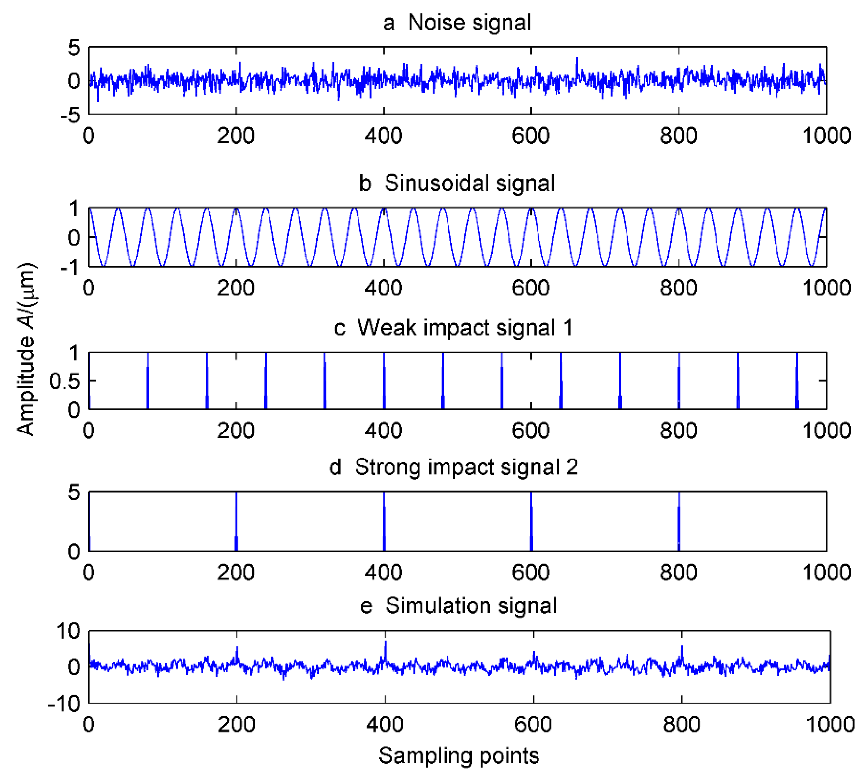
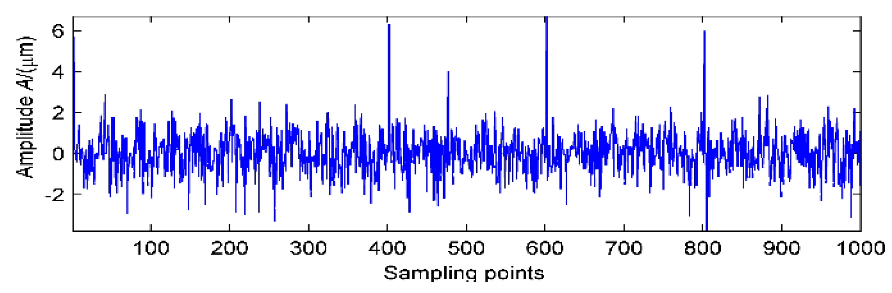
In view of the problem that the early fault vibration signal of the rolling bearing is weak and the fault feature is difficult to extract in the strong white noise environment, a hybrid method is proposed in this paper. The MED method is first employed as the pretreatment to denoise the weak signal, and the purified signal obtained through the MED denoising is then decomposed by LMD to eliminate the noise arising from the effects of other components. The merit of the MED method is that it has a strong denoising ability in a strong noise environment, and it has obvious self-adaptability. The purpose of the MED method is to deconvolute the results to highlight a few large spikes, with the maximum kurtosis value as the termination condition of the calculation. The weak early fault feature extraction is not ideal because early fault features can easily be submerged in the denoised signal. In order to reflect the noise reduction capability of this method, we took the simulation signal containing strong noise as an example, and analyzed it. The time-domain signal is shown in Figure 1 which contains a noise signal, a sinusoidal signal, a weak impact (signal 1), and a strong impact (signal 2). After filtering the simulation signal using MED, the kurtosis value increased from 1.47 to 5.562. The results are shown in Figure 2. Most of the strong shock signals are highlighted, while the weak shock signal was still submerged in the noise.
LMD is a very effective fault signal processing method because of its high efficiency of decomposition and good processing of non-stationary signals. However, due to the strong noise interference, the number of decomposed layers of LMD will increase in the decomposition process of the actual vibration signal, and even lead to a greater deviation between the decomposition result and the ideal result, thus affecting the fault diagnosis analysis as shown in the third part of the simulation signal. Therefore, there is an urgent need to find a suitable signal denoising method to improve the decomposition accuracy of LMD, reduce the number of decomposition layers, and increase the signal-to-noise ratio of the input signal.
In order to improve the signal-to-noise ratio and highlight the weak fault impact component, the signal is pretreated with the MED method to weaken the effect of noise on the weak impact component, that is, the effect of the decomposition efficiency of LMD. The LMD algorithm is then used for secondary noise reduction. Considering that each PF component is obtained by multiplying an envelope signal with a pure FM signal, the cyclic autocorrelation function is used to process the denoised sensitive PF components. This method overcomes the limitations of LMD in strong background noise. An example analysis is shown in Section 3 and Section 4, and the specific flow chart is illustrated in Figure 3.
4. Modulation Signal Analysis Based on MED-EEMD and Cyclic Autocorrelation Function
When a bearing fails, the vibration signal is often expressed as the modulation signal [6]. The fault signal demodulation analysis is designed to extract the vibration signal fault characteristics. For example, given a modulation signal (23), the carrier signal is weaker than the noise signal, the signal is digitized at a sampling frequency of 2000 Hz and the number of data samples is 1000. The two modulation frequencies , are 50 Hz and 30 Hz, respectively, and the carrier frequency is 180 Hz.
The simulation signal is represented in Figure 4a. It can be seen from the graph that the carrier and the modulation signal are completely submerged by noise. In order to extract the frequency components of these signals, the simulation signal is denoised by the MED method. The kurtosis values before and after noise reduction were 0.1192 and 1.9154, respectively. The kurtosis value increased 16-fold, and the noise reduction effect is obvious. There are only individual peaks in the signal, and no clear periodic components appear, which is the limitation of MED. Simultaneously, the cyclic autocorrelation demodulation of the simulation signal and the MED-based denoised signal were performed, as shown in Figure 4b. The spectrum peak does not appear at the high and low frequencies of the carrier frequency and the modulation frequency, but after MED noise reduction and then cyclic autocorrelation function demodulation analysis, the spectrum peak has increased in the case of = 50 Hz and Hz. However, the carrier frequency at high frequencies still cannot be distinguished. In the case of strong noise, MED noise reduction and cyclic autocorrelation function demodulation cannot extract the characteristic frequency accurately.
In order to show the interference of the noise to the weak signal in the original signal by EEMD decomposition, the original signal is decomposed by LMD, as shown in Figure 5a. The first three layers of PFs which have the strongest correlation with the original signal were obtained, and cyclic autocorrelation demodulation analysis was carried out on them, as shown in Figure 6a–c. The modulation frequency = 50 Hz and the carrier frequency = 360 Hz only appear in the second layer. And the spectrum peak is not so prominent that it can be easily confused with other components. At the same time, the modulation frequency = 30 Hz also does not appear. It is clear that the original signal denoising processing is necessary. The results of LMD decomposition of the signal after MED noise reduction are shown in Figure 5b. The first three layers are analyzed by cyclic autocorrelation function, and the results are shown in Figure 6d–f. In the high frequency zone, the carrier frequency = 360 Hz is obviously prominent, 310 Hz, 330 Hz, 410 Hz are side frequencies of the frequency 360 Hz, respectively. Their spacing is the modulation frequency = 50 Hz and = 30 Hz. In the low frequency zone, = 50 Hz and = 30 Hz are the modulation frequencies of the original signal. Therefore, noise reduction by MED can not only avoid the effect of noise on the weak features, but also does not affect the decomposition effect of LMD. Although the MED method cannot extract the weak feature frequency signal directly, using its noise reduction ability to eliminate the influence of the original signal noise on LMD decomposition effect helps the LMD method to identify the weak feature components. This method is not only unique in that the original signals are analyzed by cyclic autocorrelation function demodulation, but is also superior to the method in which MED-based and LMD-based de-noising signals are analyzed by cyclic autocorrelation function demodulation.
5. Vibration Signal Analysis
The method is further demonstrated with a vibration signal from a wind turbine. The test bench sketch of a wind turbine gearbox is shown in Figure 7. The speed-increasing gear transmission system has a three-stage gear transmission device with the generator as the load of the gearbox. During the test, as the power of the generator increases, the vibration and noise of the gearbox are continuously strengthened, and the temperature of the high-speed shaft continues to rise. In order to determine the fault location, we use acceleration sensors and a dynamic signal analyzer for measurement and data acquisition. The sampling points are located in the bearing block of the high-speed shaft gearbox. The signal is digitized at a sampling frequency of 10,000 Hz and the number of data sample is 2048. The rotating speed of the output gear shaft is 1728 r/min and the rotating frequency of the shaft is 28.8 Hz (modulation frequency). The position of the high-speed shaft, the speed of the bearing and the frequency of the fault are shown in Table 1
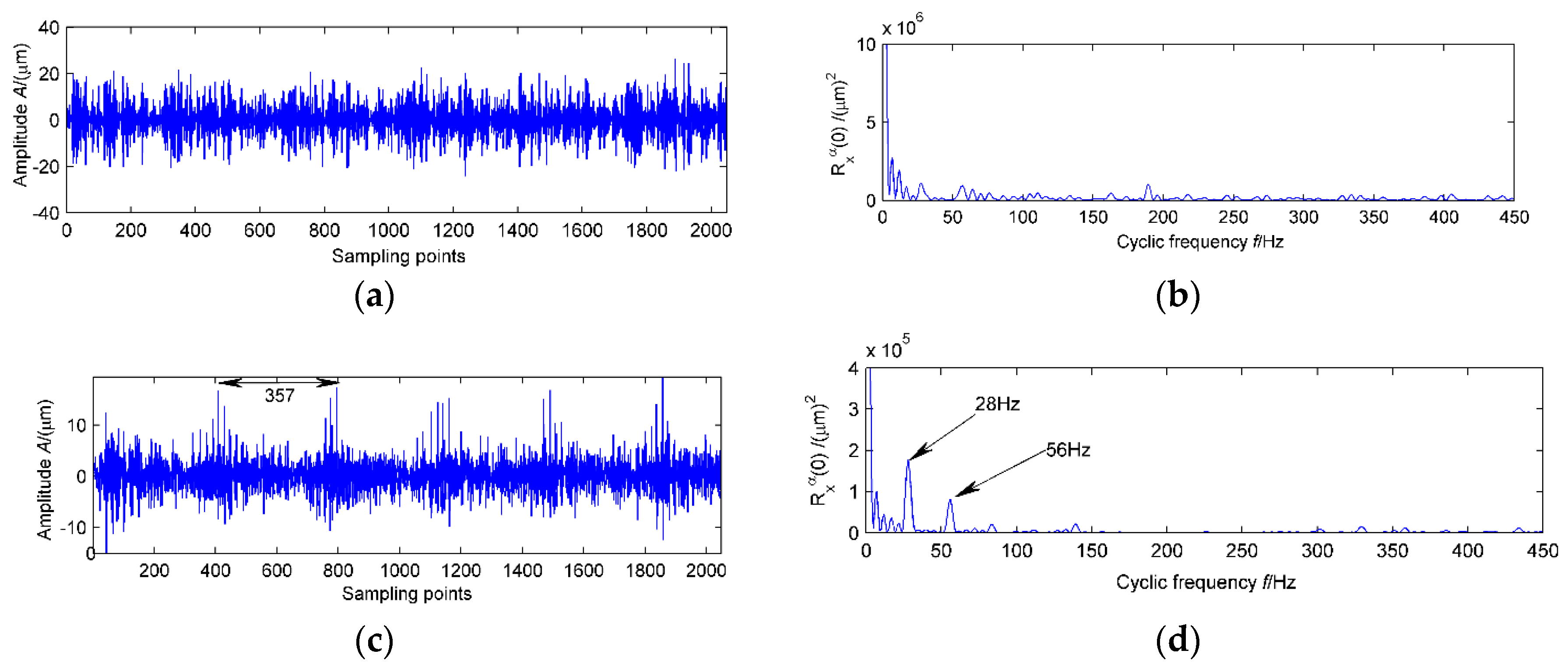
The original vibration signal shown in Figure 8a is chaotic and has no obvious periodic component. After cyclic autocorrelation demodulation analysis, no significant carrier and modulation frequencies appear in Figure 8b. The results of noise reduction of the original signal by MED are shown in Figure 8c. It can be seen from the figure that the signal-to-noise ratio is obviously increased after denoising and the periodic impulse is prominent. There are about 357 sampling points between the two adjacent impulse signals. The corresponding frequency 1/0.0357 = 28.01 Hz is the rotation frequency of the high-speed shaft. The cyclic autocorrelation function of the vibration signal, illustrated in Figure 8d, consists of two main frequency components at 28 Hz and 56 Hz, which correspond respectively to the high-speed shaft rotational frequency and its second-order harmonics. It can be initially determined that there appears to be a weak bending on the high-speed shaft.
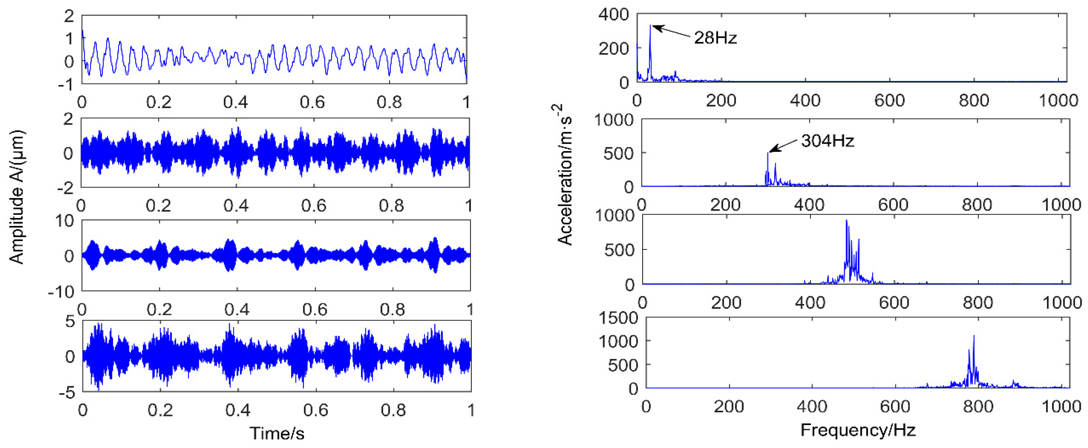
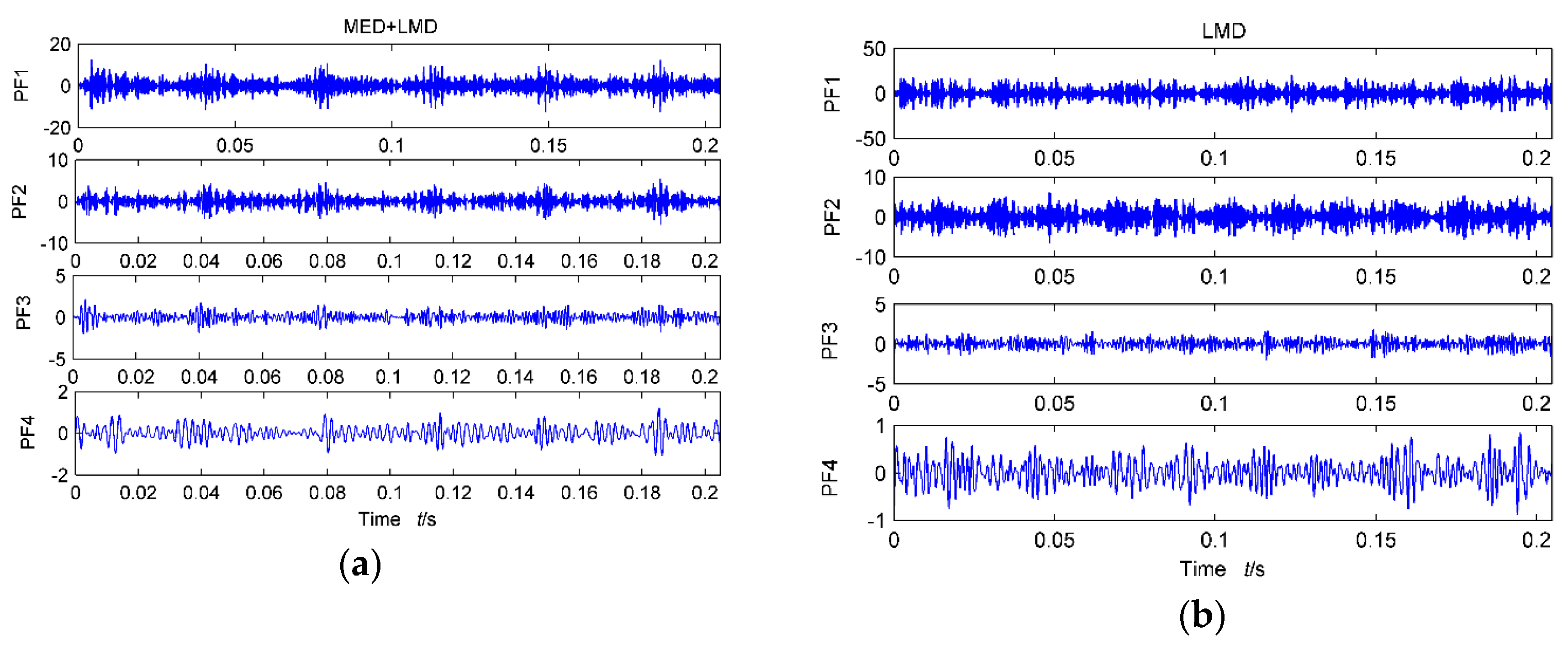
In order to further determine the characteristic frequency of the fault, the signal after MED noise reduction is decomposed by LMD, and the decomposition result is shown in Figure 9a. The main energy of the original signal is concentrated in the first four layers, among which the first layer is of the strongest correlation with the original signal. The first four PFs are analyzed by cyclic autocorrelation function demodulation, and the result is represented in Figure 10a–d. The first four PFs contain the strong impact component of the original signal, that is, the high-speed shaft rotational frequency and its second order harmonics. Modulation frequency (high-speed shaft rotating frequency) is still the main frequency in the low frequency zone in the second two layers. A frequency cluster with a center frequency of 304 Hz and a rotational frequency of the high-speed shaft as a side band appears in the high frequency zone. The frequency of 304 Hz is also second-order harmonics of the fault frequency of the bearing outer ring at the output end of the #10 bearing. The presence of these prominent frequency components indicates that there is slight pitting on the face of outer rings of the #10 bearings at the end of the of high-speed shaft.
When opening the box, it can be found that the high-speed shaft has a small bending deformation and there is pitting on the face of outer rings of the #10 bearings at one side end of the high-speed shaft. Thus, the diagnosis result has been confirmed. As the vibration signal generated by the bearing outer ring pitting is weak, it is easily submerged by the noise. The first four layers of PFs of the measured signal are analyzed by LMD, and the results are shown in Figure 9b. The cyclic autocorrelation functions of first four PFs are shown in Figure 10e–h. As can be seen from the figures, the low frequency is still dominated by the modulation frequencies, but the fault frequency of the bearing outer ring at the output end of the #10 bearing is not reflected in the high frequency zone. Therefore, it is not ideal to use only the LMD decomposition method to extract the weak fault signal in a strong noise background. However, a hybrid fault diagnosis method based on the MED denoising, LMD, and the cyclic autocorrelation function can successfully extract the weak characteristic frequency. The analyzed results demonstrate that the proposed method is an effective approach in identifying multiple faults in rotating machinery.
In order to compare and analyze the proposed method, an adaptive noise reduction method, variational mode decomposition (VMD), is used to further analyze the vibration signals, and the results were compared with EMD, EEMD, and other adaptive methods. VMD has the advantages of fast convergence, good noise robustness, and so on. In addition, this method has different frequency bands for each layer of intrinsic modal functions, so it is suitable for multi-fault feature extraction. Similarly, a MED + VMD secondary noise reduction method was used to process the original signal and the result is shown in Figure 11. Through the analysis of the first four layers of IMFs, each layer corresponds to a periodic component, of which the first two layers correspond to the fault characteristics. The corresponding frequencies of the other two layers are pseudo frequencies, however, belonging to the noise components. Although this method can also identify the fault characteristics, the efficiency of VMD noise reduction is affected by two factors; one is the penalty factor and the other is the number of decomposition layers. Too few layers will cause modal aliasing, too many layers will result in energy leakage. The penalty factor was set to 5000, and the number of decomposition layers was set to 4. The results are shown in Figure 11. The rationality of the proposed method is verified by the comparison of the two methods.
6. Conclusions
(1) The PFs obtained by LMD decomposition not only contain the characteristic frequency, but also the noise components. In the strong noise background, the weak feature information is still submerged in the noise and is difficult to extract.
(2) MED has a strong capability for noise reduction and filtering, but can only highlight a few large spikes. Thus, the original signal through the MED filter, can only increase the kurtosis value of the signal and the weak characteristic frequency still cannot be extracted.
(3) A hybrid fault diagnosis method based on MED denoising and the LMD method is proposed in this paper. The filtering with MED reduces the influence of noise on LMD, and through cyclic autocorrelation demodulation analysis, the weak feature is successfully extracted. The proposed method was applied to analyze measured vibration signals and simulated signals. The results demonstrate the feasibility of the proposed method. In general, the MED-LMD method provides a new idea for weak fault diagnosis of rotating machinery, which is helpful for further research and has certain reference value.
Acknowledgments
This work was supported by the Natural Science Foundation of Shanxi Province, China and Science and technology Foundation of Shanxi Provincial (No. 2015011063).
Author Contributions
Zhijian Wang and Junyuan Wang conceived and designed the experiments; Zhijian Wang, Shaohui Ning
and Yanfei Kou performed the experiments; Zhijian Wang and Jiping Zhang analyzed the data and contributed reagents/materials/analysis tools; Zhijian Wang and Zhifang Zhao wrote the paper.
Conflicts of Interest
The authors declare no conflict of interest.
References
- Wu, S.D.; Wu, C.W.; Wu, T.Y.; Wang, C.C. Multi-scale analysis based ball bearing defect diagnostics using mahalanobis distance and support vector machine. Entropy 2013, 15, 416–433. [Google Scholar] [CrossRef]
- Zhang, L.N.; Wang, Y.; Wu, K.; Sheng, R.Y.; Huang, Q.L. Dynamic modeling and vibration characteristics of a two-stage closed-form planetary gear train. Mech. Mach. Theory 2016, 97, 12–28. [Google Scholar] [CrossRef]
- Shi, Z.L.; Song, W.Q.; Taheri, S. Improved LMD, permutation entropy and optimized K-means to fault diagnosis for roller bearings. Entropy 2016, 18, 1–11. [Google Scholar] [CrossRef]
- Donoho, D. Denoising via Soft Thresholding. IEEE Trans. Inf. Theory 1995, 43, 613–627. [Google Scholar] [CrossRef]
- Donoho, D. Ideal spatial adaptation via wavelet shrinkage. Biometrika 1994, 83, 425–455. [Google Scholar] [CrossRef]
- Cai, T.T.; Silverman, B.W. Incorporating information on neighboring coefficients into wavelet estimation. Sankhya 1999, 63, 127–148. [Google Scholar]
- Ming, Y.; Chen, J.; Dong, G. Weak fault feature extraction of rolling bearing based on cyclic Wiener filter and envelope spectrum. Mech. Syst. Signal Process. 2011, 25, 1773–1785. [Google Scholar] [CrossRef]
- Park, C.S.; Choi, Y.C. Early fault detection in automotive ball bearings using the minimum variance cepstrum. Mech. Syst. Signal Process. 2013, 38, 534–548. [Google Scholar] [CrossRef]
- Van, M.; Kang, H.J.; Shin, K.S. Rolling element bearing fault diagnosis based on non-local means denoising and empirical mode decomposition. IET Sci. Meas. Technol. 2014, 8, 571–578. [Google Scholar] [CrossRef]
- Chen, X.Y.; Shen, C. Study on temperature error processing technique for fiber optic gyroscope. Optik 2013, 124, 784–792. [Google Scholar] [CrossRef]
- Han, J.J.; Mirko, V.D.B. Microseismic and seismic denoising via ensemble empirical mode decomposition and adaptive thresholding. Geophysics 2015, 80, KS68–KS80. [Google Scholar] [CrossRef]
- Sun, J.D.; Xiao, Q.Y.; Wen, J.T.; Zhang, Y. Natural gas pipeline leak aperture identification and location based on local mean decomposition analysis. Measurement 2016, 79, 147–157. [Google Scholar]
- Cheng, J.; Yang, Y.; Yang, Y. A rotating machinery fault diagnosis method based on local mean decomposition. Digit. Signal Process. 2012, 22, 356–366. [Google Scholar] [CrossRef]
- Smith, J.S. The local mean decomposition and its application to EEG perception data. J. R. Soc. Interface 2005, 2, 443–454. [Google Scholar] [CrossRef] [PubMed]
- Liu, W.Y.; Zhang, W.H.; Han, J.G.; Wang, G.F. A new wind turbine fault diagnosis method based on the local mean decomposition. Renew. Energy 2012, 48, 411–415. [Google Scholar] [CrossRef]
- Sawalhi, N.; Randall, R.B.; Endo, H. The enhancement of fault detection and diagnosis in rolling element bearings using minimum entropy deconvolution combined with spectral kurtosis. Mech. Syst. Signal Process. 2007, 21, 2616–2633. [Google Scholar] [CrossRef]
Figure 1.
Simulation signal.

Figure 2.
Using minimum entropy deconvolution (MED) noise reduction.

Figure 3.
Flow chart of the proposed weak fault diagnosis method.
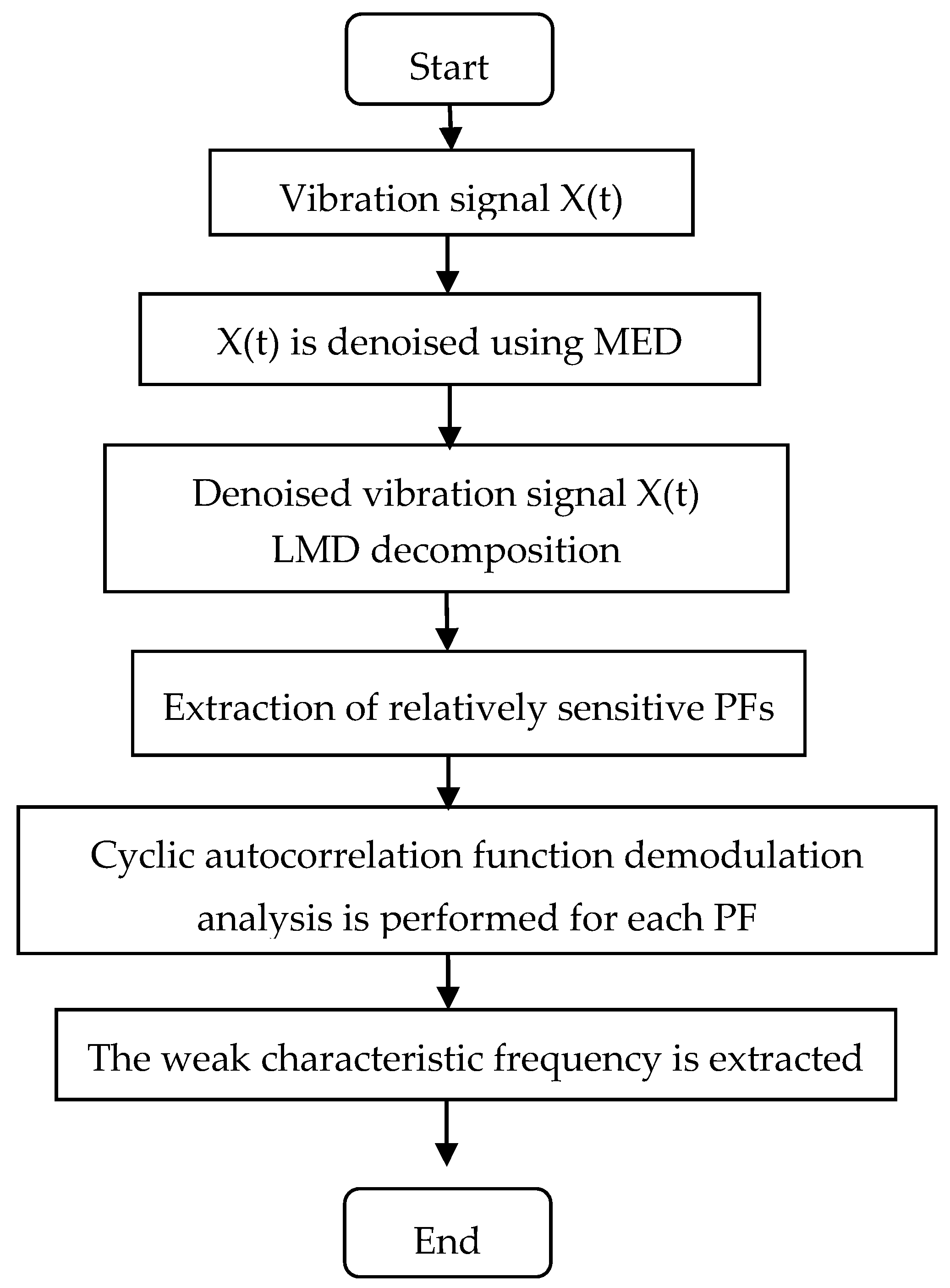
Figure 4.
Waveform figure and cyclic autocorrelation function when = 0 of simulation signal and noise reduction by MED. (a) Simulation signal and noise reduction by MED; (b) Cyclic autocorrelation function when = 0 of simulation signal and noise reduction by MED.
Figure 4.
Waveform figure and cyclic autocorrelation function when = 0 of simulation signal and noise reduction by MED. (a) Simulation signal and noise reduction by MED; (b) Cyclic autocorrelation function when = 0 of simulation signal and noise reduction by MED.
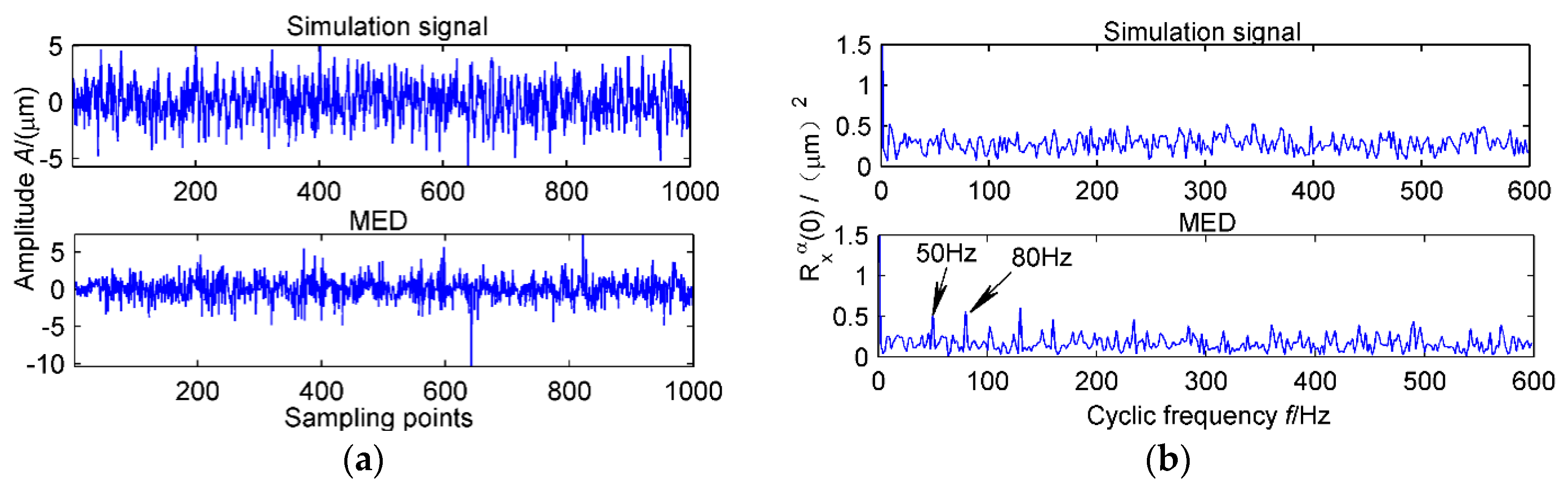
Figure 5.
First, three intrinsic mode functions (IMFs) results using ensemble empirical mode decomposition (EEMD) and MED + EEMD. (a) First three IMFs results using EEMD; (b) First three IMFs results using MED + EEMD.
Figure 5.
First, three intrinsic mode functions (IMFs) results using ensemble empirical mode decomposition (EEMD) and MED + EEMD. (a) First three IMFs results using EEMD; (b) First three IMFs results using MED + EEMD.

Figure 6.
Cyclic autocorrelation function when = 0 for first three IMFs from local mean decomposition (LMD) and MED + LMD. (a) Cyclic autocorrelation function when = 0 for PF1 from LMD; (b) Cyclic autocorrelation function when = 0 for PF2 from LMD; (c) Cyclic autocorrelation function when = 0 for PF3 from LMD; (d) Cyclic autocorrelation function when = 0 for PF1 from MED + LMD; (e) Cyclic autocorrelation function when = 0 for PF2 from MED + LMD; (f) Cyclic autocorrelation function when = 0 for PF3 from MED + LMD.
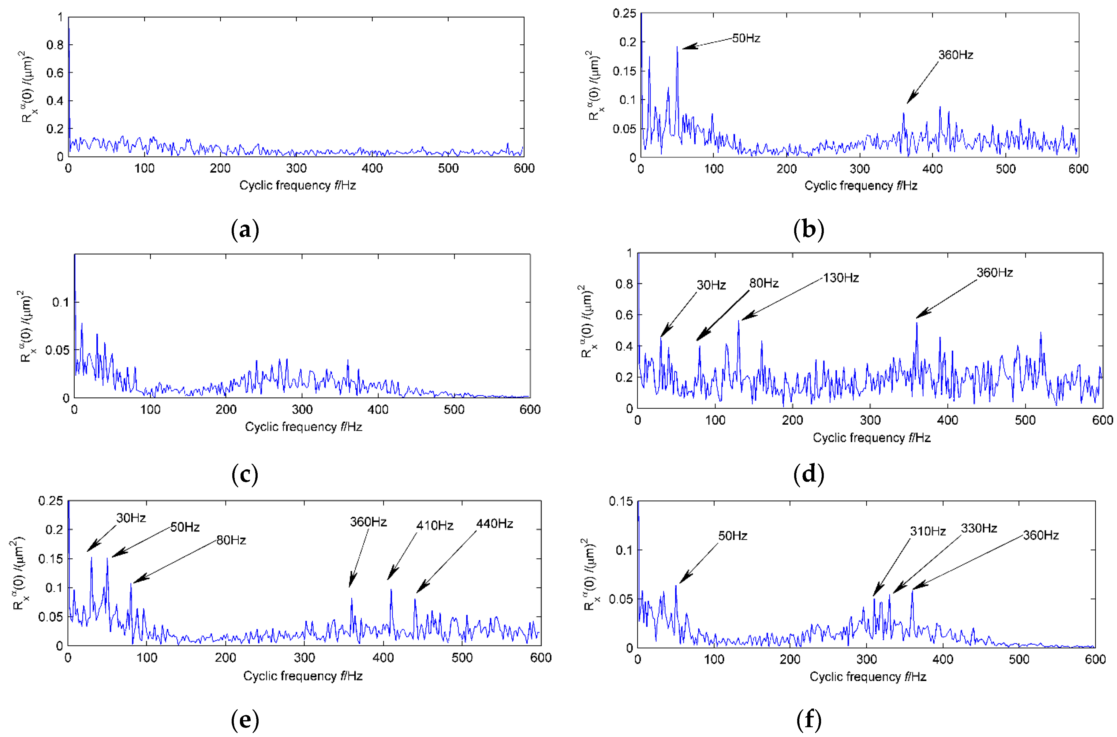
Figure 7.
Schematic of a wind turbine gearbox test rig.
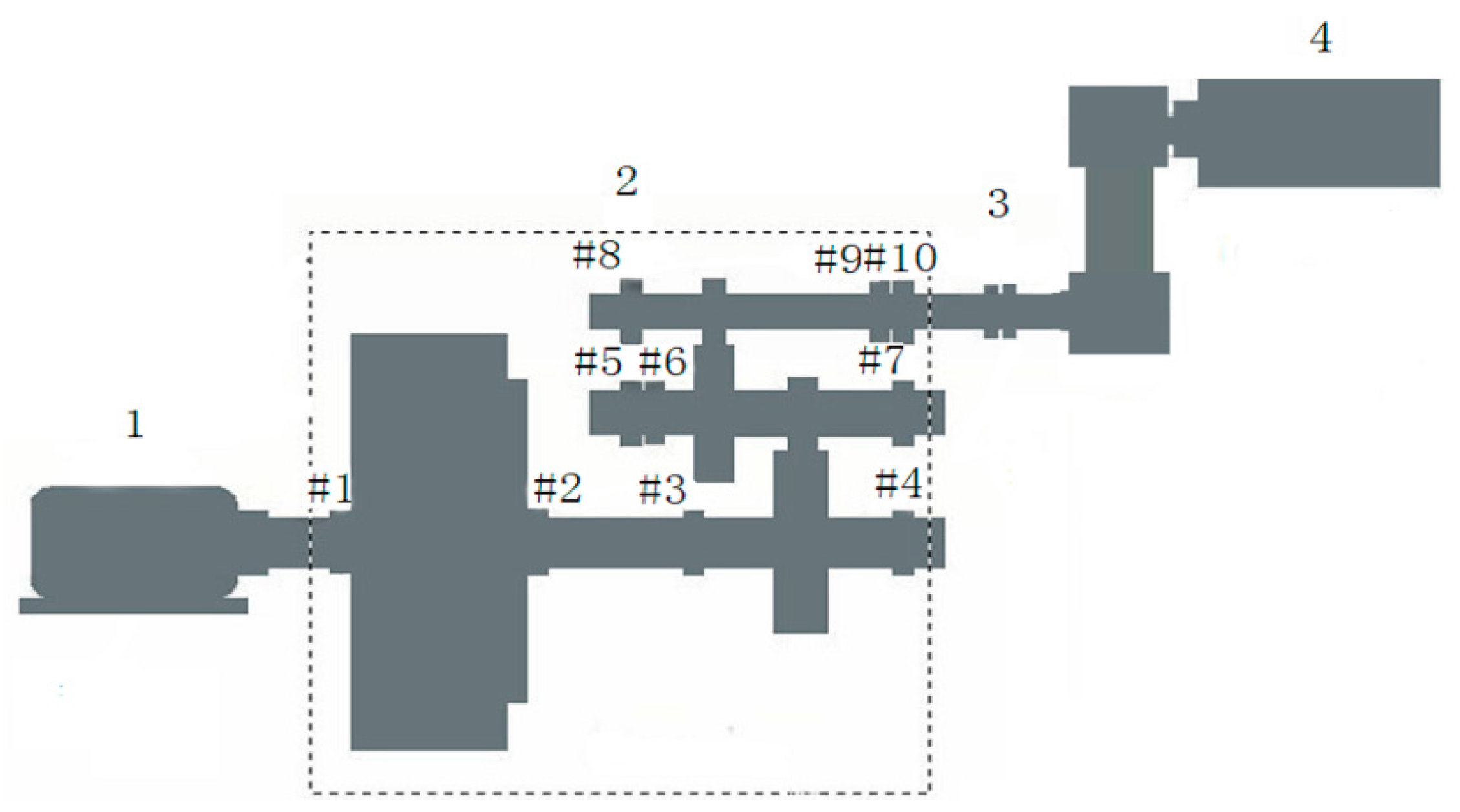
Figure 8.
Original vibration signal and signal after noise reduction by MED and their cyclic autocorrelation function when = 0. (a) Vibration signal; (b) Cyclic autocorrelation function for Vibration signal when = 0; (c) Vibration signal noise reduction by MED; (d) Cyclic autocorrelation function when = 0 after noise reduction by MED.

Figure 9.
Results of the first four PFs using LMD and MED + LMD. (a) Results from the first four IMFs of the vibration signal using MED + LMD; (b) results of the first four IMFs of the vibration signal using LMD.
Figure 9.
Results of the first four PFs using LMD and MED + LMD. (a) Results from the first four IMFs of the vibration signal using MED + LMD; (b) results of the first four IMFs of the vibration signal using LMD.

Figure 10.
Cyclic autocorrelation function of the vibration signal when = 0 for the first four IMFs from EEMD and MED + EEMD. (a) Cyclic autocorrelation function when = 0 for PF1 from MED + LMD; (b) Cyclic autocorrelation function when = 0 for PF2 from MED + LMD; (c) Cyclic autocorrelation function when = 0 for PF3 from MED + LMD; (d) Cyclic autocorrelation function when = 0 for PF4 from MED + LMD; (e) Cyclic autocorrelation function when = 0 for PF1 from LMD; (f) Cyclic autocorrelation function when = 0 for PF2 from LMD; (g) Cyclic autocorrelation function when = 0 for PF3 from LMD; (h) Cyclic autocorrelation function when = 0 for PF4 from LMD.
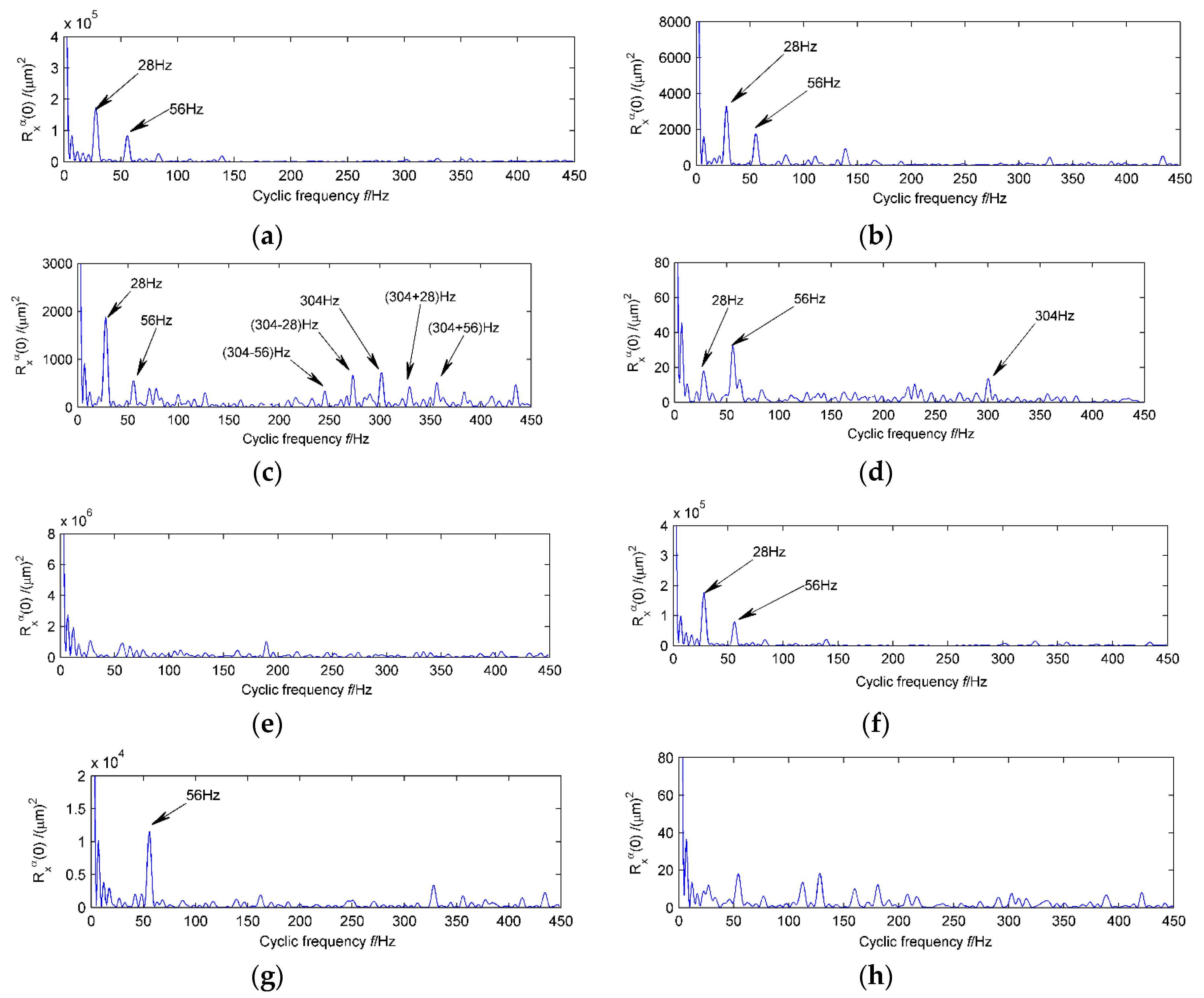
Figure 11.
Vibration signal four IMFs from MED + VMD and envelope spectrum.

Table 1.
Bearing fault period data.
| Bearing Locations | Inner Ring Fault Period | Outer Ring Fault Period | Rolling Element Fault Period |
|---|---|---|---|
| High speed input shaft bearing #8 | 42.3 | 59.9 | 100.4 |
| High speed input shaft bearing #9 | 42.3 | 59.9 | 100.4 |
| High speed output shaft bearing #10 | 45.1 | 65.5 | 108.3 |
© 2017 by the authors. Licensee MDPI, Basel, Switzerland. This article is an open access article distributed under the terms and conditions of the Creative Commons Attribution (CC BY) license (http://creativecommons.org/licenses/by/4.0/).
Share and Cite
MDPI and ACS Style
Wang, Z.; Wang, J.; Kou, Y.; Zhang, J.; Ning, S.; Zhao, Z. Weak Fault Diagnosis of Wind Turbine Gearboxes Based on MED-LMD. Entropy 2017, 19, 277. https://doi.org/10.3390/e19060277
AMA Style
Wang Z, Wang J, Kou Y, Zhang J, Ning S, Zhao Z. Weak Fault Diagnosis of Wind Turbine Gearboxes Based on MED-LMD. Entropy. 2017; 19(6):277. https://doi.org/10.3390/e19060277
Chicago/Turabian StyleWang, Zhijian, Junyuan Wang, Yanfei Kou, Jiping Zhang, Shaohui Ning, and Zhifang Zhao. 2017. "Weak Fault Diagnosis of Wind Turbine Gearboxes Based on MED-LMD" Entropy 19, no. 6: 277. https://doi.org/10.3390/e19060277
Note that from the first issue of 2016, this journal uses article numbers instead of page numbers. See further details here.