The Mehler-Fock Transform in Signal Processing


1
Department of Electrical Engineering, Linköping University, SE-581 83 Linköping, Sweden
2
Department of Science and Technology, Linköping University, SE-60174 Norrköping, Sweden
Entropy 2017, 19(6), 289; https://doi.org/10.3390/e19060289
Submission received: 25 April 2017
/
Revised: 13 June 2017
/
Accepted: 15 June 2017
/
Published: 20 June 2017
(This article belongs to the Special Issue Information Geometry II)
Abstract
:Many signals can be described as functions on the unit disk (ball). In the framework of group representations it is well-known how to construct Hilbert-spaces containing these functions that have the groups SU(1,N) as their symmetry groups. One illustration of this construction is three-dimensional color spaces in which chroma properties are described by points on the unit disk. A combination of principal component analysis and the Perron-Frobenius theorem can be used to show that perspective projections map positive signals (i.e., functions with positive values) to a product of the positive half-axis and the unit ball. The representation theory (harmonic analysis) of the group SU(1,1) leads to an integral transform, the Mehler-Fock-transform (MFT), that decomposes functions, depending on the radial coordinate only, into combinations of associated Legendre functions. This transformation is applied to kernel density estimators of probability distributions on the unit disk. It is shown that the transform separates the influence of the data and the measured data. The application of the transform is illustrated by studying the statistical distribution of RGB vectors obtained from a common set of object points under different illuminants.
1. Introduction
Fitting statistical models to empirical data is one of the most fundamental techniques in signal processing. Usually, one distinguishes between parametric and non-parametric models. Parametric models require, by definition, information about the type of the underlying statistical distribution. Non-parametric methods are more data-driven. Two important classes of non-parametric techniques are histograms and kernel-density estimators. Histograms are computationally very efficient but the specification of the bins used can be very difficult. Kernel density estimators, on the other hand, require only the definition of the kernel. One of the drawbacks of a straight-forward implementation of a kernel density estimator is the fact that a new data point to be included into the analysis can interact with a large number of already analysed data points.
In cases where the underlying domain has a group theoretical structure methods from harmonic analysis can be used to separate the contributions from the kernel and the data. In the following this will be illustrated in the case where the domain on which the data is defined is the unit disk and where the symmetry group of the data is the group SU(1,1) (to be introduced later). In the harmonic analsis framework the simplest groups are the commutative groups which lead to ordinary Fourier transforms. Next come the non-commutative but compact groups like the rotation groups which are related to finite-dimensional invariant subspaces and corresponding series expansions (like the spherical harmonics). The group SU(1,1) is the simplest example of a non-commutative and non-compact group and the corresponding Fourier transform is an integral transform, the Mehler-Fock transform to be described in the following sections.
The group SU(1,1) is well-known in mathematics and theoretical physics but there are only a few applications in signal processing. One reason for this is certainly that the usage of the unit disk domain is not as obvious as those of other domains. The natural domain for time-sequences is the real line with the shift-operators as symmetry group. The plane or three-dimensional space are domains for spatial processes with spatial shifts of the origin of the space as group elements. The rotation group is related to unit spheres and orientations. In the next section it will be shown that stochastic processes with positive values only have a natural conical structure with SU(1,1) as the natural symmetry group. Then the main results regarding the Mehler-Fock transform will be presented and a few properties of the transform will be illustrated with the help of an application from color signal processing.
2. Positive Signals
The raw output values of many measurement processes are non-negative numbers. An extreme example are binary measurements indicating the absence/presence of a response. This is typical for biological and binary technical systems. Other common examples are size, weight, age/duration or the photon counts of a camera. For simplicity only the case of strictly positive measurements will be considered. This is is natural in many cases. In imaging science, for example, measurements are often representing counts such as the number of interactions of photons with the sensor in a given time interval. Sensors are never perfect and the cases where zero counts are registered should be very rare. The measurement values are therefore almost always positive numbers.
In the following functions (signals) that are outcomes of stochastic processes are considered. It is assumed that they are elements of a vector (or Hilbert) space and that they assume positive values only. In this space one can use principal component analysis to introduce a basis where the first eigenvector has only positive components. This follows from the Perron-Frobenius (Krein-Milman) theorem. In the following only processes will be considered in which the first eigenvector is (approximately) proportional to the mean vector. It is also assumed that all relevant signals lie in a conical subset which is a product of the positive half-axis and the n-dimensional solid unit ball. In the following only the case where denotes the unit disk is considered. Generalizations to higher dimensions are straight-forward.
This is formulated in the following definition:
Definition 1.
A positive stochastic process is a function where ω is the stochastic variable and denotes a set on which the function is defined. For every ω the function is an element in a Hilbert space with scalar product .
Typical examples of are:
- a set of points on the plane which describe the location of the th sensor element (pixel)
- a set of points in a time-interval denoting the time when the measurement was obtained
- a set of indices describing the spectral sensitivity of color sensor number k.
For a positive stochastic process f the expectation and the correlation function are defined as usual:
Definition 2.
The expectation is defined as .
The correlation function is defined as .
The correlation function defines an integral operator defined as:
The correlation function is symmetric, i.e., and for all positive stochastic processes the expectation and the correlation function have positive values everywhere. For a finite set the expectation is a vector and the correlation function is a symmetric positive matrix (having only positive elements) which is also positive semi-definite.
The operator is a positive and positive-definite operator and the Krein-Rutman theorem (Perron-Frobenius theorem in the case of matrices) shows that the first eigenfunction of the operator is a positive function. All eigenvalues are non-negative. Denote the eigenfunctions of (sorted by decreasing eigenvalues) as . Then
The following example, discussing a model of an RGB camera, should give an idea of a situation in which the unit disk model arises in signal processing. A more general and detailed application is discussed later when the properties of the Mehler-Fock transform are illustrated. In a first approximation it is assumed that such a camera acts as a linear system and that the measured RGB values are linearly related to the incoming light. In practice this implies using the raw data from the camera sensor, excluding processing steps like white-balancing and gamma mapping. Also excluded are, in this first step, pixels outside the linear response region of the camera avoiding critical effects such as a saturation of the sensor. This will be discussed later in connection with the experiments. Under these conditions the doubling of the exposure time will thus result in a multiplication of the RGB vector by a factor of two.
Under this condition the group of positive real numbers acts on an RGB vector as . The elements of the group are intensity transformations and is defined as the intensity of the RGB vector The result z of the projection defines the chroma of the RGB vector .
The main observation now is the fact that chroma vectors are located on a disk with a finite radius. After a scaling operation it can therefore be assumed that chroma vectors are all located on the unit disk. An investigation of the general case of multispectral color distributions can be found in [1,2] and will be studied in Section 5.
3. The Unit Disk and the Group SU(1,1)
Points on the unit disk are in the following described by complex variables The group is defined as follows:
Definition 3.
The group consists of all matrices with complex elements:
The group operation is the usual matrix multiplication.
The group acts as a transformation group on the open unit disk (consisting of all points with ) as the Möbius transforms:
with for all matrices and all points.
In the following the notation is used when the group elements are the matrices. In situations where they represent elements of the abstract group or if the parametrization of the Möbius transforms is essential the symbol is used. This will become clearer when the general transform is decomposed into a product of three special transforms. This corresponds to the well-known property of the group of ordinary three-dimensional rotations that every rotation can be written as a product of three rotations around the coordinate axes. A similar decomposition holds also for the group . In this case these three parameters are denoted by and the decomposition is
This motivates the introduction of two special types of transformations/matrices defined as:
This shows that and This decomposition is known as Cartan’s KAK decomposition of the group and are known as the KAK-coordinates. The following formula for the inverse: follows directly by using the product decomposition and observing that the inverse of a transformation in K and A is given by the transformation with the negative parameter value.
From the definition follows that matrices in K are rotations that leave the origin fixed For a general element in the following parametrization of the unit disk follows directly from the KAK decomposition:
Two transformations are defined as equivalent if their first two parameters are identical. From the previous calculations it can be seen that all equivalent transformations map the origin to the same point on the unit disk which defines a correspondence between the points on the unit disk and the equivalence classes of transformations. This is expressed as . It also follows that functions on the unit disk are functions on the group that are independent of the last argument of the KAK decomposition.
4. Kernel Density Estimators and Mehler-Fock Transform
Both interpretations are useful in the motivation of the the basic idea behind kernel-density estimators on the unit disk. Consider first two points . Here z denotes the measurement as the actual outcome of a stochastic process. Since it is a stochastic process it is also possible that the outcome could have been a neighboring point w. This leads to the definition of the kernel function as the probability of obtaining a measurement w given that the actual measurement resulted in the point z. In cases where no extra knowledge is available it is natural to treat all point pairs on equal footing. This leads to the requirement for all In the case where we can expect that the data is concentrated in a few separate clusters other methods like mixture-models (see [3] for an introduction and [4] for an example where the data points are covariance matrices) might be considered.
The Möbius transforms define an invariant metric and the (hyperbolic) distance between points z and w in this metric is denoted by . In the following only kernel functions of the form will be used. It follows that it is sufficient to consider the special case where one point is the origin and the other is located on the real axis ( and ) since every pair can be transformed to this form by applying a Möbius transform to both points. For these point configurations the distance is given by . This shows that the border of the unit disk had to be excluded since its points are infinitely far away from the origin. The general formula for the hyperbolic distance between two points is:
In the following this construction will be generalized to the case of general group elements. Thus the measured point z is replaced by the group element and the neighboring point w by the general group element . The fact that all pairs of group elements are treated equally motivates the following condition on the kernels:
Such functions are known as (left-) isotropic kernels. This leads to the following construction of the kernel density estimator (KDE):
Definition 4.
Given a stochastic process defined on the group SU(1,1) with observed group elements . The kernel density estimator(KDE) of the probability density function p is given by:
Only isotropic kernels will be used in the following and it follows that where is the identity element. Using KAK coordinates for two points and on the unit disk gives the following relation between them and the difference with its own decomposition :
In ([5], Vol. 1, page 271), the relation between the parameters of the three group elements can be found as follows:
As before in the case of the hyperbolic distance only kernel functions of the form
are considered in the following.
In general one has to compute the function values for every pair Of special interest are functions which separate these factors. They are the associated Legendre functions (ALFs). They are also known as zonal or Mehler functions ([5], page 324) of order m and degree and defined as (see Equation (9)):
For these functions the following addition formula ([5], page 327) holds:
Using in the previous Equations (7) and (8) gives:
separating the influence of the data dependent terms, originating in with parameters and the general part depending on g with .
The choice can be generalized by the Mehler-Fock ttransform, that shows that a large class of functions are combinations of ALFs:
Theorem 1 (Mehler-Fock Transform; MFT).
For a function defined on the interval define its transform c as:
Then can be recovered by the inverse transform:
The MFT also preserves the scalar product (Parseval relation): If then
This, and many details about the transform, special cases and its applications can be found in ([6], Section 7.6) and [5,7,8,9]. The description of the Parseval relation can be found in ([6], Section 7.6.16) and ([6], Section 7.7.1).
The integral in Equation (12) is essentially the scalar product of the function and the ALF defined by the invariant Haar integral on the group. Applying the integral transform to the shifted kernel and using the group invariance of the transform and the addition formula for the ALFs results in the following equations:
Here the coefficients are computed from the measurements and the weights are independent of the data. Equation (16) shows how harmonic analysis separates the effects of the data in the and the kernel in the w.
5. Illustration and Implementation
In the following the usage of the MFT will be illustrated with the help of a computational model of a color camera. The Mehler-Fock transform is an integral transform in which the key components are integrals over the positive half-axis. This means that the implementation has to take into account problems such as numerical accuracy and quantization. The main goal of this paper is a first feasibility study of these tools and we will therefore comment on the relevant decisions in connection with the particular application under investigation.
The illustration studied in the following is similar to the motivating example introduced earlier but here a multispectral approach based on the following equation is used:
where is the measured value by channel l at position , denotes the wavelength variable in the relevant interval which is here given by the lower and upper bounds 380 nm and 780 nm, is the spectral distribution of the black body radiator at temperature T, is the reflection spectrum at object point , describes the spectral characteristics of sensor channel l and are constants used for white point correction. More information about spectral models of color imaging and black body radiators can be found in [10].
The reflectance spectra used are from a database consisting of 2782 measurements from the combined Munsell (1269 chips) (see [11]) and NCS (1513 chips) (measured by NCS Colour AB, http://ncscolour.com) color atlas. The spectra are measured in the spectral range from 380 nm to 780 nm in 5 nm steps. The spectral characteristics of the camera channels are described in [12] and the numerical values were downloaded from (https://spectralestimation.wordpress.com/data). From the reflection spectra the CIELAB values where computed first (using the constant spectrum as a whitepoint reference) and then these CIELAB value where converted to RGB using the lab2rgb function in Matlab. The normalization factors were computed in two steps: first three constants were computed such that the RGB vectors computed from the CIELAB conversion and the RGB vector computed from the camera model had the same mean vectors. Then a global normalization factor was computed such that the median value of the green channel was mapped to 0.5 by the tanh-mapping.
The non-linear tanh map is more realistic than the usual unrestricted usage of the integrated values since all realizable sensors must have a saturation limit related to the maximum capacity of the sensor. Geometrically this has a profound influence on the space of the RGB vectors. It was shown earlier that the positivity of the functions involved result in a conical structure of the measurement space. Increasing the intensity of the illumination source results in a half-line in measurement space when no saturation limits are enforced. With the limitation (for example in the form of the tanh mapping) all curves generated by intensity chances originate in the black point as in the unrestricted case but the saturation limit leads to a termination of all such curves in the white-point. Instead of an open-ended cone the saturation limited systems leads therefore to a double-cone structure ending in a black- and a white-point.
Using a constant illumination spectrum ( the three eigenvectors were computed from the simulated RGB-camera responses. The simulated RGB vector computed from color chip number m under the constant (white) illumination spectrum is denoted by . This was first mapped to the PCA coordinates and then the corresponding ‘chroma’ value is computed as
where is a global constant which ensures that all chroma values are located on the unit disk. The value of has to be chosen so that the maximum length of the projected vectors z is less than one to ensure that the chroma points are located on the unit disk. Here we selected a scaling such that the maximum length is slightly lower than one (for example 0.97). This implies that there is a known upper bound for the integrals involved.
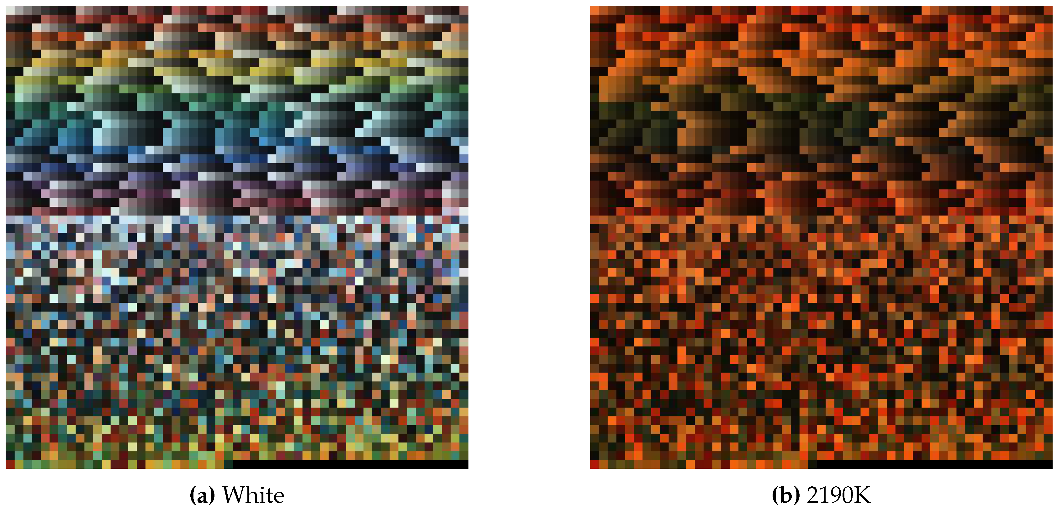
Next ten illumination spectra with temperatures (in kelvins) between 2000 K and 9000 K (sampled in equal distances in the inverse temperature, mired, scale which is more closely related to properties of human color perception) were used which resulted in the chroma values The images in Figure 1 illustrate the differences between the second image (2190 K) in the black body series and the image generated with a flat illumination spectrum.
The corresponding projections onto the unit disk (computed from the two images shown in Figure 1) are shown in Figure 2. They show that the points related to the coordinate system defining the PCA are located near the center of the disk whereas the shift of the illumination towards the red moves the corresponding points in the direction of the border of the disk.
The next figures show how the type of the statistical distributions depends on the coordinate system used. Here the ‘saturation’ data from the illuminations with temperature 2000 K and constant spectrum (, denoted by w earlier) are selected. Geometrically they are given by the radial position of the chroma points. The figures show the histograms of the two distributions and the fitted parametric distributions. In one case the radius in the unit disk is used and in the other the group-theoretically motivated hyperbolic angle is used. Three different types of parametric distributions are used: normal distributions, generalized extreme value distributions (GEV) and the Beta distribution. Figure 3a shows the fitting of the distribution of the variables computed from the 2000 K blackbody radiator. It can be seen that the data is almost normally distributed with a slight upper tail which results in a better fit by the GEV. Figure 3b shows that the white illumination source produced a distribution mainly concentrated around the origin.
The general picture is the same for the data parametrized by the radius. This is illustrated in Figure 4. Again the 2000 K radiator generates a symmetrical distribution around the mean with good fittings of the normal and the GEV distributions. The white illumination has the same characteristic as in the hyperbolic parametrization. The difference here is that, by definition the output values are located in the unit interval. For such data the Beta-distribution is a popular statistical model and we see that this gives a good fitting for both cases.
From Equation (9) it can be seen that in the case where the angle has the value zero (both points have the same angular value) the ALFs are zero for . This case will be illustrated next. From Equation (16) follows that . The value of is given by the ALF and the values are given by the MFT of the kernel. The definition of the ALFs given in Equation (9) is not suitable for numerical computations. Instead the connection between the conical functions and the Gauss hypergeometric function are often used (see [13] and the references mentioned there). In the following experiments the implementations of special functions in Mathematica were used and the numerical results exported to Matlab. In this process two problems have to be solved: (a) the integrals related to the coefficients from Equation (16) have to be calculated and (b) the discrete values in the -domain have to be selected.
For a few kernel functions k the MFT is known analytically but in the general case the integrals have to be computed numerically. In the experiments described here we used a two-stage procedure. First we selected a few relevant values in the -domain and for a given kernel k we computed the numerical values of the transform using the NIntegrate function in Mathematica using standard parameter settings. This is rather time-consuming and in the second stage of the process we therefore selected a grid on the relevant interval on the -axis and estimated the integral values by simple addition in Matlab. The grid points were chosen such that the Matlab and the Mathematica results were comparable. The result is a matrix whose entries are the values . Note that this matrix only has to be computed once. An investigation of the numerical computation of these values (comparable to the work reported in [14]) lies outside the scope of this report. Also the -grid points where selected in an ad-hoc fashion and their importance was judged afterwards.
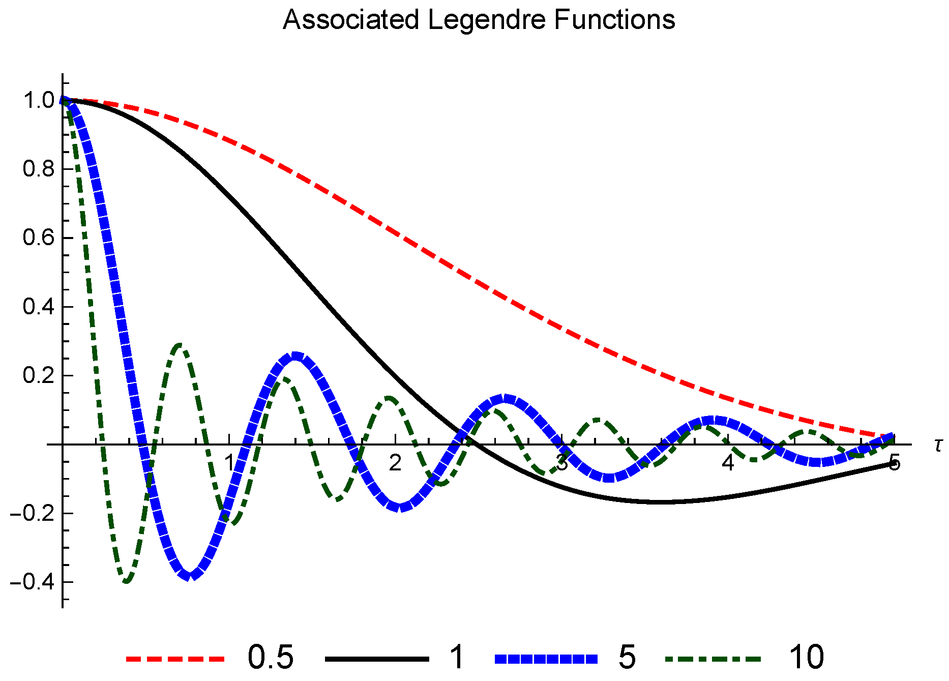
Figure 5 shows some of the ALFs in the relevant interval.
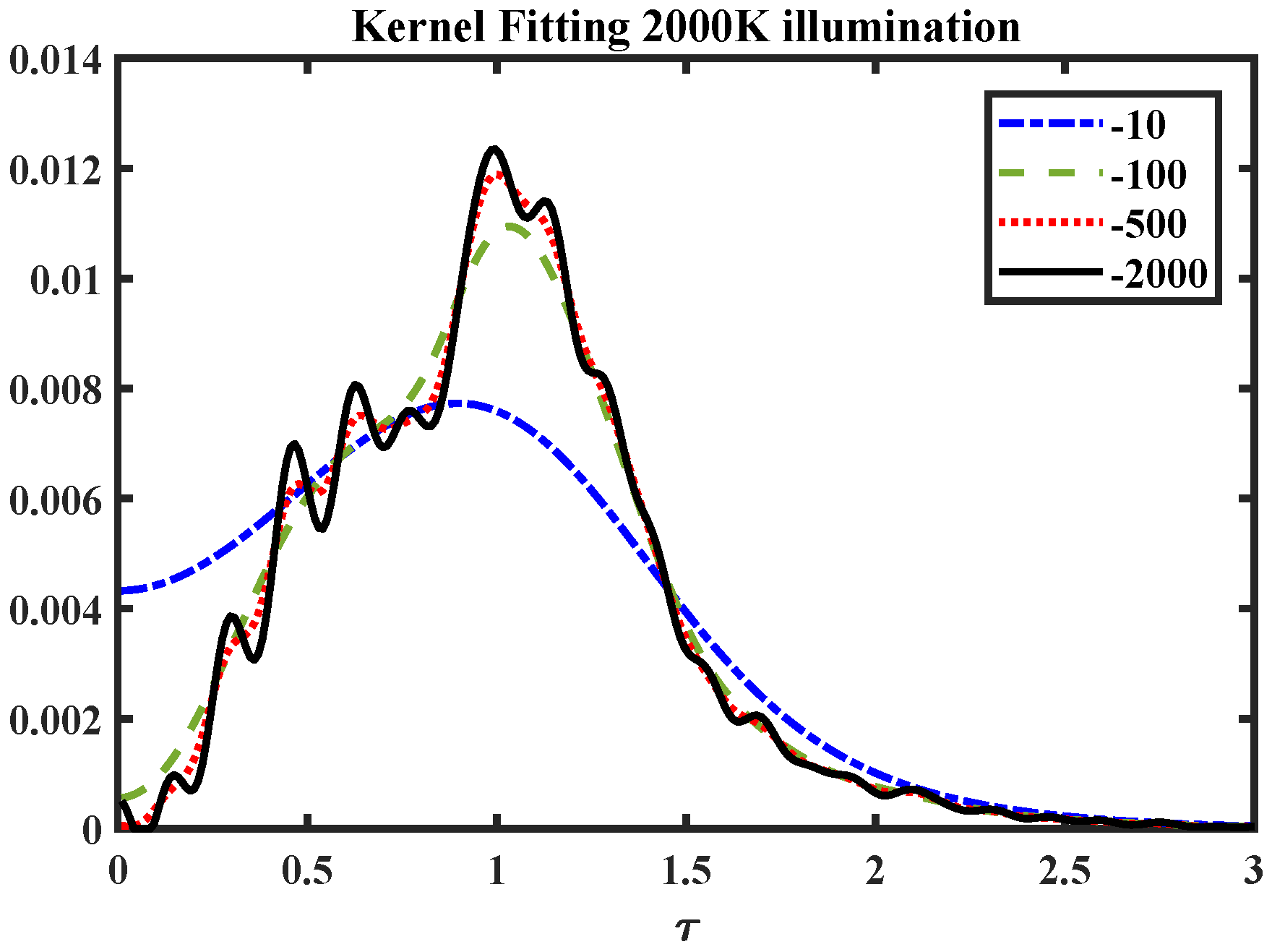
The values of the coefficients are given by the MFT of the kernel. For every kernel they have to be computed only once. This can be done by some type of numerical integration (which has to take into account the oscillatory nature of the ALFs) or one can use a kernel for which an closed expression of the MFT is available. In the following illustrations kernels of the form are used.
The width of the kernel acts as a smoothing parameter. The effect of varying the exponent of the cosh-kernel is illustrated in Figure 6. The data used are the radial values (in the parametrization) computed from the simulated images under the 2000 K illuminant. It shows that for broad kernels some general characteristics can be obtained, whereas for very thin kernels the overall estimate starts to be sensitive to small local variations.
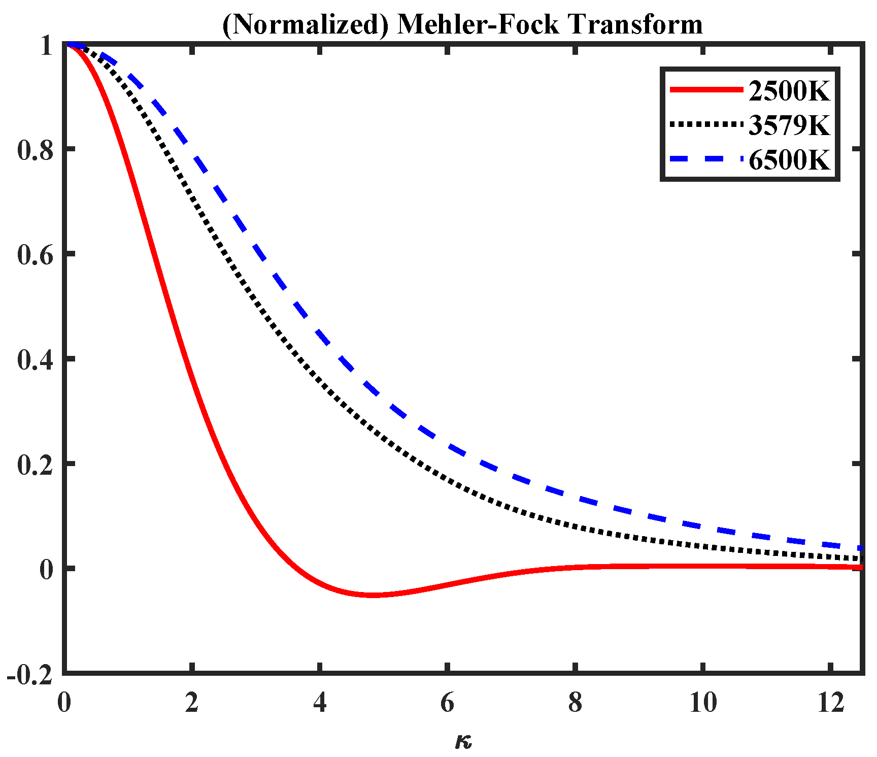
Figure 7 shows a section of the Mehler-Fock transform () for three selected illuminants. This shows how the general shift to the border of the unit disk (for the red-shifted illuminants of lower temperature) changes the form of the Mehler-Fock transform.
6. Summary and Discussion
The first part of the paper shows how projection operators lead to the unit disk as a natural domain for signals relevant in applications. The simplest example was the decomposition of a three-parameter color space into intensity, saturation and hue descriptors where the saturation/hue part is located in the unit disk. Combining the Perron-Frobenius theorem with principal component analysis showed that similar parametrizations are natural for general spaces of positive signals. Next the group was selected as a symmetry group of the unit disk. Decomposition of functions defined on domains that possess a symmetry group is studied in the theory of group representations. The group is a non-commutative and non-compact group which makes the analysis rather complicated but in exchange the class of possible transformations is much larger than an analysis based on a geometry consisting of concentric rings. It is known that the most difficult part of the theory is the analysis of the radial part of functions on the unit disk. This leads to the Mehler-Fock transform based on the ALFs. Some properties of the Mehler Fock transform were illustrated by studying the illumination-induced chroma changes in the RGB images of chips in a color atlas. Also some basic problems in the numerical implementation of the transform were discussed.
The goal of this paper was thus to introduce the relatively unknown (in the signal processing community) Mehler Fock transform and to sketch some possible application areas. Due to limited length of the text a number of interesting topics have been mentioned very briefly or not at all. These should be studied in future investigations. Some of these topics are the following:
- Study of general functions defined on the whole disc and not only functions with no angular variation. The underlying theoretical tools are combination of the transform described here with expansions in Fourier series in the angular variable. The same holds for general functions on the group which requires the application of Fourier series in the third KAK coordinate. Generalizations to the case of spaces with higher-dimensional unit balls instead of the unit disc are also well-studied in the mathematical and theoretical literature. They involve the groups SU(1,N) and their representations.
- Efficient numerical implementations and the study of numerical precisions. The transform is an integral transform and the effects of sampling and truncation decisions has to be investigated in detail.
- The separation of the data and the kernel properties was used as the main argument in favor of the transform. Not mentioned were other advantages of the combination of kernel density estimators and harmonic analysis. These are obtained from the fact that the MFT provides a decomposition of the probability density function into a superposition of ALFs. Operations, such as differentiations, on the pdf are therefore reduced to corresponding operations on the ALFS for which a large number of properties, like recursion formulas derivatives and integrals are known. Details can be found in [5,15].
Acknowledgments
The support of the Swedish Research Council through a framework grant for the project Energy Minimization for Computational Cameras (2014-6227) is gratefully acknowledged.
Conflicts of Interest
The author declares no conflict of interest.
References
- Lenz, R. Spectral Color Spaces: Their Structure and Transformations. Adv. Imaging Electron Phys. 2005, 138, 1–67. [Google Scholar]
- Lenz, R. Lie methods for color robot vision. Robotica 2008, 26, 453–464. [Google Scholar] [CrossRef]
- Hastie, T.; Tibshirani, R.; Friedman, J. The Elements of Statistical Learning: Data Mining, Inference, and Prediction; Springer Series in Statistics; Springer: New York, NY, USA, 2013. [Google Scholar]
- Said, S.; Bombrun, L.; Berthoumieu, Y.; Manton, J.H. Riemannian Gaussian distributions on the space of symmetric positive definite matrices. IEEE Trans. Inf. Theory 2017, 63, 2153–2170. [Google Scholar] [CrossRef]
- Vilenkin, N.; Klimyk, A. Representation of Lie Groups and Special Functions: Volume 1: Simplest Lie Groups, Special Functions and Integral Transforms; Springer: New York, NY, USA, 2012. [Google Scholar]
- Sneddon, I.N. The Use of Integral Transforms; McGraw-Hill: New York, NY, USA, 1972. [Google Scholar]
- Terras, A. Harmonic Analysis on Symmetric Spaces and Applications I; Springer: New York, NY, USA, 1985. [Google Scholar]
- Lebedev, N.N. Special Functions and Their Applications; Dover: New York, NY, USA, 1972. [Google Scholar]
- Bateman, H.; Erdélyi, A.; States, U. Tables of Integral Transforms; McGraw-Hill: New York, NY, USA, 1954; Volume 2. [Google Scholar]
- Wyszecki, G.; Stiles, W.S. Color Science; Wiley: New York, NY, USA, 1982. [Google Scholar]
- Parkkinen, J.P.; Hallikainen, J.; Jaaskelainen, T. Characteristic spectra of Munsell colors. J. Opt. Soc. Am. A Opt. Image Sci. Vis. 1989, 6, 318–322. [Google Scholar] [CrossRef]
- Darrodi, M.M.; Finlayson, G.; Goodman, T.; Mackiewicz, M. Reference data set for camera spectral sensitivity estimation. J. Opt. Soc. Am. A Opt. Image Sci. Vis. 2015, 32, 381–391. [Google Scholar] [CrossRef] [PubMed]
- Gil, A.; Segura, J.; Temme, N.M. Computing the Conical Function . SIAM J. Sci. Comput. 2009, 31, 1716–1741. [Google Scholar] [CrossRef]
- Gautschi, W. Computing the Kontorovich-Lebedev integral transforms and their inverses. BIT Numer. Math. 2006, 46, 21–40. [Google Scholar] [CrossRef]
- NIST Digital Library of Mathematical Functions. NIST Handbook of Mathematical Functions Hardback and CD-ROM; Olver, F.W.J., Olde Daalhuis, A.B., Lozier, D.W., Schneider, B.I., Boisvert, R.F., Clark, C.W., Miller, B.R., Saunders, B.V., Eds.; Cambridge University Press: Cambridge, UK, 2010. [Google Scholar]
Figure 1.
Simulated RGB Images. (a) White; (b) 2190 K.

Figure 2.
Chroma Points. (a) White; (b) 2190 K.
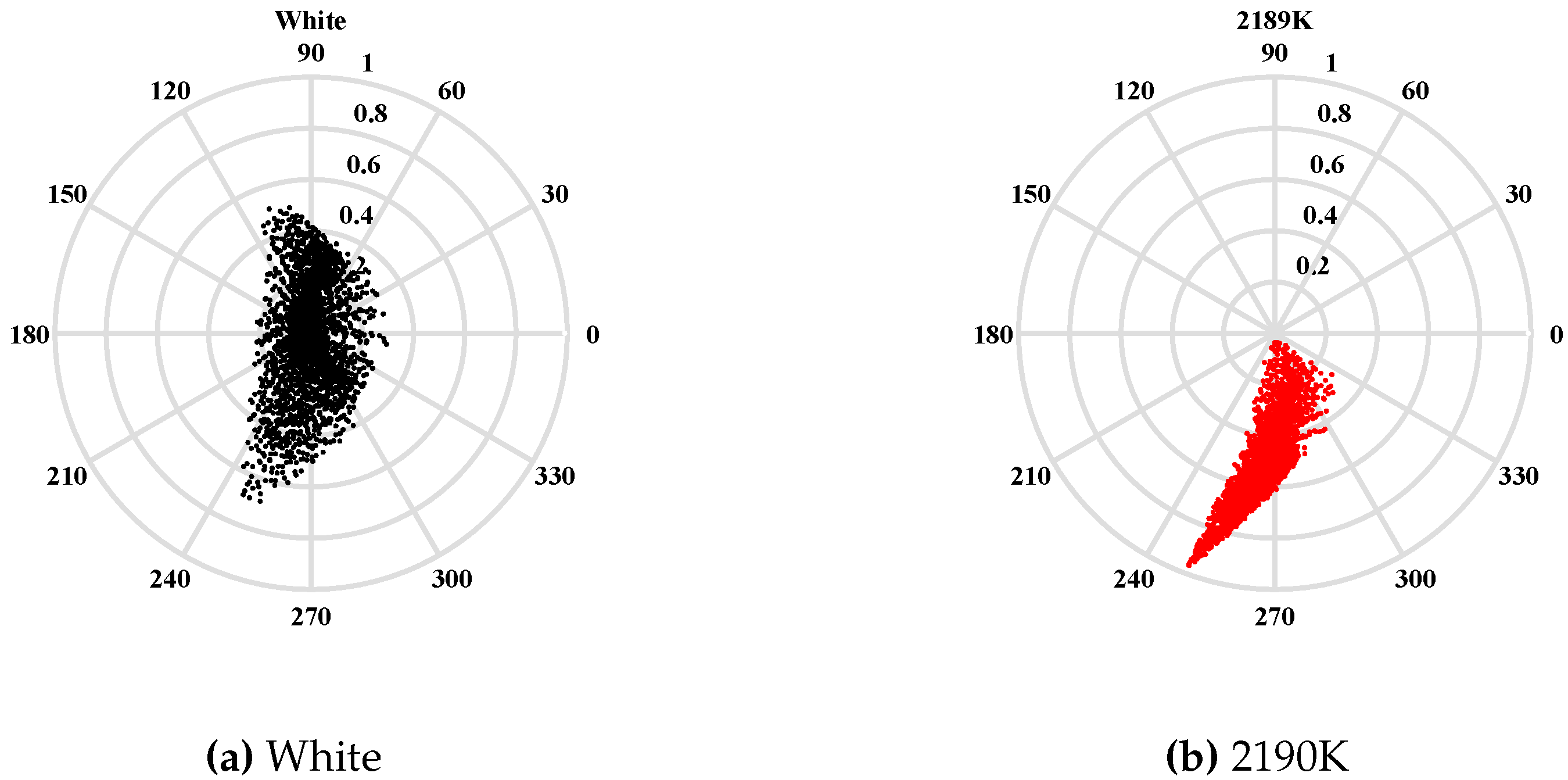
Figure 3.
-Parametrization. (a) 2000 K/-Variable/Parametric Fits; (b) White/-Variable/Parametric Fits.
Figure 3.
-Parametrization. (a) 2000 K/-Variable/Parametric Fits; (b) White/-Variable/Parametric Fits.
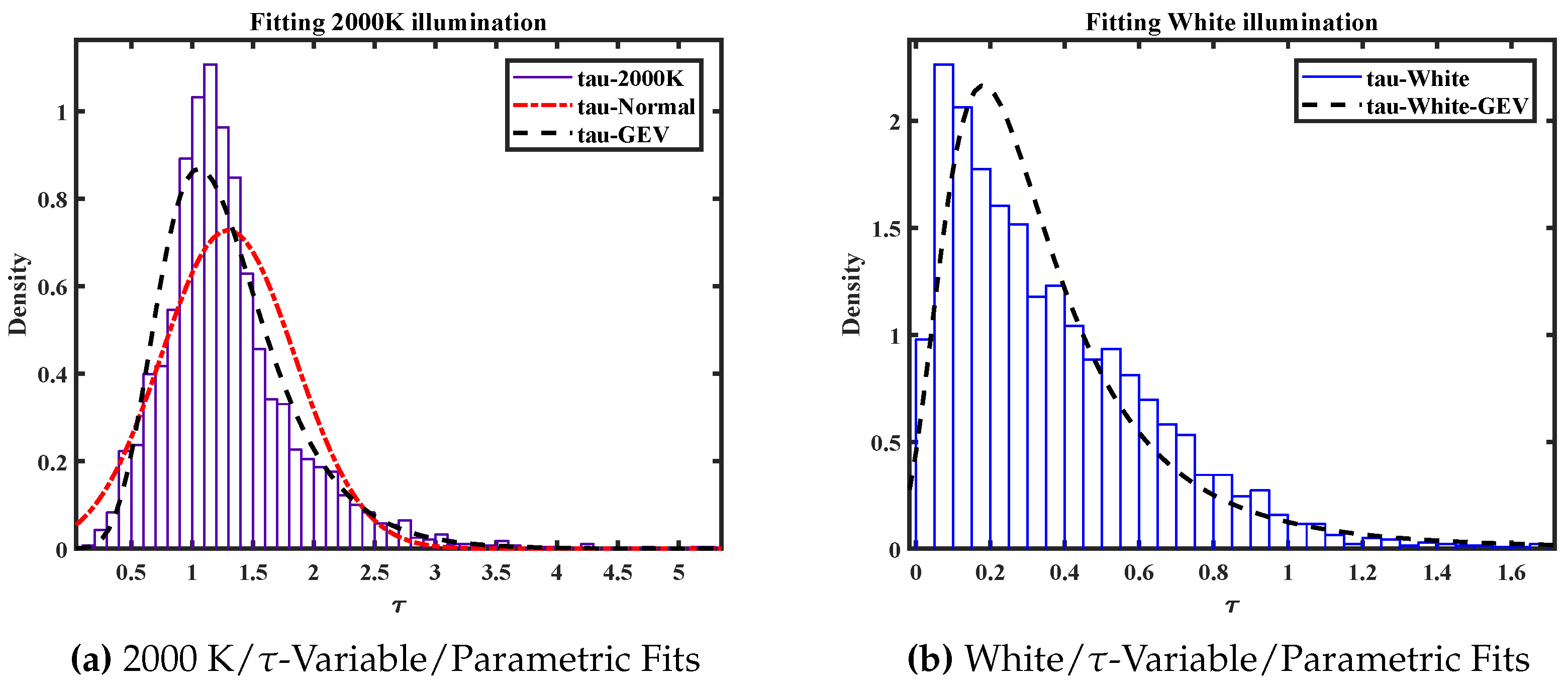
Figure 4.
-Parametrization. (a) 2000 K/-Variable/Parametric Fits; (b) White/-Variable/Parametric Fits.
Figure 4.
-Parametrization. (a) 2000 K/-Variable/Parametric Fits; (b) White/-Variable/Parametric Fits.
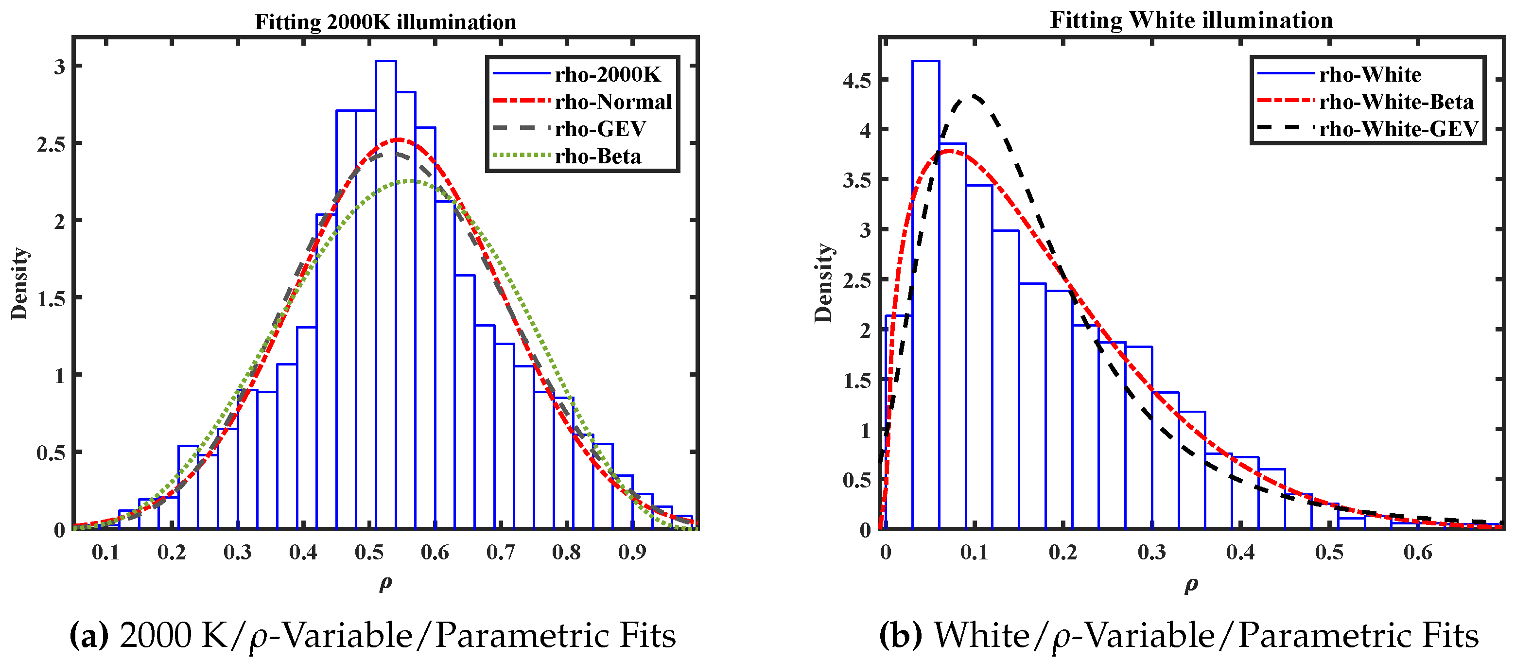
Figure 5.
Associated Legendre Functions.

Figure 6.
Kernels of varying sizes.

Figure 7.
(Normalized) Mehler-Fock-Transform.

© 2017 by the author. Licensee MDPI, Basel, Switzerland. This article is an open access article distributed under the terms and conditions of the Creative Commons Attribution (CC BY) license (http://creativecommons.org/licenses/by/4.0/).
Share and Cite
MDPI and ACS Style
Lenz, R. The Mehler-Fock Transform in Signal Processing. Entropy 2017, 19, 289. https://doi.org/10.3390/e19060289
AMA Style
Lenz R. The Mehler-Fock Transform in Signal Processing. Entropy. 2017; 19(6):289. https://doi.org/10.3390/e19060289
Chicago/Turabian StyleLenz, Reiner. 2017. "The Mehler-Fock Transform in Signal Processing" Entropy 19, no. 6: 289. https://doi.org/10.3390/e19060289
Note that from the first issue of 2016, this journal uses article numbers instead of page numbers. See further details here.