Analytical Approximate Solutions of (n + 1)-Dimensional Fractal Heat-Like and Wave-Like Equations


1
Department of Mathematics, Faculty of Art and Science, Siirt University, Siirt 56100, Turkey
2
Department of Mathematics, Faculty of Art and Sciences, Çankaya University, Ankara 06790, Turkey
3
Institute of Space Sciences, Magurele-Bucharest 077125, Romania
4
Department of Mathematics, Faculty of Art and Science, King Saud University, Riyadh 11495, Saudi Arabia
5
Department of Mathematics, Faculty of Science, Yuzuncu Yil University, Van 65080, Turkey
*
Author to whom correspondence should be addressed.
Entropy 2017, 19(7), 296; https://doi.org/10.3390/e19070296
Submission received: 27 May 2017
/
Revised: 15 June 2017
/
Accepted: 20 June 2017
/
Published: 22 June 2017
(This article belongs to the Special Issue Complex Systems and Fractional Dynamics)
Abstract
:In this paper, we propose a new type (n + 1)-dimensional reduced differential transform method (RDTM) based on a local fractional derivative (LFD) to solve (n + 1)-dimensional local fractional partial differential equations (PDEs) in Cantor sets. The presented method is named the (n + 1)-dimensional local fractional reduced differential transform method (LFRDTM). First the theories, their proofs and also some basic properties of this procedure are given. To understand the introduced method clearly, we apply it on the (n + 1)-dimensional fractal heat-like equations (HLEs) and wave-like equations (WLEs). The applications show that this new technique is efficient, simply applicable and has powerful effects in (n + 1)-dimensional local fractional problems.
1. Introduction
The importance of fractional calculus and its popularity have increased during the past four decades, due to its applications in many fields of engineering and applied science. For example, analysis of entropy in fractional dynamical systems, entropy in thermodynamics, control theory of dynamic systems, probability and statistics, electrical networks, signal processing, optics, chemical physics, the electrochemistry of corrosion and so on can all be successfully modelled by fractional order differential equations [1,2,3,4,5,6,7,8,9,10,11,12,13,14,15,16,17,18,19,20,21,22,23,24,25,26,27,28,29,30,31,32,33,34,35,36,37,38,39].
In thermodynamics, entropy is known as a state function of a thermodynamic system. The production of entropy by fractional calculus was suggested in [4]. The production of entropy rate for fractional diffusion processes was discussed in [6,7,8]. The analysis of entropy in fractional dynamic systems was proposed in [10]. However, these entropy processes are differentiable. Non-differentiable production of entropy in heat conduction of the fractal temperature field was studied in [13]. The heat conduction equation was discussed by the help of local fractional derivative (LFD) [26]. Some numerical methods are applied to many non-differentiable problems in Cantor sets by using LFD [21,22,23,24,25,26,27,28,29].
The differential transform method (DTM) which is constructed based on Taylor expansion has been a widely used approximation method in recent years. The DTM was introduced and applied to engineering problems by Zhou [40]. The method was applied to solve linear, nonlinear, ordinary, partial and fractional order differential equation problems in biology, engineering, physics [41,42,43,44,45,46,47,48,49] and so on. The reduced differential transform method (RDTM) was presented by Keskin and Oturanc [50,51,52] to simplify the DTM calculations. The method is a reliable semi-analytical approach used to find solutions of many types of linear, non-linear, fractional non-fractional order partial differential equations (PDEs). There have been many application of RDTM [50,51,52,53,54,55,56,57,58,59,60]. Previously, the use of LFD with DTM and RDTM was introduced as local fractional DTM (LFDTM) [27] and local fractional reduced differential transform method (LFRDTM) [28]. Furthermore, some basic theorems and applications were given for these methods [27,28]. In addition to that, we now introduce the (n + 1)-dimensional case of RDTM with LFD for the first time. The basic definitions and theorems of (n + 1)-dimensional LFRDTM are given. Moreover, the presented method was applied to both (n + 1)-dimensional fractal homogeneous and inhomogeneous HLEs and WLEs. These equations have been studied by many researchers [60,61,62,63,64]. However, in fractal space, these problems are discussed using (n + 1)-dimensional LFRDTM for the first time.
In our present study, the basic definitions of local fractional calculus are given in Section 2. Two-dimensional LFRDTM and (n + 1)-dimensional LFRDTM with the basic definitions and theorems are presented in Section 3. In Section 4, the applications of the new method, graphics of the solutions and discussion are given and finally, we put forth our conclusions in Section 5.
2. Preliminaries
In this section, we give same basic definitions and important properties of LFD on fractal space [11,27].
Definition 1.
Let be a set of the non-differentiable functions with the fractal dimension . For the LFD operator of of order at the is defined as follows [11]:
where:
Lemma 1
- (i)
- for ,
- (ii)
- ,
- (iii)
- .
Definition 2.
3. Main Results
In this section, we describe two-dimensional LFRDTM and (n + 1)-dimensional LFRDTM.
3.1. Two-Dimensional LFRDTM
In this subsection, we recall and review briefly the local fractional Taylor theorems, and then, we extend two-dimensional LFRDTM.
Definition 3.
Definition 4.
Using Definitions 3 and 4, Based on results of [28], the fundamental mathematical operations of the two-dimensional LFRDTM are presented in Table 2:
In Table 2, the lowercase , and represent the local fractional analytic original functions while the uppercase , and stand for LFRDT functions. and are constants.
3.2. (n + 1)-Dimensional LFRDTM
In this subsection, the lowercase represents the local fractional analytic original function while the uppercase stands for (n + 1)-dimensional LFRDT function. Here is used for through the study. The basic definitions of (n + 1)-dimensional LFRDTM are presented as follows.
Definition 5.
The (n + 1)-dimensional LFRDT of the function is defined by the following formula:
where and
Definition 6.
The (n + 1)-dimensional local fractional reduced differential inverse transform of is defined by the following formula:
where
Using Definitions 5 and 6, the theorems of (n + 1)-dimensional LFRDTM, which is the more general form of the operations given in Table 2, are deduced as follows:
Theorem 1.
Let and be constants. If then .
Proof.
(n + 1)-dimensional LFRDT of and can be written as the following:
From (12), is obtained as:
The proof is thus completed. ☐
Theorem 2.
If , then .
Proof.
By the help of Definition 6, and can be written that:
Then, from (14), is obtained as:
Hence, is found as:
The proof is thus completed. ☐
Theorem 3.
If , then .
Proof.
By the help of Definition 6, (n + 1)-dimensional LFRDT of can be written that:
For , by using (17), can be obtained as:
The proof is thus completed. ☐
Theorem 4.
If , then , where
Proof.
From Definition 5, we have:
The proof is thus completed. ☐
4. Applications of (n + 1)-Dimensional LFRDTM
Example 1.
Firstly, we consider (2 + 1)-dimensional local fractional homogeneous HLE on a Cantor set:
with the initial condition (IC):
where .
Now solve this problem by using (n + 1)-dimensional LFRDTM. By taking the (n + 1)-dimensional LFRDT of (20), it can be obtained that:
The (n + 1)-dimensional LFRDT of the IC in (21) is given by:
By using (23) in (22), we can obtain the following values successively:
From (24), the values give the following approximation solution:
Hence, from (25), is:
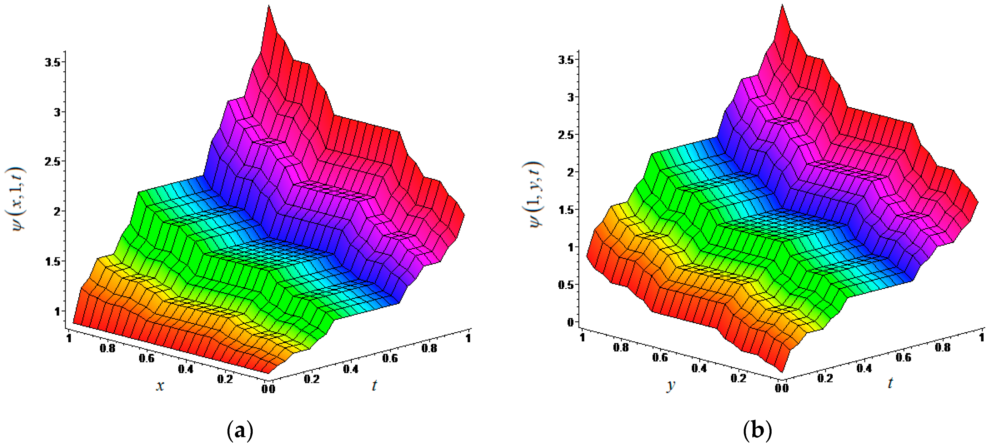
This finding is the exact solution of the (2 + 1)-dimensional local fractional homogeneous HLE (20) on the Cantor set. The graph of this solution is given in Figure 1 for .
Example 2.
Secondly, consider the following (3 + 1)-dimensional local fractional inhomogeneous HLE on a Cantor set:
subject to the IC:
here and
Using (n + 1)-dimensional LFRDTM, Equation (27) transforms to:
From the IC (28), we write:
From (30) and (29), the following values can be obtained:
From (31), the following approximation solution can be written as:
Hence, from (32), is:
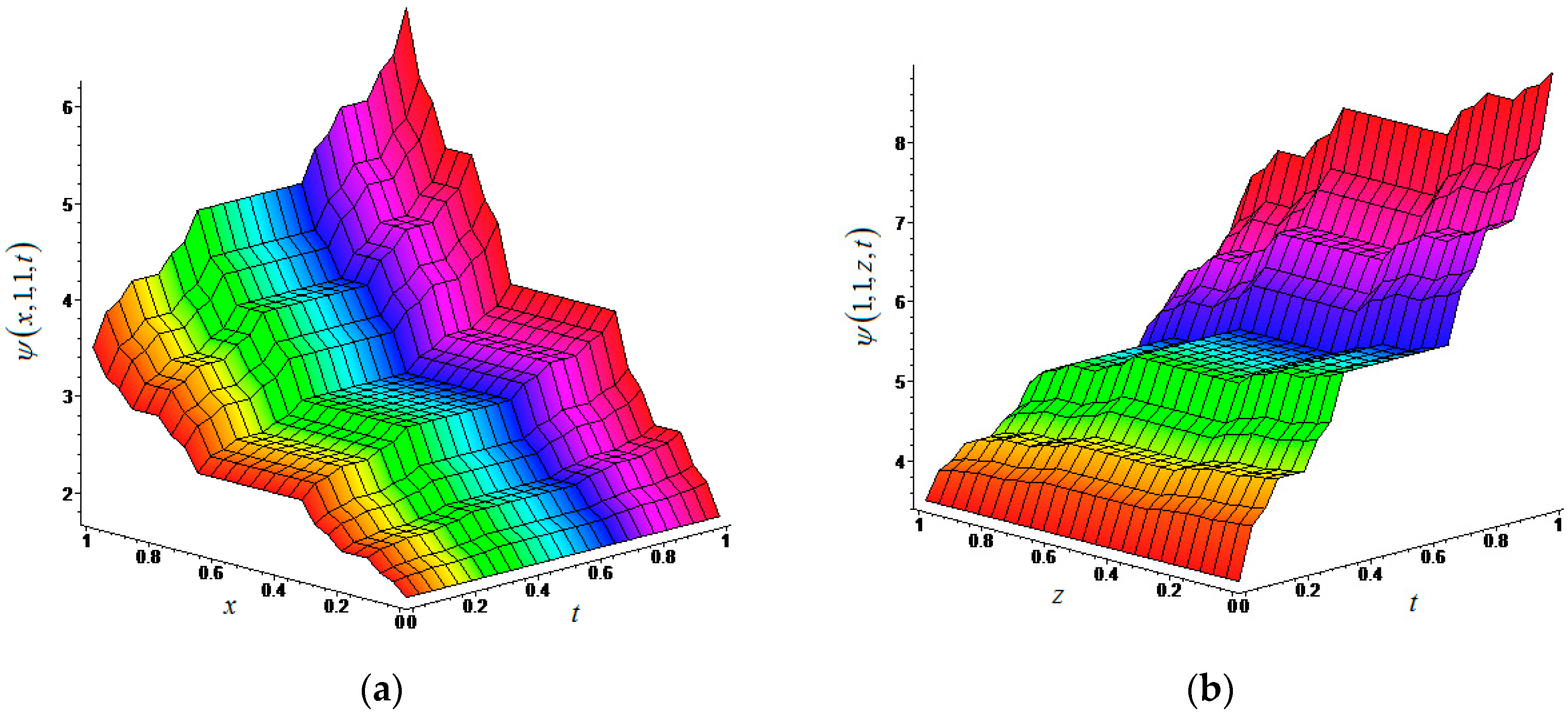
This result is the exact solution of the (3 + 1)-dimensional local fractional inhomogeneous HLE (27) on the Cantor set. The graph of this solution is given in Figure 2 for α = ln2/ln3.
Example 3.
Thirdly, we consider (2 + 1)-dimensional local fractional homogeneous WLE on a Cantor set:
with the ICs:
here
We solve this problem by using (n + 1)-dimensional LFRDTM. By taking (n + 1)-dimensional LFRDT of (34), it can be obtained that:
From the ICs (35), it can be written as follows:
By using (37) in (36), we can obtain the following values successively:
From (38), the values give the following approximation solution:
Hence, from (39), is:
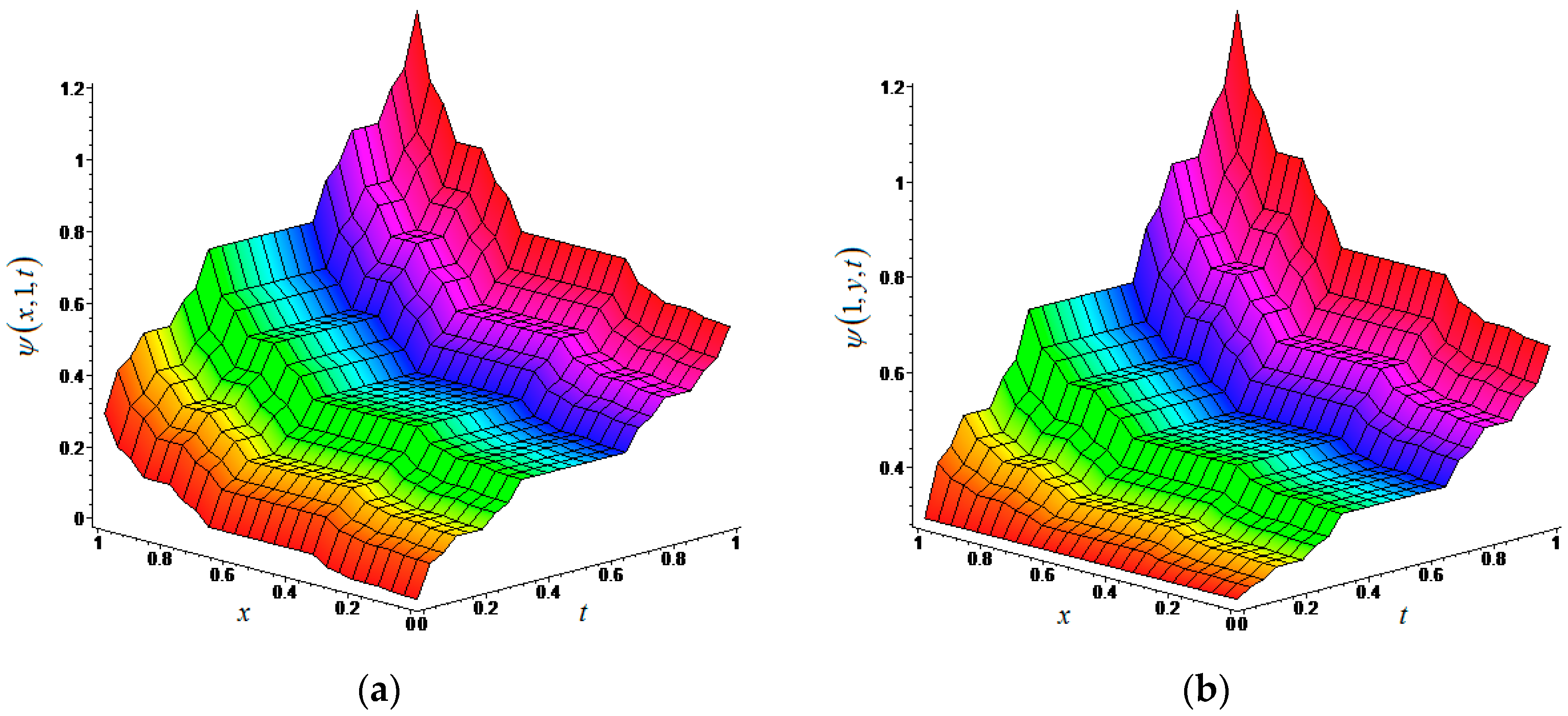
This finding is the exact solution of the (2 + 1)-dimensional local fractional homogeneous WLE (34) on the Cantor set. The graph of this solution is given in Figure 3 for α = ln2/ln3.
Example 4.
Finally, consider the (3 + 1)-dimensional local fractional inhomogeneous WLE on a Cantor set:
subject to the ICs:
where
According to (n + 1)-dimensional LFRDTM, (n + 1)-dimensional LFRDT of (41) can be written that:
From the ICs (42) we write:
According to (44) and (43), we can obtain the following values:
By using (38), the values give the following approximation solution:
Hence, from (46), is:
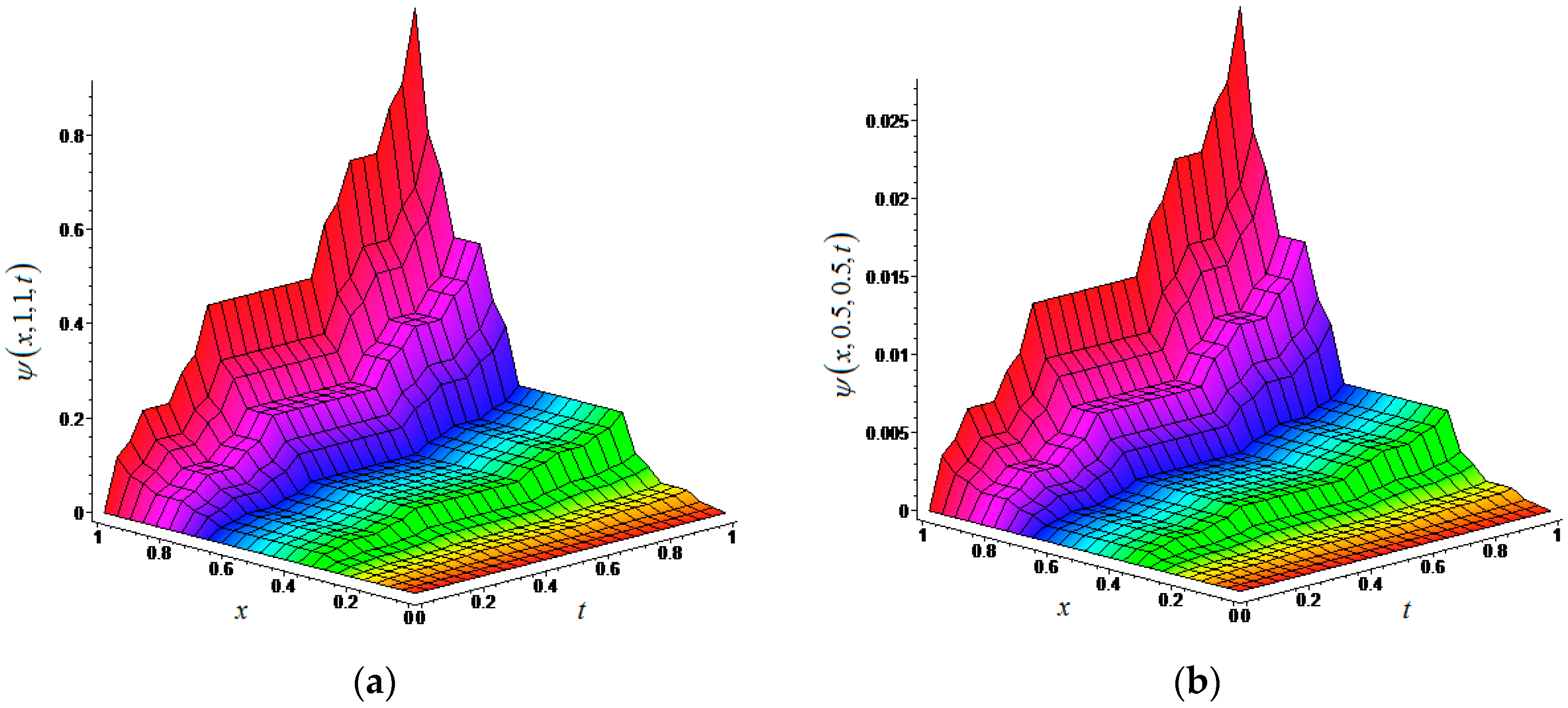
This result obtained is the exact solution of the (3 + 1)-dimensional local fractional inhomogeneous WLE (41) on Cantor set. The graph of this solution is given in Figure 4 for α = ln2/ln3.
5. Conclusions
In this paper, a new technique, (n + 1)-dimensional local fractional reduced differential transform method (LFRDTM), was presented to find the analytical approximate solutions of local fractional PDEs. Then, the new method was applied to (n + 1)-dimensional fractal HLEs and WLEs. In the applications, our method directly gave us the exact solution for the problems without any transformation, discretization and any other restrictions. Physical behaviors of the solutions on fractal spaces were illustrated using 3D graphics. The results showed that presented method gives good outcomes for solutions of (n + 1)-dimensional local fractional PDEs. Hence, our results suggest that the new procedure (n + 1)-dimensional LFRDTM is reliable, useful and simplify for local fractional PDEs to solve many complicated fractal problems.
Acknowledgments
The authors extend their appreciation to the International Scientific Partnership Program ISPP at King Saud University for funding this research work through ISPP# 63.
Author Contributions
Omer Acan wrote this manuscript. Omer Acan, Dumitru Baleanu, Maysaa Mohamed Al Qurashi and Mehmet Giyas Sakar prepared the final version of the paper and analyzed. All authors have read and approved the final manuscript.
Conflicts of Interest
The authors declare no conflict of interest.
References
- Oldham, K.; Spanier, J. The Fractional Calculus: Theory and Applications of Differentiation and Integration to Arbitary Order; Academic Press: New York, NY, USA, 1974. [Google Scholar]
- Miller, K.; Ross, B. An Introduction to the Fractional Calculus and Fractional Differential Equations; Wiley: New York, NY, USA, 1993. [Google Scholar]
- Samko, S.G.; Kilbas, A.A.; Marichev, O.I. Fractional Integrals and Derivatives; Gordon and Breach Science Publishers: Yverdon, Switzerland, 1993. [Google Scholar]
- Hoffmann, K.H.; Essex, C.; Schulzky, C. Fractional Diffusion and Entropy Production. J. Non-Equilib. Thermodyn. 1998, 23, 166–175. [Google Scholar] [CrossRef]
- Podlubny, I. Fractional Differential Equations; Academic Press: New York, NY, USA, 1999. [Google Scholar]
- Essex, C.; Schulzky, C.; Franz, A. Tsallis and Renyi entropies in fractional diffusion and entropy production. Phys. A Stat. Mech. Appl. 2000, 284, 299–308. [Google Scholar] [CrossRef]
- Li, X.; Essex, C.; Davison, M.; Hoffmann, K.H.; Schulzky, C. Fractional Diffusion, Irreversibility and Entropy. J. Non-Equilib. Thermodyn. 2003, 28, 279–291. [Google Scholar] [CrossRef]
- Magin, R.L.; Ingo, C. Entropy and Information in a Fractional Order Model of Anomalous Diffusion. IFAC Proc. Vol. 2012, 45, 428–433. [Google Scholar] [CrossRef]
- Sabatier, J.; Agrawal, O.P.; Machado, J.A.T. Advances in Fractional Calculus; Springer: Dordrecht, The Netherlands, 2007. [Google Scholar]
- Machado, J.A.T. Entropy analysis of integer and fractional dynamical systems. Nonlinear Dyn. 2010, 62, 371–378. [Google Scholar]
- Yang, X.J. Advanced Local Fractional Calculus and Its Applications; World Science: New York, NY, USA, 2012. [Google Scholar]
- He, J.H. A Tutorial Review on Fractal Spacetime and Fractional Calculus. Int. J. Theor. Phys. 2014, 53, 3698–3718. [Google Scholar] [CrossRef]
- Zhang, Y.; Baleanu, D.; Yang, X. On a Local Fractional Wave Equation under Fixed Entropy Arising in Fractal Hydrodynamics. Entropy 2014, 16, 6254–6262. [Google Scholar] [CrossRef]
- Baleanu, D.; Khan, H.; Jafari, H.; Khan, R.A. On the exact solution of wave equations on cantor sets. Entropy 2015, 17, 6229–6237. [Google Scholar] [CrossRef]
- Rogosin, S. The Role of the Mittag-Leffler Function in Fractional Modeling. Mathematics 2015, 3, 368–381. [Google Scholar]
- Salahshour, S.; Ahmadian, A.; Senu, N.; Baleanu, D.; Agarwal, P. On analytical solutions of the fractional differential equation with uncertainty: Application to the basset problem. Entropy 2015, 17, 885–902. [Google Scholar] [CrossRef]
- Yang, X.J.; Baleanu, D.; Srivastava, H.M. Local fractional similarity solution for the diffusion equation defined on Cantor sets. Appl. Math. Lett. 2015, 47, 54–60. [Google Scholar] [CrossRef]
- Ahmad, J.; Mohyud-din, S.T. Solving Wave and Diffusion Equations on Cantor Sets. Proc. Pak. Acad. Sci. 2015, 52, 81–87. [Google Scholar]
- Yang, X.J.; Machado, J.A.T.; Hristov, J. Nonlinear dynamics for local fractional Burgers’ equation arising in fractal flow. Nonlinear Dyn. 2016, 84, 3–7. [Google Scholar] [CrossRef]
- Jafari, H.; Jassim, H.; Al Qurashi, M.; Baleanu, D. On the Existence and Uniqueness of Solutions for Local Fractional Differential Equations. Entropy 2016, 18, 420. [Google Scholar] [CrossRef]
- Yang, Y.J.; Baleanu, D.; Yang, X.J. A local fractional variational iteration method for laplace equation within local fractional operators. Abstr. Appl. Anal. 2013, 2013, 202650. [Google Scholar] [CrossRef]
- Baleanu, D.; Machado, J.A.T.; Cattani, C.; Baleanu, M.C.; Yang, X.J. Local fractional variational iteration and decomposition methods for wave equation on cantor sets within local fractional operators. Abstr. Appl. Anal. 2014, 2014, 535048. [Google Scholar] [CrossRef]
- Yang, Y.J.; Hua, L.Q. Variational Iteration Transform Method for Fractional Differential Equations with Local Fractional Derivative. Abstr. Appl. Anal. 2014, 2014, 760957. [Google Scholar] [CrossRef]
- Zhang, Y.Z.; Yang, A.M.; Long, Y. Initial boundary value problem for fractal heat equation in the semi-infinite region by Yang-Laplace transform. Therm. Sci. 2014, 18, 677–681. [Google Scholar] [CrossRef]
- Yang, X.J.; Srivastava, H.M.; Cattani, C. Local fractional homotopy perturbation method for solving fractal partial differential equations arising in mathematical physics. Rom. Rep. Phys. 2015, 67, 752–761. [Google Scholar]
- Zhang, Y.; Cattani, C.; Yang, X.J. Local Fractional Homotopy Perturbation Method for Solving Non-Homogeneous Heat Conduction Equations in Fractal Domains. Entropy 2015, 17, 6753–6764. [Google Scholar] [CrossRef]
- Yang, X.J.; Machado, J.A.T.; Srivastava, H.M. A new numerical technique for solving the local fractional diffusion equation: Two-dimensional extended differential transform approach. Appl. Math. Comput. 2016, 274, 143–151. [Google Scholar] [CrossRef]
- Jafari, H.; Jassim, H.K.; Moshokoa, S.P.; Ariyan, V.M.; Tchier, F. Reduced differential transform method for partial differential equations within local fractional derivative operators. Adv. Mech. Eng. 2016, 8, 1–6. [Google Scholar] [CrossRef]
- Guo, Z.H.; Acan, O.; Kumar, S. Sumudu transform series expansion method for solving the local fractional Laplace equation in fractal thermal problems. Therm. Sci. 2016, 20, 739–742. [Google Scholar] [CrossRef]
- Liemert, A.; Kienle, A. Fractional Schrödinger Equation in the Presence of the Linear Potential. Mathematics 2016, 4, 31. [Google Scholar] [CrossRef]
- Yang, X.J.; Gao, F.; Srivastava, H.M. Exact travelling wave solutions for the local fractional two-dimensional Burgers-type equations. Comput. Math. Appl. 2017, 73, 203–210. [Google Scholar] [CrossRef]
- Yang, X.J.; Machado, J.A.T.; Cattani, C.; Gao, F. On a fractal LC-electric circuit modeled by local fractional calculus. Commun. Nonlinear Sci. Numer. Simul. 2017, 47, 200–206. [Google Scholar] [CrossRef]
- Machado, J.A.T.; Lopes, A.M. Complex and fractional dynamics. Entropy 2017, 19, 62. [Google Scholar] [CrossRef]
- Su, N. Exact and Approximate Solutions of Fractional Partial Differential Equations for Water Movement in Soils. Hydrology 2017, 4, 8. [Google Scholar] [CrossRef]
- Jassim, H.K. The analytical solutions for volterra integro-differential equations within local fractional operators by yang-laplace transform. Commun. Math. Anal. 2017, 6, 69–76. [Google Scholar]
- Yang, X.J.; Machado, J.A.T.; Nieto, J.J. A new family of the local fractional PDEs. Fundam. Inform. 2017, 151, 63–75. [Google Scholar] [CrossRef]
- Baleanu, D.; Machado, J.A.T.; Luo, A.C.J. Fractional Dynamics and Control; Springer Science & Business Media: Berlin, Germany, 2011. [Google Scholar]
- Pinto, C.M.A.; Machado, J.A.T. Fractional model for malaria transmission under control strategies. Comput. Math. Appl. 2013, 66, 908–916. [Google Scholar] [CrossRef]
- Bayour, B.; Torres, D.F.M. Existence of solution to a local fractional nonlinear differential equation. J. Comput. Appl. Math. 2017, 312, 127–133. [Google Scholar] [CrossRef]
- Zhou, J.K. Differential Transformation and its Application for Electrical Circuits; Huazhong University Press: Wuhan, China, 1986. [Google Scholar]
- Chen, C.; Ho, S. Solving partial differential equations by two-dimensional differential transform method. Appl. Math. Comput. 1999, 106, 171–179. [Google Scholar]
- Ayaz, F. On the two-dimensional differential transform method. Appl. Math. Comput. 2003, 143, 361–374. [Google Scholar] [CrossRef]
- Ayaz, F. Solutions of the system of differential equations by differential transform method. Appl. Math. Comput. 2004, 147, 547–567. [Google Scholar] [CrossRef]
- Momani, S.; Odibat, Z.; Erturk, V.S. Generalized differential transform method for solving a space- and time-fractional diffusion-wave equation. Phys. Lett. A 2007, 370, 379–387. [Google Scholar] [CrossRef]
- Ertürk, V.S.; Momani, S. Solving systems of fractional differential equations using differential transform method. J. Comput. Appl. Math. 2008, 215, 142–151. [Google Scholar] [CrossRef]
- Zedan, H.A.; Alghamdi, M.A. Solution of (3 + 1)-Dimensional Nonlinear Cubic Schrodinger Equation by Differential Transform Method. Math. Probl. Eng. 2012, 2012, 1–14. [Google Scholar] [CrossRef]
- Abuteen, E.; Momani, S.; Alawneh, A. Solving the fractional nonlinear Bloch system using the multi-step generalized differential transform method. Comput. Math. Appl. 2014, 68, 2124–2132. [Google Scholar] [CrossRef]
- Di Matteo, A.; Pirrotta, A. Generalized differential transform method for nonlinear boundary value problem of fractional order. Commun. Nonlinear Sci. Numer. Simul. 2015, 29, 88–101. [Google Scholar] [CrossRef]
- Kurnaz, A.; Oturanc, G.; Kiris, M.E. n-Dimensional differential transformation method for solving PDEs. Int. J. Comput. Math. 2005, 82, 369–380. [Google Scholar] [CrossRef]
- Keskin, Y.; Oturanc, G. Reduced differential transform method for partial differential equations. Int. J. Nonlinear Sci. Numer. Simul. 2009, 10, 741–749. [Google Scholar] [CrossRef]
- Keskin, Y.; Oturanc, G. The reduced differential transform method: A new approach to factional partial differential equations. Nonlinear Sci. Lett. A 2010, 1, 207–217. [Google Scholar]
- Keskin, Y.; Oturanc, G. Reduced Differential Transform Method for Generalized KdV Equations. Math. Comput. Appl. 2010, 15, 382–393. [Google Scholar] [CrossRef]
- Saha Ray, S. Numerical solutions and solitary wave solutions of fractional KDV equations using modified fractional reduced differential transform method. Comput. Math. Math. Phys. 2013, 53, 1870–1881. [Google Scholar] [CrossRef]
- Acan, O.; Keskin, Y. Reduced differential transform method for (2 + 1) dimensional type of the Zakharov–Kuznetsov ZK(n,n) equations. In Proceedings of the 12th International Conference of Numerical Analysis and Applied Mathematics (ICNAAM-2014), Rhodes, Greece, 22–28 September 2014. [Google Scholar]
- Acan, O.; Keskin, Y. Approximate solution of Kuramoto–Sivashinsky equation using reduced differential transform method. In Proceedings of the 12th International Conference of Numerical Analysis and Applied Mathematics (ICNAAM-2014), Rhodes, Greece, 22–28 September 2014. [Google Scholar]
- Acan, O.; Keskin, Y. A new technique of Laplace Pade reduced differential transform method for (1 + 3) dimensional wave equations. New Trends Math. Sci. 2017, 5, 164–171. [Google Scholar] [CrossRef]
- Acan, O.; Keskin, Y. A Comparative Study of Numerical Methods for Solving (n + 1) Dimensional and Third-Order Partial Differential Equations. J. Comput. Theor. Nanosci. 2016, 13, 8800–8807. [Google Scholar] [CrossRef]
- Acan, O.; Firat, O.; Keskin, Y.; Oturanc, G. Solution of Conformable Fractional Partial Differential Equations by Reduced Differential Transform Method. Selcuk J. Appl. Math. 2016, in press. [Google Scholar]
- Acan, O.; Firat, O.; Keskin, Y. The Use of Conformable Variational Iteration Method, Conformable Reduced Differential Transform Method and Conformable Homotopy Analaysis Method for Solving Different Types of Nonlinear Partial Differential Equations. In Proceedings of the 3rd International Conference on Recent Advances in Pure and Applied Mathematics, Bodrum, Turkey, 19–23 May 2016. [Google Scholar]
- Wazwaz, A.M.; Gorguis, A. Exact solutions for heat-like and wave-like equations with variable coefficients. Appl. Math. Comput. 2004, 149, 15–29. [Google Scholar] [CrossRef]
- Momani, S. Analytical approximate solution for fractional heat-like and wave-like equations with variable coefficients using the decomposition method. Appl. Math. Comput. 2005, 165, 459–472. [Google Scholar] [CrossRef]
- Molliq, R.Y.; Noorani, M.S.M.; Hashim, I. Variational iteration method for fractional heat- and wave-like equations. Nonlinear Anal. Real World Appl. 2009, 10, 1854–1869. [Google Scholar] [CrossRef]
- Zhang, S.; Zhu, R.; Zhang, L. Exact solutions of fractional heat-like and wave-like equations with variable coefficients. Therm. Sci. 2016, 20, 689–693. [Google Scholar] [CrossRef]
- Avcı, D.; İskender Eroğlu, B.B.; Özdemir, N. Conformable Fractional Wave-Like Equation on a Radial Symmetric Plate; Springer International Publishing: New York, NY, USA, 2017; pp. 137–146. [Google Scholar]
Figure 1.
(a) The exact solution of (2 + 1)-dimensional local fractional homogeneous HLE (20) in fractal space for with α = ln2/ln3; (b) The exact solution of (2 + 1)-dimensional local fractional homogeneous HLE (20) in fractal space for with α = ln2/ln3.
Figure 1.
(a) The exact solution of (2 + 1)-dimensional local fractional homogeneous HLE (20) in fractal space for with α = ln2/ln3; (b) The exact solution of (2 + 1)-dimensional local fractional homogeneous HLE (20) in fractal space for with α = ln2/ln3.

Figure 2.
(a) The exact solution of (3 + 1)-dimensional local fractional inhomogeneous HLE (27) in fractal space for with α = ln2/ln3; (b) The exact solution of (3 + 1)-dimensional local fractional inhomogeneous HLE (27) in fractal space for with α = ln2/ln3.
Figure 2.
(a) The exact solution of (3 + 1)-dimensional local fractional inhomogeneous HLE (27) in fractal space for with α = ln2/ln3; (b) The exact solution of (3 + 1)-dimensional local fractional inhomogeneous HLE (27) in fractal space for with α = ln2/ln3.

Figure 3.
(a) The exact solution of (2 + 1)-dimensional local fractional homogeneous WLE (34) in fractal space for with α = ln2/ln3; (b) The exact solution of (2 + 1)-dimensional local fractional homogeneous WLE (34) in fractal space for with α = ln2/ln3.
Figure 3.
(a) The exact solution of (2 + 1)-dimensional local fractional homogeneous WLE (34) in fractal space for with α = ln2/ln3; (b) The exact solution of (2 + 1)-dimensional local fractional homogeneous WLE (34) in fractal space for with α = ln2/ln3.

Figure 4.
(a) The exact solution of (3 + 1)-dimensional local fractional inhomogeneous WLE (41) in fractal space for with α = ln2/ln3; (b) The exact solution of (3 + 1)-dimensional local fractional inhomogeneous WLE (41) in fractal space for with α = ln2/ln3.
Figure 4.
(a) The exact solution of (3 + 1)-dimensional local fractional inhomogeneous WLE (41) in fractal space for with α = ln2/ln3; (b) The exact solution of (3 + 1)-dimensional local fractional inhomogeneous WLE (41) in fractal space for with α = ln2/ln3.

Table 1.
The some basic operations of LFD.
| Special Functions | ||
|---|---|---|
Table 2.
Basic operations of the two-dimensional LFRDTM.
| Original Function | Transformed Function |
|---|---|
© 2017 by the authors. Licensee MDPI, Basel, Switzerland. This article is an open access article distributed under the terms and conditions of the Creative Commons Attribution (CC BY) license (http://creativecommons.org/licenses/by/4.0/).
Share and Cite
MDPI and ACS Style
Acan, O.; Baleanu, D.; Qurashi, M.M.A.; Sakar, M.G. Analytical Approximate Solutions of (n + 1)-Dimensional Fractal Heat-Like and Wave-Like Equations. Entropy 2017, 19, 296. https://doi.org/10.3390/e19070296
AMA Style
Acan O, Baleanu D, Qurashi MMA, Sakar MG. Analytical Approximate Solutions of (n + 1)-Dimensional Fractal Heat-Like and Wave-Like Equations. Entropy. 2017; 19(7):296. https://doi.org/10.3390/e19070296
Chicago/Turabian StyleAcan, Omer, Dumitru Baleanu, Maysaa Mohamed Al Qurashi, and Mehmet Giyas Sakar. 2017. "Analytical Approximate Solutions of (n + 1)-Dimensional Fractal Heat-Like and Wave-Like Equations" Entropy 19, no. 7: 296. https://doi.org/10.3390/e19070296
Note that from the first issue of 2016, this journal uses article numbers instead of page numbers. See further details here.