Regularizing Neural Networks via Retaining Confident Connections


1
School of Computer Science and Technology, Tianjin University, Tianjin 300072, China
2
Department of Computing, The Hong Kong Polytechnic University, Hung Hom, Kowloon, Hong Kong, China
3
Department of Computing and Communications, The Open University, Milton Keynes MK76AA, UK
*
Author to whom correspondence should be addressed.
Entropy 2017, 19(7), 313; https://doi.org/10.3390/e19070313
Submission received: 30 April 2017
/
Revised: 7 June 2017
/
Accepted: 23 June 2017
/
Published: 30 June 2017
(This article belongs to the Special Issue Information Geometry II)
Abstract
:Regularization of neural networks can alleviate overfitting in the training phase. Current regularization methods, such as Dropout and DropConnect, randomly drop neural nodes or connections based on a uniform prior. Such a data-independent strategy does not take into consideration of the quality of individual unit or connection. In this paper, we aim to develop a data-dependent approach to regularizing neural network in the framework of Information Geometry. A measurement for the quality of connections is proposed, namely confidence. Specifically, the confidence of a connection is derived from its contribution to the Fisher information distance. The network is adjusted by retaining the confident connections and discarding the less confident ones. The adjusted network, named as ConfNet, would carry the majority of variations in the sample data. The relationships among confidence estimation, Maximum Likelihood Estimation and classical model selection criteria (like Akaike information criterion) is investigated and discussed theoretically. Furthermore, a Stochastic ConfNet is designed by adding a self-adaptive probabilistic sampling strategy. The proposed data-dependent regularization methods achieve promising experimental results on three data collections including MNIST, CIFAR-10 and CIFAR-100.
1. Introduction
Neural networks (NNs) that consist of multiple hidden layers can automatically learn effective representation for a learning task, such as, speech recognition [1,2,3], image classification [4,5,6], and natural language processing [7]. However, a neural network with too many layers or units, especially deep neural networks (DNNs) [8], would easily overfit in the training phase and lead to a poor predictive performance in the testing phase. In order to alleviate the overfitting problem in DNNs, many regularization methods have been developed, including data augmentation [9], early stopping, amending cost functions with weight penalties ( or ), and modifying networks by randomly dropping a certain percentage of units (Dropout [10]) or connections (DropConnect [11]). This paper will focus on the last method.
The Dropout strategy randomly drops units (along with their connections) in a neural network during training. A large sum of sub-networks that randomly dropped units would be trained. While in the testing phase, a scaled-down weights of networks is used to approximatively achieve an averaged prediction from these sub-networks. The performance of DNNs have significantly improved by such ensemble strategy. In DropConnect [11], a network is regularized by randomly drawing a subset of connections independently from a uniform prior in the training phrase and using a Gaussian sampling procedure for activations in the inferencing phrase. Both Dropout and while inferencing DropConnect assume a uniform prior prior for the dropping strategy.
From the density estimation point of view, the hidden layers of DNNs can be interpreted as an attempt to recover a set of parameters for a generative model that describes the underlying distribution of the observed data [12]. A well-designed prior is needed for incorporating the degree of importance in describing the data distribution into the network. Specifically, we would need an efficient approach to recognize how much a unit or connection is useful for revealing the underlying structure of the current data. Recently, a general parametric reduction criterion, named the Confident-Information-First principle (CIF) [13], has been proposed, in the theoretical framework of Information Geometry (IG) [14]. From a model selection perspective, they proved that both the fully Visible Boltzmann Machine (VBM) and the Boltzmann Machine (BM) with hidden units can be derived from the general multivariate binary distribution using the CIF principle. Such a geometric method offers a more intuitive criterion for parametric reduction on the parameter space.
In this paper, we study the regularization networks for DNNs in the theoretical framework of IG. Every fully connected neighboring layer in a DNN would be assigned a BM that shares the same topology with it [15]. The confidence level of each connection in a BM is evaluated according to the sample data, and the confident connection would be retained in the DNN. Differing from the mechanism of uniform prior, which Dropout and DropConnect adopt, Confident Network (ConfNet in short) is a reduced model that reduces the number of free parameters by a data-dependent method. In addition, we adopt a self-adaptive dynamic sampling mechanism to reduce the network, and the re-adjusted network is called the Stochastic Confident Network (Stochastic ConfNet in short). Data-independent regularization and data-dependent are compared in several image datasets.
2. Theoretical Foundation of IG
2.1. Parametric Coordinate Systems
A family of probability distributions is considered as a differentiable manifold with certain parametric coordinate systems. Let n be the number of variables and S denote the open simplex of all probability distributions over binary vector . Four basic coordinate systems are often used [16,17] to characterize multivariate binary distributions.
coordinates : the probability distribution over states of x can be completely specified by any positive numbers indicating the probability of the corresponding exclusive states on n binary variables. For example, the coordinates of variables could be . Use the capital letters to index the coordinate parameters of probabilistic distribution. An index I can be regarded as a subset of . Additionally, stands for the probability that all variables indicated by I equal to one and the complemented variables are zero. For example, if and , we have:
Note that the null set can also be a legal index of the coordinates, which indicates the probability that all variables are zero, denoted as .
coordinates :
where the index I is the nonempty subset of and the value of is given by and the expectation is taken with respect to the probability distribution over x. For example, if , the coordinates should be .
coordinates are defined by:
where is the cumulant generating function and it equals . By solving the linear system (3), we have , where denotes the cardinality operator. For example, if , the coordinates should be .
mixed coordinates are defined by:
where the first part consists of coordinates with order less than or equal to l, and the second part consists of coordinates with order greater than l, . The order of the coordinate is equal to the number of variables in its index I. For example, if and , the coordinates should be .
2.2. The Fisher Information Matrix
Previously, we have introduced four commonly used coordinates. Another important concept in IG is the Fisher information matrix for parametric coordinates. For a general coordinate system , the th row and th column element of the Fisher information matrix for (denoted by ) is defined as the covariance of the scores of and [18]:
under the regularity condition that the partial derivatives exist. The Fisher information measures the amount of information in the data that a statistic carries about the unknown parameters [19]. The Fisher information between and in is given by [20]:
The Fisher information between and in is given by [20]:
where denotes the cardinality operator.
Another important concept related to our analysis is the orthogonality defined by Fisher information. Two coordinate parameters and are called orthogonal if and only if their Fisher information vanishes, i.e., , meaning that their influences on the log likelihood function are uncorrelated. Based on and , we can calculate the Fisher information matrix for the mixed coordinates [13]:
where , , and are the Fisher information matrices of and , respectively, is the index set of the parameters shared by and , i.e., and is the index set of the parameters shared by and , i.e., . From , we can see that Fisher information between lower-order coordinates and higher-order coordinates are all zero in the mixed coordinate . For example, in , the Fisher information between and (or ) is zero. This indicates that is orthogonal to both and in the . The orthogonal property of allows us to decompose the distance between two distributions into unrelated parts.
2.3. The Fisher Information Distance
The Fisher information distance (FID), i.e., the Riemannian distance induced by the Fisher–Rao metric [14], is adopted as the distance measure between two distributions, since it is shown to be the unique metric meeting a set of natural axioms for the distribution metric [14,21,22], e.g., the invariant property with respect to reparametrizations and the monotonicity with respect to the random maps on variables. Let be the distribution parameters. For two close distributions and with parameters and , the Fisher information distance between and is:
where is the Fisher information matrix [17], and and are close.
3. Motivation
Considering a fully connected layer of a DNN with input , weight parameters W (of size ) and bias (of size ). The output of this layer, is computed as: , where a is a non-linear activation function.
3.1. Data-Independent Regularization
Dropout is a widely used form of regularization on the structure of neural networks. It regularizes the network as follows: activation of each output unit is kept with probability p, otherwise set to 0 with probability . Given sample x, the activations of output units can be calculated by
The operator ⊗ denotes the element-wise product and M is a binary mask vector. The element of M is randomly drawn from Bernoulli prior with parameter p. This breaks up co-adaption of feature detectors since the dropped-out units cannot influence other retained units [23]. In addition, the number of trained models is , and these models share the same parameters; thus, the final trained NN is an ensemble NN.
For DropConnect, connections are chosen at random using the Bernoulli prior during the training stage. The activation function of DropConnect is modified as:
where M is a binary mask for weights and g is a mask for biases. The way to interpret DropConnect is also model averaging.
Both Dropout and DropConnect provide a data-independent strategy that assumes a uniform prior on the model parameters to sample a sub-network. Such strategy does not take into consideration the importance of the units or connections. In this paper, we focus on the selection of retained connections. Intuitively, the prior probability to keep a certain connection should be proportional to its importance in estimating the data distribution. One simple solution is to estimate the data distribution using both the fully connected NN and the sub-network that removes certain connections. The likelihood loss could be evaluated after removing them. However, it is generally infeasible in practice since we have to investigate all sub-networks. For example, if the NN has K free parameters, we need to exhaustively test all possible sub-networks and calculate the log likelihood value. Therefore, a heuristic data-dependent method is imperative to alleviating computation complexity and improving regularization effectiveness.
3.2. Data-Dependent Regularization
The problem of modifying networks would be restated in the theoretical framework of IG as follows. A general model S (with K free parameters) could be seen as a dimensional manifold. T (with free parameters) is a smoothed sub-manifold of S. The motivation of modifying DNNs is that the original geometric structure of S could be preserved as much as possible after projecting on the sub-manifold T.
Let be the true distribution and the sampling distribution, respectively. Then, the choice of sub-manifold can be defined as the optimization problem to maximally preserve the expectation of the Fisher information distance with respect to the constraint of the parametric number, when projecting distributions from the parameter space of S onto that of the reduced sub-manifold T:
The reason for selecting the Fisher information distance as the distance measure has been referred to in Section 2.3.
CIF principle is proposed to solve the optimization problem in Equation (12), as follows. The Fisher information distance can be decomposed into the distances of two orthogonal parts [17]. Moreover, it is possible to divide the system parameters in S into two categories (corresponding to the two decomposed distances), i.e., the parameters with major variations and the parameters with minor variations, according to their contributions to the whole information distance. The former refers to parameters that are important for reliably distinguishing the true distribution from the sampling distribution, while the parameters with minor contributions can be considered as less reliable.
Regularization of neural networks could be regarded as the optimization problem in Equation (12) with is known. In a data-dependent regularization, confidence of a connection is defined as its contributions to the whole information distance. The confident connections will be preserved, while less confident connections will be ruled out. By this strategy, we can directly decide the reliable set of parameters from all dimensional sub-models by selecting the top confident parameters. Then, we only need K trials to conclude to the reliable solution.
4. Model
4.1. Restricted Boltzmann Machine in IG
Restricted Boltzmann Machine (RBM) is a special case of general BM, for which RBM only has connections between visible and hidden units, while it does not have connections between visible and visible units, or hidden and hidden units. Let , be the state of visible units, and , be the state of hidden units. The entire state of an RBM can be represented as . The energy function of RBM is as follows:
where are the parameters. W are the connection weights between visible and hidden units. and are the visible units thresholds and hidden units thresholds, respectively. An RBM produces a stationary distribution over . Let B denote the manifold with probability distributions realizable by RBM. The distribution is as below:
where Z is a normalization factor. The coordinates (Equation (3)) for B are: . is the mixed coordinates for B. Each corresponds to one connection . Based on the Theorem 1 in [14], could be expressed as follows: , where the relation holds for any conditions A on the rest variables. However, it is often infeasible for us to calculate the exact value of because of data sparseness. To tackle this problem, we propose to approximate the value of by using the marginal distribution to avoid the effect of condition A. According to Equation (2), . Then, the parametrization for RBM in mixed coordinates could be calculated.
4.2. The Confidence of a Connection
Each corresponds to one connection . The calculations of confidence over individual connections are not conditionally independent, and a greedy way is adapted to measure the confidence of each connections independently. For the purpose of deciding to keep or drop , we consider the two close distributions and with coordinates and , respectively. Each represents the case that is kept and indicates the case that is dropped.
Definition 1.
The confidence of denoted as can be defined as the Fisher information distance between and :
where is the Fisher information matrix of in Section 2.2 and is the Fisher information for.
Note that the second equality holds since is orthogonal to and . Therefore, the Fisher information distance between two distributions can be decomposed into two independent parts: the information distance contributed by and . The detailed definition and calculation for the Fisher information matrix are described in Equation (5).
From the point of Maximum Likelihood Estimate (MLE) and Akaike information criterion (AIC), respectively, the rationality of retaining confident connections would be interpreted.
The log-likelihood value of a NN mentioned above is:
The log-likelihood values of including and excluding in coordinates , respectively, are and . The gap between and is estimated as
Then, we have
where N is the number of samples, and denotes the Kullback–Leibler divergence. The first approximation holds in an asymptotical sense, and the third approximation is entailed by the approximate relation between Kullback–Leibler divergence and Riemannian distance induced by the metric tensor [24]. Obviously, as the number of samples is fixed as N, the confidence of a connection is approximately equal to times the log-likelihood gap that the connection undertakes. Hence, the higher confidence means the bigger log-likelihood gap, i.e., preserving the more primary likelihood-structure.
In model selection, given a model with K parameters , the model selection would select a sub-model with k parameters . AIC is a common model selection criterion. In AIC [25], . L is the likelihood function given the observed samples and is the maximum likelihood estimate of . Geometrically speaking, when k is fixed, the minimization of AIC, i.e., maximizing the log likelihood , is asymptotically equivalent to the minimization of the Kullback–Leibler divergence [26]. The consistency of the data-dependent regularization and AIC is revealed, when k is fixed.
4.3. ConfNet
In this section, we introduce the implementation details of ConfNet, as shown in Algorithm 1. As mentioned, the confidence of connections between the fully connected neighboring layers equals to the confidence of connections in corresponding RBM. First, for each input v, we could sample the hidden state h from their activation probabilities. Then, we get an extended dataset of N samples from the joint space of . Let denote the marginal sampling distribution of input unit and hidden unit . To estimate , we need to go through all N samples and count the number of samples for each assignment of and . For example, , , etc. The mixed coordinates for RBM could be estimated from the marginal distribution as mentioned in Section 4.1. Then, the Fisher information is calculated by Equation (7), and the confidence is calculated by Equation (15).
| Algorithm 1: Data-dependent Regularization. |
 |
For deciding connections to retain or discard, we need to judge whether the confidence of , i.e., the Fisher information distance in the coordinate direction of , is significant or nonsignificant. We set up the hypothesis test for confidence , i.e., null hypothesis versus alternative . Based on the analysis in [27], we have asymptotically, where the is chi-square distribution with degree of freedom 1 and N is the sampling number. Then, we could calculate the confidence probability to reject the null hypothesis as follows:
where is the cumulative distribution function. Following the conventions in the hypothesis test, we set the significant level to . If , then the connection will be kept in the DNN; otherwise, we will set to zero. Based on a hypothesis test scheme, we could directly derive the mask M.
4.4. Stochastic ConfNet
In ConfNet, the confident connections are retrained while the less confident are dropped without discrimination. In addition, due to the fact that the calculations of confidence over individual connections are not conditionally independent, such a greedy strategy usually can only find the local optimal solution instead of a global one. In particular, the final performance is likely to be worse with the greed process if the previous selected sub-network is far away from the optimal.
To relieve such a problem, a probabilistic sampling strategy in ConfNet (Stochastic ConfNet) is adopted to choose a subset of confident connections over a biased distribution. The retained probability of a connection in such a distribution is proportional to the confidence. Based on such a sampling strategy, connections with higher confidence would be more likely to be chosen than the lower confidence ones, while the binary strategy directly drops the connections with lower confidence out. All the connections could be chosen in Stochastic ConfNet, even if it has a low confidence, which leads to a more robust optimal process.
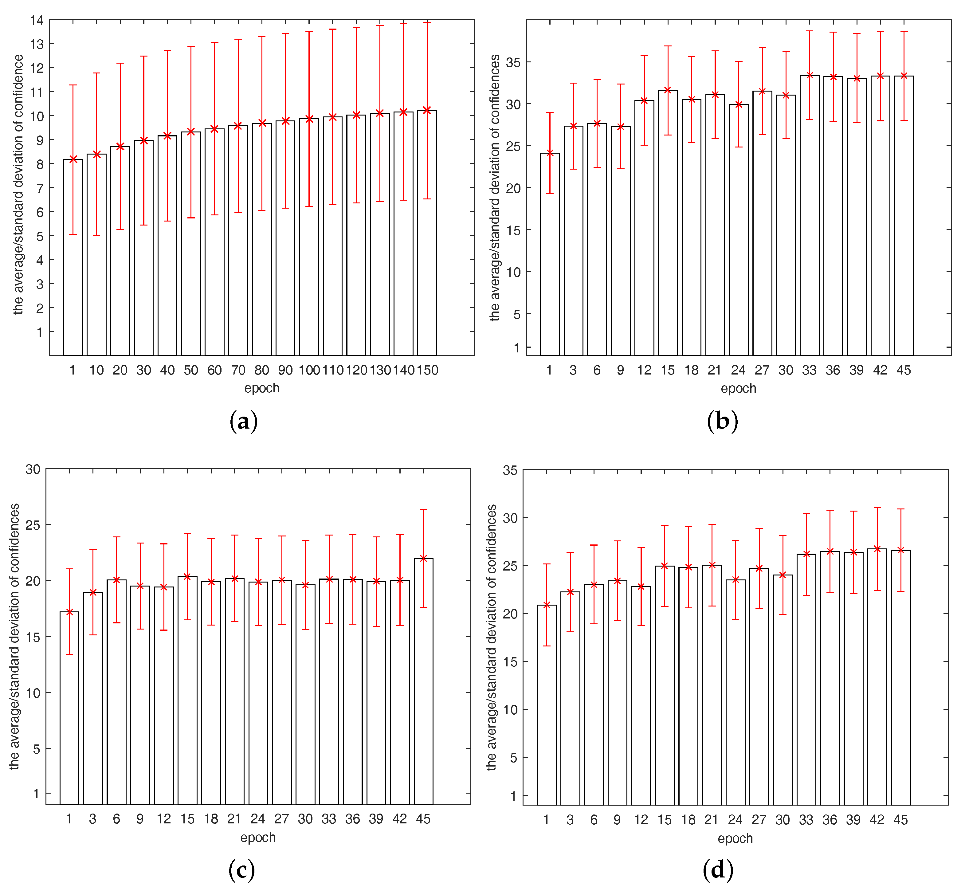
The number of retained connections is dynamic self-adaptive along with the training process. Figure 1 explains the intentions of the self-adaptive sampling probability. The average confidence of all connections tends to be higher and higher with the training process, while the network carries more variations by training. Intuitively, the quality of the connections should be better and better from the random initialization of weights to the well-trained weights. Thus, the self-adaptive sampling probability is in view. Min-Max normalization of confidence is carried out, and then the sampling probability is calculated as follows:
where and are the dropping ratio at the th iteration and -th the iteration, respectively, while and are the ratio for retaining connections. and is a constant between 0 and 1. The initial value could be set as the dropping ratio of ConfNet at the first iteration, or 0.5, for simplicity’s sake.
4.5. Training with Back-Propagation
In Algorithm 1, a regularization mask M for weights W is calculated. A reduced NN is obtained by while b remain unchanged. Then, the reduced NN would be trained by back-propagation. The training of ConfNet or Stochastic ConfNet stops when the classification error converges on the training dataset. The above approach is described in Algorithm 2.
| Algorithm 2: Training with Back-propagation. | |
| Input: A fully connected layer of a DNN with input ; N input samples | |
| Output: weights W and biases b | |
| 1 | Initialize W and b |
| 2 | while classification error converges do |
| 3 | Calculate the mask M via Algorithm 1 |
| 4 | Reduce NN by |
| 5 | Feed-forward: |
| 6 | Differentiate loss with respect to W and b |
| 7 | Update W and b using the back-propagated gradients |
| 8 | end |
| 9 | returnW and b |
5. Experiments
5.1. Experimental Setup
The MNIST dataset [28] consists of pixel handwritten digit images. The task is to classify the images into 10 digit classes. Each digit has the 60,000 training images and 10,000 test images. We scale the pixel values to the range before inputting to our models. The model includes an 800-unit fully connected layer, denoted as ➀, and the sigmoid activation function is adopted, with pre-training [15]. We also test a model with two 800-unit fully connected layers, denoted as ➁, and sigmoid activation function is adopted, without pre-training. Back-propagation is used to train neural networks with the learning rate setting at 0.1. No data augmentation is utilized in the experiments.
The CIFAR-10 dataset [29] consists of natural RGB images. The task is to classify the images into 10 classes. Each class has 50,000 training images and 10,000 testing images. We also scale the pixel values to the and subtract the mean value of each channel computed over the dataset for each image. The feature extractor is: a convolutional layer with 32 feature maps and filters, a Max pooling layer with region and stride 2, a convolutional layer with 32 feature maps and filters, a Max pooling layer with region and stride 2, a convolutional layer with 64 feature maps and filters, and a Max pooling layer with region and stride 2. After that, we input the extracted features into a fully connected layer with 64 units. Sigmoid activation functions is used. Regularization is applied on the fully connected layer. No pre-training is used.
The CIFAR-100 dataset [29] is similar to the CIFAR-10, while the task is to classify images into 100 classes. Each class has 600 images, including 500 training images and 100 testing images. The feature extractor, parameter and training setting are the same as CIFAR-10 except that there are two fully connected layers with 128 units, respectively, on the top of the feature extractor. Sigmoid activation functions are used. Regularization is applied on both of the two fully connected layers. No pre-training is used.
5.2. Experimental Results
The classification results on MNIST, CIFAR-10 and CIFAR-100 are shown in Table 1. On all experimental datasets, the DNNs with regularization achieve better performances than the DNNs without regularization. This could reflect the existence of overfitting during training, and the effectiveness of regularization method (reducing DNN). Moreover, in most cases, the test classification errors of the DNNs with data-dependent regularization (i.e., Confnet, Stochastic ConfNet) are obviously lower than the DNNs with data-independent regularization (i.e., Dropout, DropConnect). Among all experimental datasets, the Stochastic ConfNet gives the best performances, whether for the top-1 classification errors or for the top-5 classification errors. The Confnet also performs well.
The next experimental analyses are all based on the experimental phenomena on MNIST. Figure 2a displays the train error curve and test error curve along with the training iteration. We can see that the gap between train error curve and test error curve is reduced by regularization, and all DNNs with regularization (Dropout, DropConnect, ConfNet and Stochastic ConfNet) significantly outperform the fully connected DNNs. The ConfNet and Stochastic ConfNet achieve superior performance.
Figure 2b shows the performance of different regularization methods with the increase of network size. Seven setups for the number of hidden units, i.e., , are tested. For almost all model sizes, ConfNet and Stochastic ConfNet consistently give a lower error rate than the fully connected DNNs, especially for larger model sizes (e.g., 800, 1000).
In Figure 3a, the average confidence of each model increases steadily over epochs, especially ConfNet and Stochastic ConfNet. It is reasonable that the network would carry more useful information with training, and the regularization by ConfNet and Stochastic ConfNet achieve it better. Figure 3b is about the standard deviation of confidence of the connections. The large standard deviation means a strong ability of discovering the significant connections. Stochastic ConfNet is most outstanding on these two indices.
In Figure 4, the confidence of connections is processed by normalization.The x-axis means confidence with normalization, and distribution of confidence on several different epochs are shown in Figure 4. With the increase of training iterations, the distribution curve of confidence moves to the right continually. It means that the confidence becomes larger with training, while the network carries more useful information.
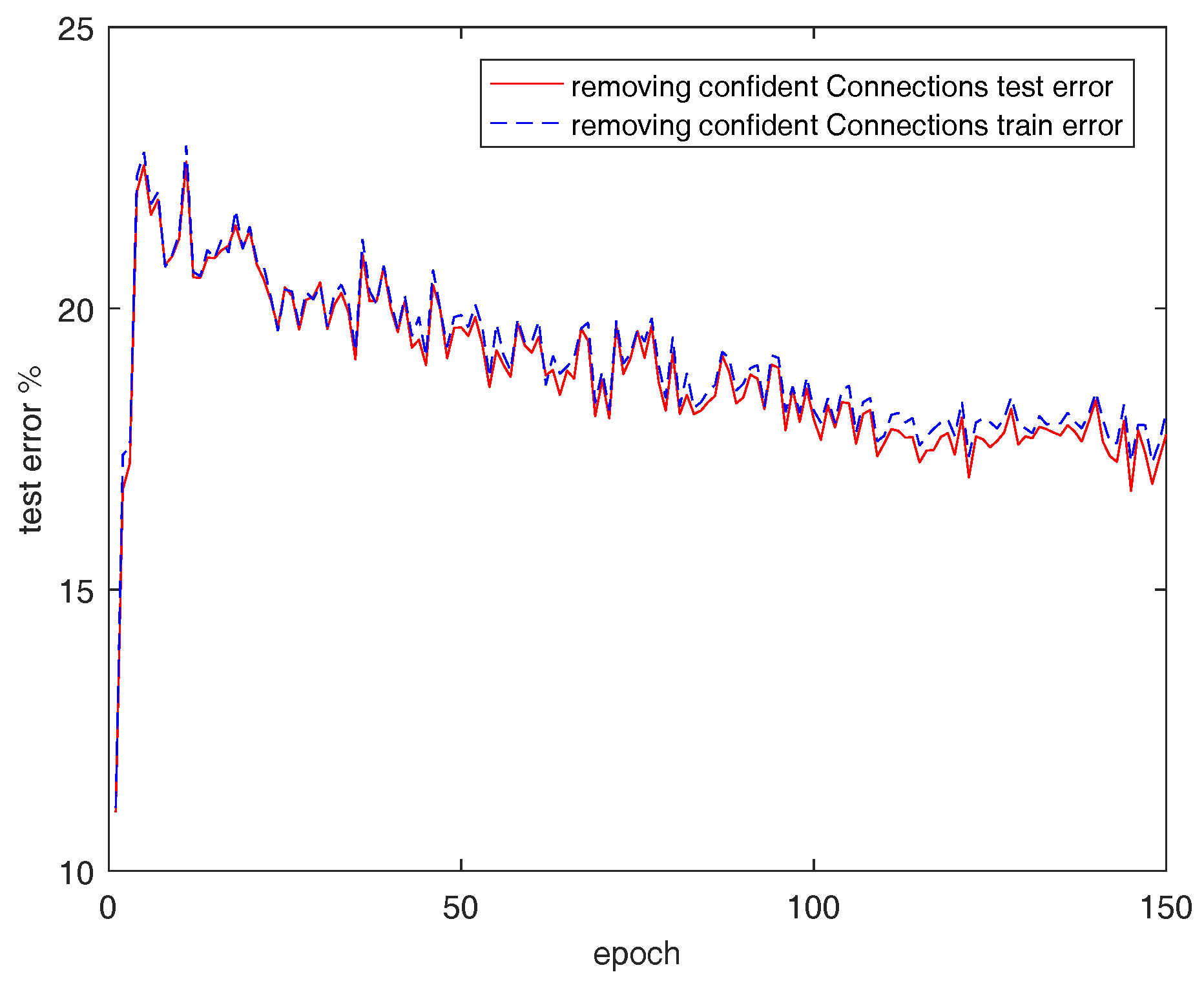
A checking experiment that removes confident connections at each epoch is also implemented. Figure 5 shows the results. The test error remains high, and model can not be convergent. At about 150 epochs, the test error fluctuates at around test errors.
6. Conclusions
In conventional regularization methods (Dropout, DropConnect), the network is regularized by randomly drawing a sub-network from a uniform prior. In this paper, we propose a data-dependent regularization method inspired by the Confident Information First (CIF) principle based on Information Geometry. We have proven that retaining highly confident connections means that the more primary likelihood-structure is preserved, and such a strategy is consistent with the AIC. Moreover, a self-adaptive probabilistic sampling process is used to fit the change of confidence along training to obtain more effective regularization. Empirical evaluation results have demonstrated the superiority of our approach.
Our future research will be focused on the following directions. First, a more generalized theory to demonstrate the relationships among CIF, compressed sensing and random projection will be explored. Second, the ConfNet is currently obtained by a greedy algorithm, so the relative error and time complexity need to be measured. Third, there is a sampling process before calculating the confidence of a connection, which has a negative impact on efficiency. Therefore, a more efficient method will be investigated. Fourth, the application and evaluation of the proposed methods on extra large networks and extending them onto the convolution layer will also be considered in future work.
Acknowledgments
This work is funded in part by the Chinese 863 Program (grant No. 2015AA015403), the Key Project of Tianjin Natural Science Foundation (grant No. 15JCZDJC31100), the Tianjin Younger Natural Science Foundation (Grant No. 14JCQNJC00400), the Major Project of Chinese National Social Science Fund (grant No. 14ZDB153) and MSCA-ITN-ETN - European Training Networks Project (grant No. 721321, QUARTZ).
Author Contributions
Theoretical study and proof: Shengnan Zhang and Yuexian Hou. Conceived and designed the experiments: Shengnan Zhang, Benyou Wang. Performed the experiments: Shengnan Zhang. Analyzed the data: Shengnan Zhang, Benyou Wan. Wrote the manuscript: Shengnan Zhang, Dawei Song, Benyou Wang and Yuexian Hou. All authors have read and approved the final manuscript.
Conflicts of Interest
The authors declare no conflict of interest.
References
- Hinton, G.; Deng, L.; Yu, D.; Dahl, G.E.; Mohamed, A.; Jaitly, N.; Senior, A.; Vanhoucke, V.; Nguyen, P.; Sainath, T.N. Deep Neural Networks for Acoustic Modeling in Speech Recognition. IEEE Signal Process. Mag. 2012, 29, 82–97. [Google Scholar] [CrossRef]
- Mikolov, T.; Deoras, A.; Povey, D.; Burget, L. Strategies for training large scale neural network language models. In Proceedings of the 2011 IEEE Workshop on Automatic Speech Recognition and Understanding (ASRU), Waikoloa, HI, USA, 11–15 December 2011; pp. 196–201. [Google Scholar]
- Sainath, T.N.; Mohamed, A.R.; Kingsbury, B.; Ramabhadran, B. Deep convolutional neural networks for LVCSR. In Proceedings of the 2013 IEEE International Conference on Acoustics, Speech and Signal Processing (ICASSP), Vancouver, BC, Canada, 26–31 May 2013; pp. 8614–8618. [Google Scholar]
- Krizhevsky, A.; Sutskever, I.; Hinton, G.E. ImageNet Classification with Deep Convolutional Neural Networks. Adv. Neural Inf. Process. Syst. 2012, 25, 2012. [Google Scholar] [CrossRef]
- Farabet, C.; Couprie, C.; Najman, L.; Lecun, Y. Learning Hierarchical Features for Scene Labeling. IEEE Trans. Pattern Anal. Mach. Intell. 2013, 35, 1915–1929. [Google Scholar] [CrossRef] [PubMed]
- Tompson, J.; Jain, A.; Lecun, Y.; Bregler, C. Joint Training of a Convolutional Network and a Graphical Model for Human Pose Estimation. In Proceedings of the 27th International Conference on Neural Information Processing Systems, Montreal, QC, Canada, 8–13 December 2014; pp. 1799–1807. [Google Scholar]
- Collobert, R.; Weston, J. A unified architecture for natural language processing: Deep neural networks with multitask learning. In Proceedings of the 25th International Conference on Machine learning, Helsinki, Finland, 5–9 July 2008; pp. 160–167. [Google Scholar]
- Hinton, G.E.; Salakhutdinov, R.R. Reducing the dimensionality of data with neural networks. Science 2006, 313, 504–507. [Google Scholar] [CrossRef] [PubMed]
- Tanner, M.A.; Wong, W.H. The Calculation of Posterior Distributions by Data Augmentation. J. Am. Stat. Assoc. 1987, 82, 528–540. [Google Scholar] [CrossRef]
- Srivastava, N.; Hinton, G.; Krizhevsky, A.; Sutskever, I.; Salakhutdinov, R. Dropout: A simple way to prevent neural networks from overfitting. J. Mach. Learn. Res. 2014, 15, 1929–1958. [Google Scholar]
- Wan, L.; Zeiler, M.; Zhang, S.; Cun, Y.L.; Fergus, R. Regularization of neural networks using dropconnect. In Proceedings of the 30th International Conference on International Conference on Machine Learning, Atlanta, GA, USA, 16–21 June 2013; pp. 1058–1066. [Google Scholar]
- Specht, D.F. Probabilistic Neural Networks. Neural Netw. 1990, 3, 109–118. [Google Scholar] [CrossRef]
- Zhao, X.; Hou, Y.; Song, D.; Li, W. A Confident Information First Principle for Parameter Reduction and Model Selection of Boltzmann Machines. IEEE Trans. Neural Netw. Learn. Syst. 2017. [Google Scholar] [CrossRef] [PubMed]
- Amari, S.; Kurata, K.; Nagaoka, H. Information geometry of Boltzmann machines. IEEE Trans. Neural Netw. 1992, 3, 260–271. [Google Scholar] [CrossRef] [PubMed]
- Hinton, G.E.; Osindero, S.; Teh, Y.W. A fast learning algorithm for deep belief nets. Neural Comput. 2006, 18, 1527–1554. [Google Scholar] [CrossRef] [PubMed]
- Hou, Y.; Zhao, X.; Song, D.; Li, W. Mining pure high-order word associations via information geometry for information retrieval. ACM Trans. Inf. Syst. 2013, 31, 293–314. [Google Scholar] [CrossRef]
- Amari, S.; Nagaoka, H. Methods of Information Geometry (Translations of Mathematical Monographs); American Mathematical Society: Providence, RI, USA, 2007. [Google Scholar]
- Rao, C.R. Information and the Accuracy Attainable in the Estimation of Statistical Parameters; Springer: New York, NY, USA, 1945; pp. 235–247. [Google Scholar]
- Kass, R.E. The Geometry of Asymptotic Inference. Stat. Sci. 1989, 4, 188–219. [Google Scholar] [CrossRef]
- Zhao, X.; Hou, Y.; Song, D.; Li, W. Extending the extreme physical information to universal cognitive models via a confident information first principle. Entropy 2014, 16, 3670–3688. [Google Scholar] [CrossRef]
- Gibilisco, P.; Riccomagno, E.; Rogantin, M.P.; Wynn, H.P. Algebraic and Geometric Methods in Statistics; Cambridge University Press: Cambridge, UK, 2010. [Google Scholar]
- Cencov, N.N. Statistical Decision Rules and Optimal Inference; American Mathematical Society: Providence, RI, USA, 1982. [Google Scholar]
- Hinton, G.E.; Srivastava, N.; Krizhevsky, A.; Sutskever, I.; Salakhutdinov, R.R. Improving neural networks by preventing co-adaptation of feature detectors. arXiv, 2012; arXiv:1207.0580. [Google Scholar]
- Amari, S.I. Information geometry on hierarchy of probability distributions. IEEE Trans. Inf. Theory 2001, 47, 1701–1711. [Google Scholar] [CrossRef]
- Akaike, H. IEEE Xplore Abstract—A new look at the statistical model identification. IEEE Trans. Autom. Control 1974, 19, 716–723. [Google Scholar] [CrossRef]
- Bozdogan, H. Model selection and Akaike’s Information Criterion (AIC): The general theory and its analytical extensions. Psychometrika 1987, 52, 345–370. [Google Scholar] [CrossRef]
- Nakahara, H.; Amari, S.I. Information-geometric measure for neural spikes. Neural Comput. 2002, 14, 2269–2316. [Google Scholar] [CrossRef]
- Lecun, Y.; Bottou, L.; Bengio, Y.; Haffner, P. Gradient-based learning applied to document recognition. Proc. IEEE 1998, 86, 2278–2324. [Google Scholar] [CrossRef]
- Krizhevsky, A.; Hinton, G. Learning Multiple Layers of Features from Tiny Images. Available online: http://www.cs.utoronto.ca/kriz/learning-features-2009-TR.pdf (accessed on 26 June 2017).
Figure 1.
The average and standard deviation of confidence of connections. (a) the connections of the fully connected layer on MNIST; (b) the connections of the first fully connected layer on CIFAR10; (c) the connections of the first fully connected layer on CIFAR100; (d) the connections of the second fully connected layer on CIFAR100.

Figure 2.
The classification performances on MNIST. (a) the classification performances on MNIST as the iterations progress; (b) the classification performances on MNIST for different model sizes.
Figure 2.
The classification performances on MNIST. (a) the classification performances on MNIST as the iterations progress; (b) the classification performances on MNIST for different model sizes.

Figure 3.
The average and standard deviation of confidence of the connections in the training phase on MNIST. (a) the average confidence of the connections; (b) the standard deviation of confidence of the connections.
Figure 3.
The average and standard deviation of confidence of the connections in the training phase on MNIST. (a) the average confidence of the connections; (b) the standard deviation of confidence of the connections.
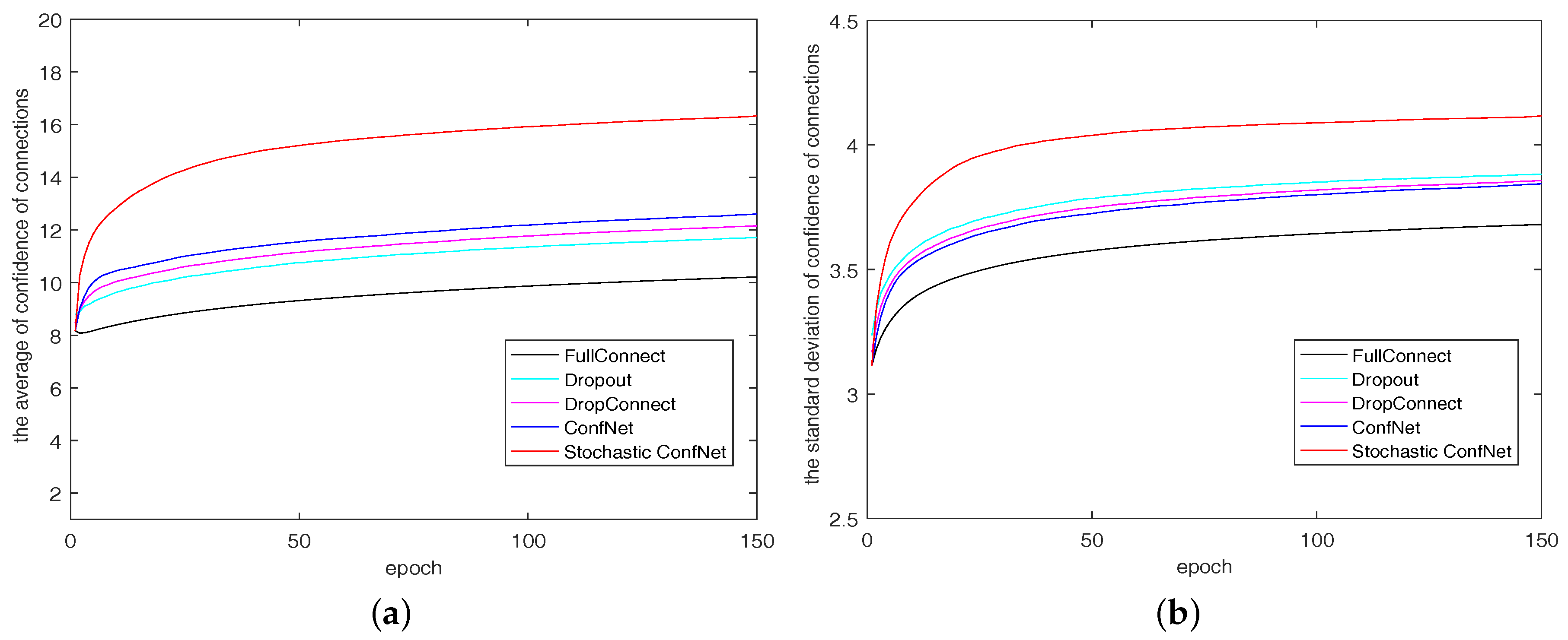
Figure 4.
The distribution of confidence of connections in the training phase on MNIST. (a) the distribution of confidence of connections in the training phase; (b) the magnified Figure 4a.
Figure 4.
The distribution of confidence of connections in the training phase on MNIST. (a) the distribution of confidence of connections in the training phase; (b) the magnified Figure 4a.
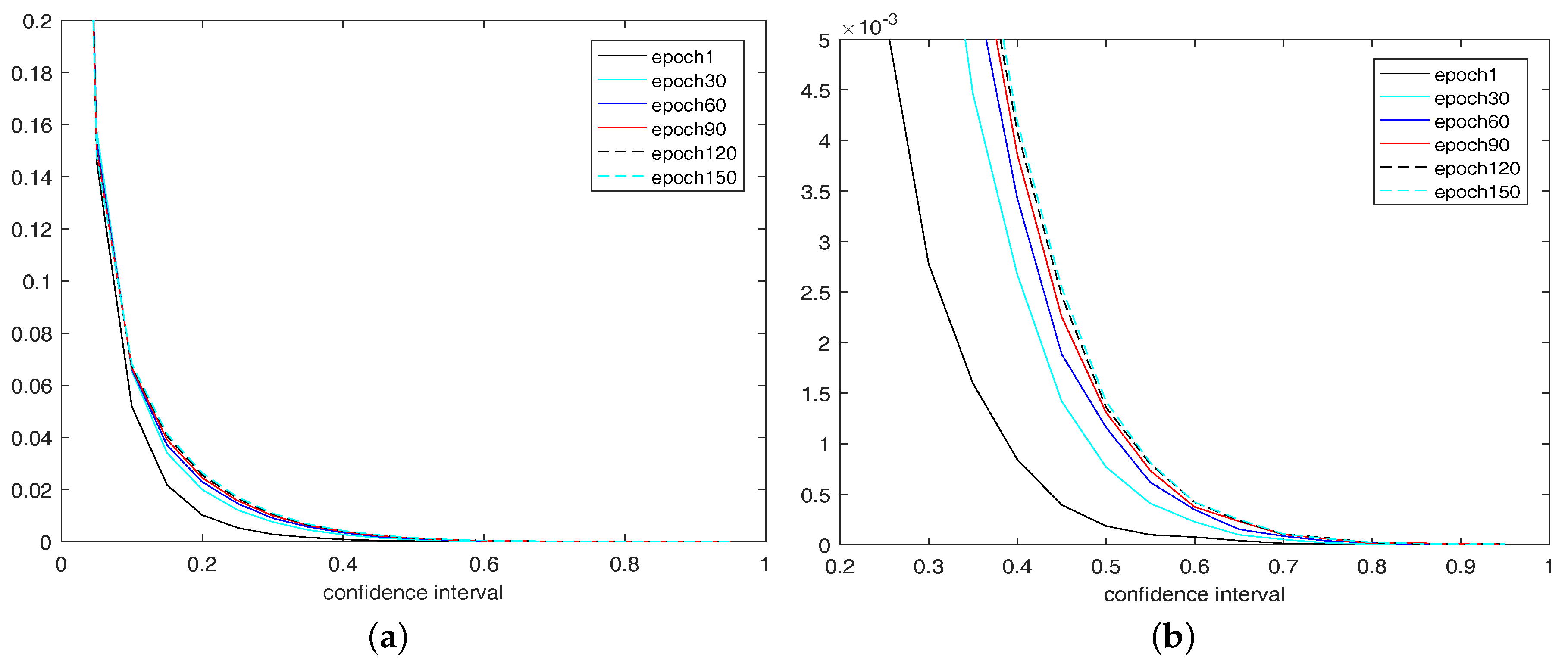
Figure 5.
The classification performances on MNIST with the removal of confident connections.


Table 1.
Comparison of test classification errors (%).
| Model | MNIST | CIFAR-10 | CIFAR-100 | |||
|---|---|---|---|---|---|---|
| Top-1 ➀ | Top-1 ➁ | Top-1 | Top-5 | Top-1 | Top-5 | |
| FullConnect | 1.84 | 1.56 | 20.09 | 1.32 | 52.02 | 23.26 |
| Dropout | 1.79 | 1.43 | 19.87 | 1.24 | 51.18 | 23.02 |
| DropConnect | 1.77 | 1.59 | 18.53 | 1.19 | 50.87 | 22.79 |
| Confnet | 1.62 | 1.19 | 19.48 | 1.31 | 50.06 | 22.74 |
| Stochastic ConfNet | 1.50 | 1.19 | 18.25 | 1.12 | 48.39 | 19.96 |
The results in bold are the results with lowest error rate. On MNIST, the retained probability p of Dropout is ; the retained probability p of DropConnect is ; the hyper-parameters and of Stochastic ConfNet are and , respectively; and the initial value is . On CIFAR-10, the retained probability p of Dropout is ; the retained probability p of DropConnect is ; the hyper-parameters and of Stochastic ConfNet are and , respectively; and the initial value is . On CIFAR-100, the retained probability p of Dropout is ; the retained probability p of DropConnect is ; the hyper-parameters and of Stochastic ConfNet are and , respectively; and the initial value is .
© 2017 by the authors. Licensee MDPI, Basel, Switzerland. This article is an open access article distributed under the terms and conditions of the Creative Commons Attribution (CC BY) license (http://creativecommons.org/licenses/by/4.0/).
Share and Cite
MDPI and ACS Style
Zhang, S.; Hou, Y.; Wang, B.; Song, D. Regularizing Neural Networks via Retaining Confident Connections. Entropy 2017, 19, 313. https://doi.org/10.3390/e19070313
AMA Style
Zhang S, Hou Y, Wang B, Song D. Regularizing Neural Networks via Retaining Confident Connections. Entropy. 2017; 19(7):313. https://doi.org/10.3390/e19070313
Chicago/Turabian StyleZhang, Shengnan, Yuexian Hou, Benyou Wang, and Dawei Song. 2017. "Regularizing Neural Networks via Retaining Confident Connections" Entropy 19, no. 7: 313. https://doi.org/10.3390/e19070313
Note that from the first issue of 2016, this journal uses article numbers instead of page numbers. See further details here.