Entropy Characterization of Random Network Models


1
Departamento Matemática Aplicada a las TIC, ETSI Telecomunicación, Universidad Politécnica de Madrid, E-28040 Madrid, Spain
2
Information Processing and Telecommunications Center (IPTC), Universidad Politécnica de Madrid, E-28040 Madrid, Spain
*
Author to whom correspondence should be addressed.
Entropy 2017, 19(7), 321; https://doi.org/10.3390/e19070321
Submission received: 31 May 2017
/
Revised: 24 June 2017
/
Accepted: 27 June 2017
/
Published: 30 June 2017
(This article belongs to the Special Issue Complex Systems, Non-Equilibrium Dynamics and Self-Organisation)
Abstract
:This paper elaborates on the Random Network Model (RNM) as a mathematical framework for modelling and analyzing the generation of complex networks. Such framework allows the analysis of the relationship between several network characterizing features (link density, clustering coefficient, degree distribution, connectivity, etc.) and entropy-based complexity measures, providing new insight on the generation and characterization of random networks. Some theoretical and computational results illustrate the utility of the proposed framework.
1. Introduction
The modelling of complex systems via networks or graphs [1,2,3] has become a well established research field due to the fact that many different complex systems share some essential common features that can be gathered in a Network Model (NM) [4]. Although network elements can represent very different entities depending on the system being analyzed, still some common characteristics seem to be ubiquitous in many models. For instance, common patterns usually appear in social networks [5], biology networks [6], technological networks [7,8] or information networks [9,10].
Most of the common features of these (usually very large) networks rely on statistical properties; hence, some types of NMs have been successfully employed for characterizing such networks. Starting from the seminal model [11] which served as a baseline for comparative purposes, several more sophisticated models have been proposed to explain the behavior of complex networks [3,9,12,13].
The characterization of complex networks can be addressed by considering each network either as an isolated and unique entity or as a sample (i.e., an outcome) from a random experiment. The latter perspective is grounded on constructing a probability space (i.e., a probability measure on the space of possible networks); this probability model allows for a compact network characterization and it can be employed for several purposes (e.g., link detection or prediction). In this paper, we formalize this perspective to rigorously define Random Network Models (RNMs) and characterize their properties. The relationship between some network features such as link density, clustering coefficient, degree distribution and connectivity, is analyzed from the point of view of the RNM complexity measured in terms of some defined entropies.
The paper is organized as follows: Section 2 formalizes the concept of RNM and illustrates some existing network models from this formal perspective. The role of different network properties and their characterization via model-derived random variables is considered in Section 3, with the aim of assessing the role of restrictive network features in the complexity of the corresponding RNMs. In Section 4, the entropy of the RNMs is considered and some theoretical results are presented to illustrate its role in characterizing model complexity. Section 5 addresses the entropies associated with derived random variables (mainly, degree distributions), as alternative measures of complexity and explores their relationship with model entropy. Section 6 presents computational results that illustrate the relationship between the considered network features and complexity. The paper finishes with some concluding remarks in Section 7.
2. Probability Models for Network Generation: Random Network Models
The simplest random network generation models define a probability space over the the set of all possible networks. Such space can be denoted by , where is the sample space (or set of possible networks), corresponds to the set of all possible events, and P is a probability measure on .
2.1. Sample Space
In order to construct , one has to define the set of elements that characterize any given network. The simplest models are grounded on two sets: V, the set of nodes or vertices, and E, the set of all possible edges or links between elements of V. If , then . In this context, any network is defined by a pair , where . Note that in this case .
2.2. Set of Events
Since is considered to be a finite set, a natural (and the largest) -algebra (set of events) can be defined as . Note that any property defined in relation to networks (e.g., being connected, containing triangles, having a given degree k, etc.) is associated with a given element of the set of events () or a subset of the sample space ().
2.3. Probability Measure
Again, since is finite, it suffices to define , all the elementary events. For a fixed set of nodes V, the random network is defined by a set of random variables (the edge indicators of the network). In general, may be too large for an explicit definition of each ; hence, manageable laws are desirable for defining P, based on simplifying or regularity assumptions.
Typically, a hypothesis such as distribution uniformity or independence among some variables (considered to represent known properties of the phenomenon to be modelled) are employed, allowing for an easier construction or definition of P. In the following, we illustrate different simplifying procedures for constructing different P measures or distributions.
Following the standard notation in random variables, when considering an RNM, we will denote by G the general outcome of the random experiment, whereas we will denote by a specific sample network outcome. It is important to note that a given sample , obtained as the sample outcome from a specific RNM, could have been obtained as the sample outcome from a different model (having a different P measure or distribution). Hence, typical expressions such as “being a type 1 network” should be qualified to “ being a network generated from a type 1 model”.
In the following subsections, we illustrate some known network models from the RNM perspective.
2.3.1. Erdös–Renyi (ER) Model [14]
This network generating procedure is grounded on a uniformity assumption. It considers as the set of networks with n vertices, and it defines:
where is the set of networks having m edges, whose size is given by , where .
Networks created following the ER procedure (i.e., following the ER model) are usually called ER networks. We claim that they should be labeled as networks obtained from the ER model.
2.3.2. Gilbert Model [15]
This RNM considers that each of the edge indicators is a Bernoulli random variable with probability p (with same value of p for each link). The number of edges in the networks generated by this model follows a Binomial distribution with parameters and p. Hence, the probability of a network , having set of edges , is:
Note that the distribution of , conditioned to having a fixed number of edges (i.e., ), becomes:
thus being equivalent in such case to the ER model. Both Gilbert and ER models tend to be confused frequently in the existing literature.
2.3.3. Random Networks with Hidden Variables
In these models, the probabilities associated with the establishment of links between pairs of nodes depend on some hidden variables [16,17]. As a special case, Range or Distance Dependent Random Graphs [18,19] consider that each edge indicator is a Bernoulli random variable with probability , where is the range (i.e., a measure that can represent, for instance, a physical or a social distance) between the pair of nodes linked by . These RNMs generalize the previous Gilbert model.
2.3.4. Kronecker Graphs [20]
These models are based on the generation of matrices via Kronecker products, being mathematically tractable while generating networks with desired structural properties (heavy tail distribution, densification, etc.).
2.3.5. Exponential Random Graphs Models (ERGMs) [21]
Random Networks can be generally modelled by:
where is a vector of parameters and s is a vector of features (sufficient statistics). In general, for any type of random network distribution, the size of s could be huge, each component gathering information associated with any arbitrary subset of nodes in the network.
ERGM models are grounded on some simplifying assumptions that allow for an easy definition or characterization of P via conditional probabilities. This fact guarantees that the definition of the distribution only requires a reduced set of features, which allows for a good practical applicability.
ERGMs can be seen as a type of Markov Graph [22], which defines a sub-family of distributions (or measures) for graphs with even stronger simplifying conditional independence properties. A random graph is a Markov Graph if non-incident edges (i.e., edges between disjoint pairs of nodes) are independent conditional on the rest of the graph. The Markov Graph assumption guarantees that the the set of features only needs to consider triangles and k-stars. (Note that the term Markov Network or Markov Field is also employed when considering dependence graphs for random variables; here, we use the term to refer to families of distributions on networks.).
2.4. Inference of Random Network Models
If we consider a given network to be a sample from an RNM, strong assumptions (i.e., inductive bias) must be imposed for carrying out a model inference from that single sample network (a similar circumstance shows up when addressing parameter estimation for vector joint distributions by making use of a single or few vector samples). Such estimation procedures can be carried out if strong simplifying assumptions are assumed in the model: e.g., some components (in our case, sub-networks) may be considered as having the same distribution, or some Markov type properties may be assumed in the joint distributions.
Inference of Markov Graphs
The Markov Graph model assumption provides a strong inductive bias which also allows for model inference from a single sample (network). Usually, the inference procedure to obtain P is carried out as follows: the ERGM structure is assumed on P and, given a (sample) network and a set s of chosen features (number of links, number of triangles, etc.), a maximum likelihood estimate for is constructed. The resulting network distribution model maximizes the likelihood of the sample network and all networks with the same features s [23]. This fundamental procedure can be applied to a whole family of models [24]. Nevertheless, the standard likelihood techniques for the Markov models are not immediately applicable because of the complicated functional dependence of the normalizing constant on the parameters. Hence, practical estimation procedures need to perform a sampling in the network (which could also be interpreted as analyzing an appropriate sub-network) via, for instance, Gibbs sampling [25], pseudo-likelihood techniques [26], or stochastic approximation based procedures [27,28].
In the following sections, we will try to characterize some network features and their relationship with the RNM, with the aim of helping to estimate the nature and complexity of such model.
3. Network Properties and Derived Random Variables: Complexity of Successive Approximation Models
3.1. Network Properties and Derived Random Variables
Given an RNM, different properties can be imposed to the model, many of them being associated with random variables that can be derived from the RNM. For example, any quantifiable property or feature f that can be defined on a sample network (e.g., number of links, number of triangles, node average degree, connectivity as a zero/one variable, etc.) can be characterized via a corresponding random variable F defined as follows:
Definition 1.
Let be the RNM probability space. We define the random variable F as the following P-measurable function:
where is a function that computes a quantifiable property (number of links, number of triangles, sample average degree, connectivity, etc.) in graph g. We denote F as the Random Network Model Feature random variable.
As an example, besides the standard variables corresponding to the number of links (associated with link density) and number of triangles (associated with clustering coefficient), we can also define the Bernoulli variable denoted connectivity that is constructed with f such that if g is disconnected and if g is connected.
A special definition has to be developed when referring to the degree distribution property.
3.1.1. Degree Distribution Associated with an RNM
Given an RNM, we can consider generating a sample network according to such model, and randomly selecting a node of such sample network in order to check its degree. Since such degree random variable is derived from the model, it will be designated as the Random Network Model Degree (RNMD).Formalizing this procedure, the RNMD can be derived from the RNM as follows:
Definition 2.
Let be the RNM probability space, and let be a probability space on the set of nodes V where is the uniform probability measure. Then, let us consider the product measurable space . We define the random variable K as the following measurable function:
where is the degree of node in graph g. We denote K as the Random Network Model Degree (RNMD) random variable, and , the distribution of K, is denoted as the Random Network Model Degree Distribution (RNMDD).
3.1.2. Degree Distribution of a Sample Network
We can finally define an additional random variable that leads to the commonly denoted degree distribution of a network :
Definition 3.
Let be an RNM probability space with corresponding RNMD random variable K(as defined in 2). Let be a sample network from the model. The random variable is the degree variable associated with sample network . The distribution of is the usually denoted degree distribution of network .
Given a sample network , we may want to estimate the degree distribution associated with the model that generated , by computing the “empirical” degree distribution of . In Section 4 and Section 5, the entropies associated with the RNM and some of these distributions will be analyzed as a means of characterizing RNM complexity.
3.2. Successive Approximation Models
If we impose a network to satisfy some specific properties (i.e., some features), the corresponding RNM complexity is affected by such restrictions [29,30,31]. In [29,30], the concept of network ensembles is proposed, based on a statistical mechanics approach, to characterize random networks. These network ensembles can be characterized by their entropy, which, in the simplest case, evaluates the cardinality of networks in the ensemble. In [30], approximate expressions for the cardinality associated with different models (satisfying several restrictions) are provided under some simplifying assumptions (sparse networks with structural cutoff). Alternatively, in [31], the -series methodology is proposed to define a series of null models of random network ensembles.
Hence, given a real network, a sequence of RNMs (or, in the simplest version, networks ensembles) can be considered, where each subsequent model gets more restrictive by imposing an additional structural property or feature (link density, clustering coefficient, degree sequence, etc.) shared with the real network. Such sequence can be interpreted as a means of approximating the model that may best characterize the given network. The evolution of the entropy of these subsequent RNMS quantifies how restrictive the additional constraints become.
A standard first approximation model is usually defined by imposing some density of links in the network. A hard condition may impose, for instance, a fixed number of links, let us say m (e.g., the ER model). This restriction would reduce the total set of possible networks that can be generated (according to the newly restricted model), from the whole set to . On the other hand, a soft condition may assign a probability to each network depending only on its number of links (e.g., the Gilbert model). In this case, the total number of networks that can be generated is not reduced, but their corresponding probability is modified, usually reducing also the complexity of the RNM. This reduction can be measured, for instance, via some complexity measures such as the entropy, as it will be shown in the following Section 4.
Following this reasoning, in a following stage, new restrictions can be imposed to our model, such as the network having a given number of triangles or clustering coefficient. These new restrictions, again, will either reduce the set of possible outcomes or unbalance the probability distribution, hence usually reducing the entropy of the new corresponding model.
Other interesting features considered in this paper are the degree distribution and the connectivity of the network. The degree distribution will show to be a very useful feature since, in general, its entropy is related to the entropy of the RNM. Finally, we will also see that connectivity is strongly dependent on the link density and the clustering coefficient.
4. Entropy of RNMs
In this section, the entropy associated with random network generation models is analyzed. The entropy of random network generation models is computed as the entropy of the generating probability space. Given a probability space as a model underlying the generation of graphs, the entropy [32] of such model is given by:
and it is measured in bit units. For example, if we have no a priori knowledge about the model, we may have to assume that any network can be generated with equal probability , so that the entropy of this uniform model is:
which corresponds to the maximum entropy that we can attain for any P defined in such pair corresponding to networks with n vertices.
The ER model (1) with n nodes and m links has entropy:
whereas the Gilbert model with n nodes and link probability p has entropy [33]:
where and , is the binary entropy function. As mentioned above, the ER and Gilbert models, although being different, are considered as the same model in most of the existing literature when considering . Nevertheless, they are different and they systematically satisfy the following relationship:
Lemma 1.
Proof.
Let us consider the known bound:
If we consider and , taking base-2 logarithms on both sides, we obtain the first inequality. The second inequality is directly obtained from the fact that (note that reaches its maximum value at , when the Gilbert model corresponds to the uniform distribution and ). ☐
Entropy Reduction via Restrictions in the RNM
Some network generation algorithms may follow several steps in the construction procedure. For instance, they may initially create a network with a given number of links (first step), and then, they would apply a rewiring step so that while the number of links is preserved, new network features are imposed (e.g., to increase the number of triangles, and hence the resulting clustering coefficient). In this section, we characterize the entropy reduction caused by the restrictions imposed at each step.
Let us consider an RNM defining a distribution on so that we can partition into sets such that . In such case, we have that
where the last inequality becomes strict whenever there exist such that . Model applies, for instance, when networks with the same number of links are generated with the same probability.
We consider now a new model that preserves each of the ensemble probabilities, while redefining the probability distribution within each , as a result of priorizing new properties of the network. For instance, can model a two-step sample network generation procedure which initially creates a sample from and then modifies it (e.g., via rewiring). In such context, one can prove the following result:
Lemma 2.
Let us consider model such that it defines a distribution satisfying for all . Then:
Proof.
Since , then, based on Jensen’s inequality, we have:
Therefore:
☐
In general, the computation of H must be performed based on analytical knowledge of the generation model. In the case that the network size is small enough, Monte Carlo simulations could be carried out to estimate such entropy.
In the following section, the entropies of derived variables (especially degree distributions) are considered as an alternative way to more easily characterize network complexity.
5. Entropies Associated with Derived Variables and Degree Distributions
The entropy of RNM derived variables can also be employed as an indirect measure of model complexity. For example, the entropy of the number of links variable is zero for the ER model (, since it always generates networks with a prescribed number m of links), whereas the entropy of such a variable for the Gilbert model is given by:
Similarly, the entropy of the Bernoulli variable connectivity can also be computed. In the following, we will focus on the entropies associated with degree distributions.
5.1. Entropies of Degree Distributions
In Section 3, the Random Network Model Degree Distribution (RNMDD) was defined as an alternative feature to the standard (sample) degree distribution corresponding to a specific sample network. Both degree distribution concepts are analyzed here considering some associated entropy measures and how they relate to the entropy of the random network generation model considered in the previous section.
One can define the entropy associated with RNMDD as:
This entropy can be seen as an indicator of the average network heterogeneity from the connectedness point of view, since it measures the diversity of the link distribution.
If we consider the ER network generation model, the associated RNMD variable K follows a hyper-geometric distribution:
which can be approximated, under the corresponding assumptions, by Binomial and Poisson distributions:
On the other hand, if we consider the Gilbert network generation model, the associated RNMD variable K follows a binomial distribution:
Note that provides some information concerning the network generation model. For a given RNM M, and are expected to be related, but there may be cases where a model with high H may have low and vice versa.
When comparing ER and Gilbert models, Lemma 1 defines a bounding relationship between their corresponding model entropies. Comparative computations of and suggest that the entropies of the degree distributions associated with ER and Gilbert models satisfy:
Conjecture 1.
This result can be intuitively justified since, while and are similar in shape, the support of is larger than the support of .
In general, the computation of requires a knowledge of the RNM, which is not always available. As an alternative, we can compute the entropy of the empirical distribution (see Section 3.1.2) as an estimator of . In general, the quality of such estimations will depend on the properties of the model.
5.2. Other Measures of Sample Entropies
For the sake of completeness, other measures of entropies are commented on in this subsection. All of them have been considered in the context of sample networks. These definitions could be extended to the RNM in a similar manner as it has been done above for the standard degree distribution entropy.
In [34,35], the remaining (outward) degree distribution, , of a sample network is proposed. The use of the remaining degree distribution helps for the estimation of degree–degree correlations and hence the network assortativeness. In [35], the (empirical) entropy associated with such remaining degree distribution is analyzed for power law distributions, showing that the increase of the exponent (and the decrease of the cutoff) leads to a reduction of the entropy for the sample network.
In [36], the entropy based on the distribution of the length of cycles is proposed. Such distribution provides information about the existing feedback in the network, and it may indirectly measure the network ability to store information within the network cycles. In general, such distribution seems to be change little with respect to network modifications.
6. Computational Estimations
In this section, link density, clustering coefficient, degree distributions and connectivity are computed and comparatively analyzed in order to illustrate their relationship with RNM complexity. The fundamental simulations have been performed by imposing varying values of the link density and triangle density parameters in ERGMs.
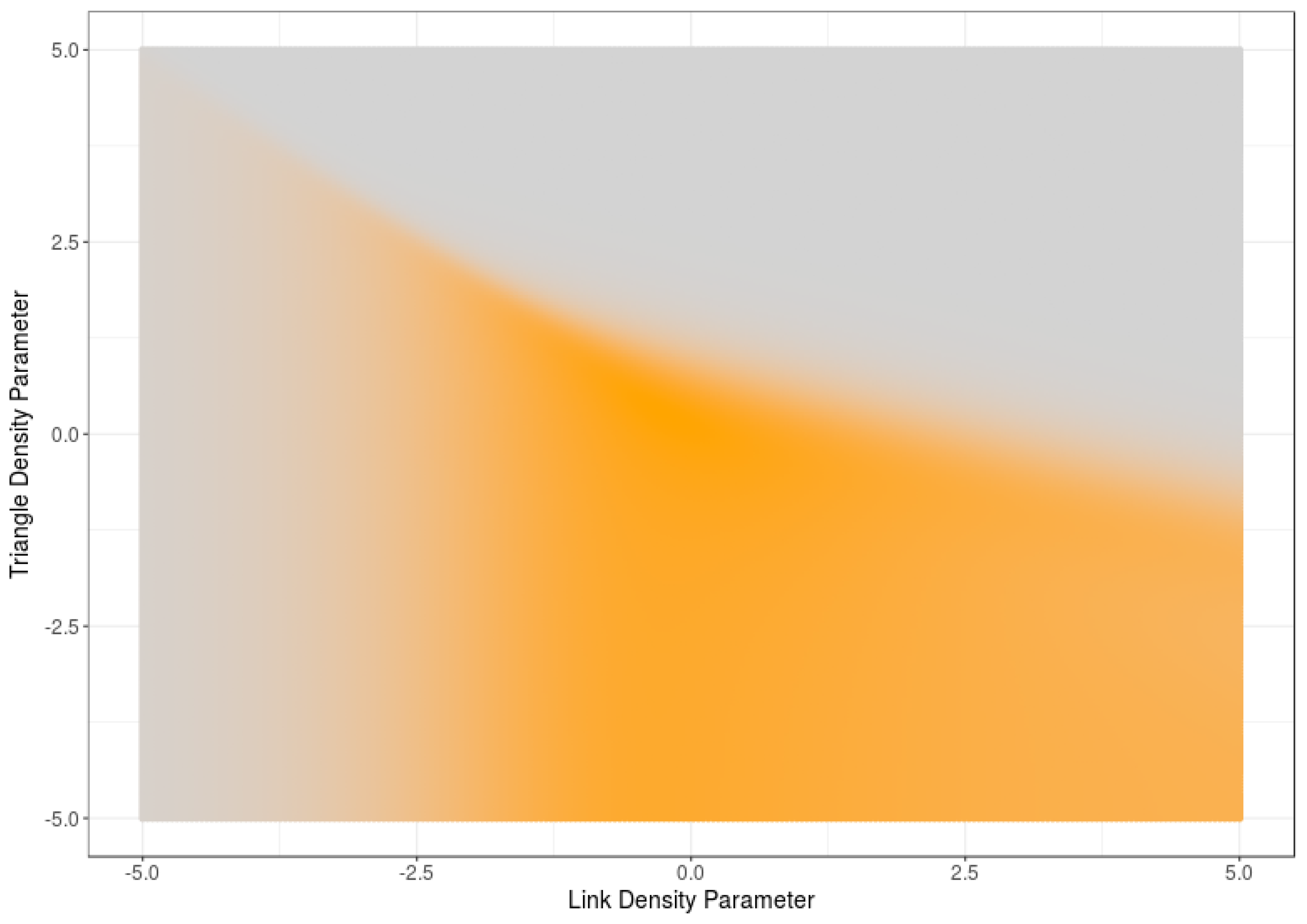
Figure 1 displays the entropy of 5-node RNMs as a function of the link and triangle density parameters. High values of entropy correspond with orange colors. Note that the maximum entropy is mainly reached for a medium number of edges and triangles. If too few or too many links are imposed, the RNM entropy is reduced. Such maximum does not change significantly if the required number of triangles is reduced, but it drops drastically if a larger number of triangles is imposed.
Figure 2 displays the average sample degree entropy of 5-node RNMs as a function of the link and triangle density parameters. Note that the results are quite similar to the ones obtained in Figure 1. This result suggests that high (low) values of sample degree entropy correspond with high (low) values of model entropy.
Figure 3 displays, for a set of 5-node RNMs generated with varying triangle densities, the relationship between the model entropy and its average sample degree entropy. The orange color indicates the level of the triangle density parameter associated with each model. Note that, for large triangle densities, both entropies tend to follow a linear relationship, which may be distorted only for some networks with a reduced triangle density. These results support the above claimed correlation between sample degree entropy and model entropy.
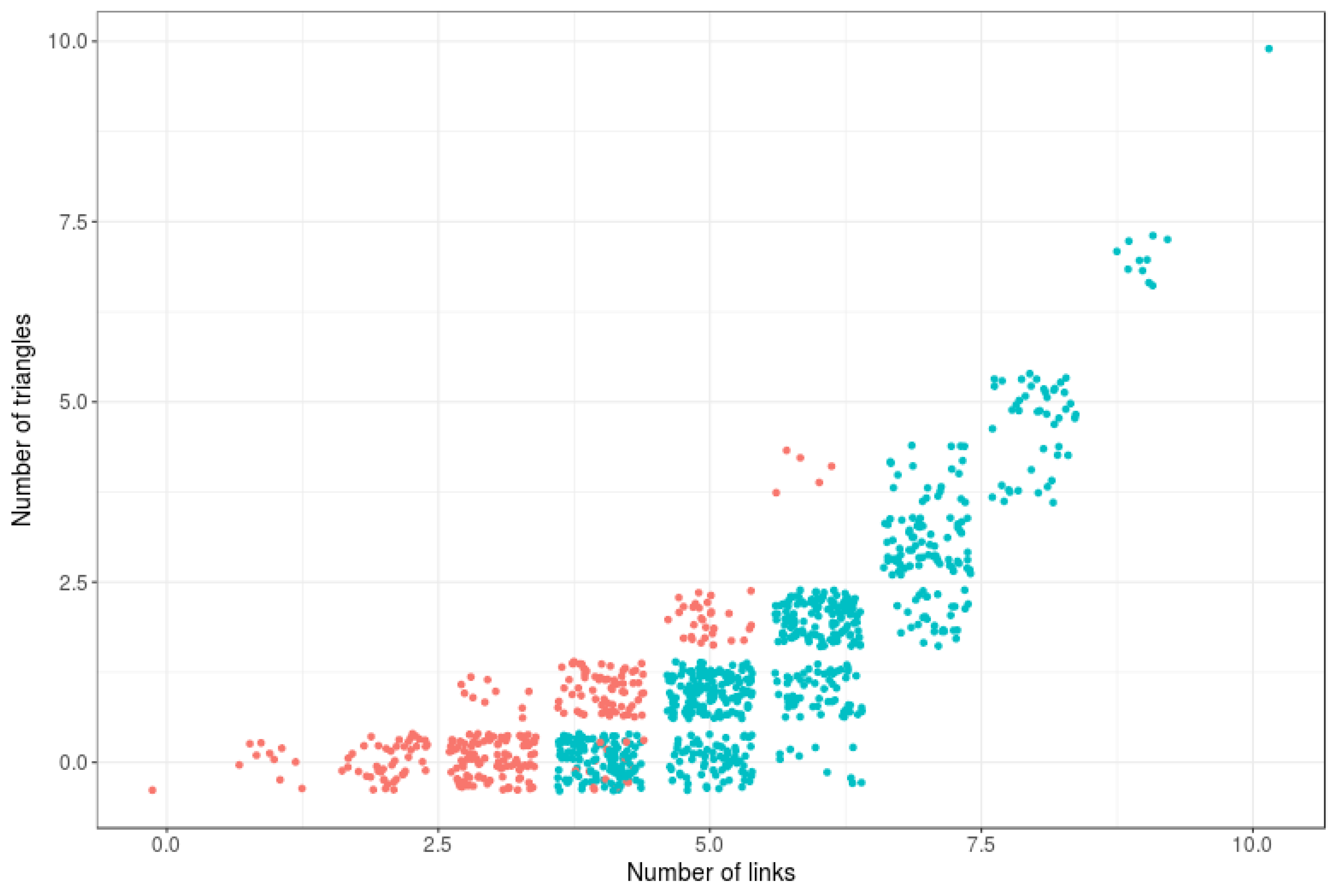
Figure 4 illustrates, for a set of 6-node RNMs, the strong relationship between link density, triangle density and network connectivity. Hence, if these features are jointly imposed in an arbitrary manner (against their natural relationship) on an RNM, the entropy of such model may drop drastically.
7. Conclusions
A mathematical framework has been proposed for analyzing Random Network Models (RNMs) and for characterizing their complexity. Such framework allows the study of several network properties or features (link density, clustering coefficient, degree distribution, connectivity), and their relationship with the RNM complexity. For doing so, different entropy measures have been evaluated and their relationship has been assessed. The sample degree distribution entropy has shown to be correlated with the RNM entropy, providing a practical measurable indicator of complexity in real networks.
Acknowledgments
This work has been partially supported by project MTM2015-67396-P of Ministerio de Economía y Competitividad, Spain.
Author Contributions
Pedro J. Zufiria developed the theoretical content, wrote the document and helped with the simulations. Iker Barriales-Valbuena developed the simulations and helped with the theoretical content and the writing of the paper. Both authors have read and approved the final manuscript.
Conflicts of Interest
The authors declare no conflict of interest.
References
- Barabási, A.L.; Frangos, J. Linked: The New Science of Networks Science of Networks; Basic Books: New York, NY, USA, 2014. [Google Scholar]
- Newman, M.E. The structure and function of complex networks. SIAM Rev. 2003, 45, 167–256. [Google Scholar] [CrossRef]
- Watts, D.J.; Strogatz, S.H. Collective dynamics of “small-world” networks. Nature 1998, 393, 440–442. [Google Scholar] [CrossRef] [PubMed]
- Dorogovtsev, S.N.; Mendes, J.F. Evolution of Networks: From Biological Nets to the Internet and WWW; Oxford University Press: Oxford, UK, 2013. [Google Scholar]
- Onnela, J.P.; Saramäki, J.; Hyvönen, J.; Szabó, G.; Lazer, D.; Kaski, K.; Kertész, J.; Barabási, A.L. Structure and tie strengths in mobile communication networks. Proc. Natl. Acad. Sci. USA 2007, 104, 7332–7336. [Google Scholar] [CrossRef] [PubMed]
- Jeong, H.; Tombor, B.; Albert, R.; Oltvai, Z.N.; Barabási, A.L. The large-scale organization of metabolic networks. Nature 2000, 407, 651–654. [Google Scholar] [PubMed]
- Faloutsos, M.; Faloutsos, P.; Faloutsos, C. On Power-Law Relationships of the Internet Topology; ACM: New York, NY, USA, 1999; pp. 251–262. [Google Scholar]
- Chen, Q.; Chang, H.; Govindan, R.; Jamin, S. The origin of power laws in Internet topologies revisited. In Proceedings of the INFOCOM 2002. Twenty-First Annual Joint Conference of the IEEE Computer and Communications Societies, New York, NY, USA, 23–27 June 2002; Volume 2, pp. 608–617. [Google Scholar]
- Barabási, A.L.; Albert, R. Emergence of scaling in random networks. Science 1999, 286, 509–512. [Google Scholar] [PubMed]
- Redner, S. How popular is your paper? An empirical study of the citation distribution. Eur. Phys. J. B Condens. Matter Complex Syst. 1998, 4, 131–134. [Google Scholar] [CrossRef]
- Erdos, P.; Rényi, A. On the evolution of random graphs. Bull. Inst. Int. Stat. 1961, 38, 343–347. [Google Scholar]
- Jackson, M.O.; Rogers, B.W. Meeting strangers and friends of friends: How random are social networks? Am. Econ. Rev. 2007, 93, 890–915. [Google Scholar] [CrossRef]
- Herrera, C.; Zufiria, P.J. Generating scale-free networks with adjustable clustering coefficient via random walks. In Proceedings of the 2011 IEEE Workshop Network Science, West Point, NY, USA, 22–24 June 2011; pp. 167–172. [Google Scholar]
- Erdos, P.; Rényi, A. On random graphs. Publ. Math. Debr. 1959, 6, 290–297. [Google Scholar]
- Gilbert, E.N. Random plane networks. J. Soc. Ind. Appl. Math. 1961, 9, 533–543. [Google Scholar] [CrossRef]
- Caldarelli, G.; Capocci, A.; De Los Rios, P.; Muñoz, M.A. Scale-free networks from varying vertex intrinsic fitness. Phys. Rev. Lett. 2002, 89, 258702. [Google Scholar] [CrossRef] [PubMed]
- Boguñá, M.; Pastor-Satorras, R. Class of correlated random networks with hidden variables. Phys. Rev. E 2003, 68, 036112. [Google Scholar] [CrossRef] [PubMed]
- Grindrod, P. Range-dependent random graphs and their application to modeling large small-world proteome datasets. Phys. Rev. E 2002, 66, 066702. [Google Scholar] [CrossRef] [PubMed]
- Boguñá, M.; Pastor-Satorras, R.; Díaz-Guilera, A.; Arenas, A. Models of social networks based on social distance attachment. Phys. Rev. E 2004, 70, 056122. [Google Scholar] [CrossRef] [PubMed]
- Leskovec, J.; Chakrabarti, D.; Kleinberg, J.; Faloutsos, C.; Ghahramani, Z. Kronecker graphs: An approach to modeling networks. J. Mach. Learn. Res. 2010, 11, 985–1042. [Google Scholar]
- Bhamidi, S.; Bresler, G.; Sly, A. Mixing time of exponential random graphs. In Proceedings of the IEEE 49th Annual IEEE Symposium on Foundations of Computer Science (FOCS’08), Philadelphia, PA, USA, 25–28 October 2008; pp. 803–812. [Google Scholar]
- Frank, O.; Strauss, D. Markov graphs. J. Am. Stat. Assoc. 1986, 81, 832–842. [Google Scholar] [CrossRef]
- Chatterjee, S.; Diaconis, P. Estimating and understanding exponential random graph models. Ann. Stat. 2013, 41, 2428–2461. [Google Scholar] [CrossRef]
- Lusher, D.; Koskinen, J.; Robins, G. Exponential Random Graph Models for Social Networks: Theory, Methods, and Applications; Cambridge University Press: Cambridge, UK, 2012. [Google Scholar]
- Geman, S.; Geman, D. Stochastic relaxation, Gibbs distributions, and the Bayesian restoration of images. IEEE Trans. Pattern Anal. Mach. Intell. 1984, 6, 721–741. [Google Scholar] [CrossRef] [PubMed]
- Besag, J. Spatial interaction and the statistical analysis of lattice systems. J. R. Stat. Soc. Ser. B 1974, 36, 192–236. [Google Scholar]
- Robbins, H.; Monro, S. A stochastic approximation method. Ann. Math. Stat. 1951, 22, 400–407. [Google Scholar] [CrossRef]
- Snijders, T.A. Markov chain Monte Carlo estimation of exponential random graph models. J. Soc. Struct. 2002, 3, 1–40. [Google Scholar]
- Bianconi, G. The entropy of randomized network ensembles. Europhys. Lett. 2007, 81, 28005. [Google Scholar] [CrossRef]
- Bianconi, G. Entropy of network ensembles. Phys. Rev. E 2009, 79, 036114. [Google Scholar] [CrossRef] [PubMed]
- Orsini, C.; Dankulov, M.M.; Jamakovic, A.; Mahadevan, P.; Colomer-de, S.P.; Vahdat, A.; Bassler, K.E.; Toroczkai, Z.; Boguñá, M.; Caldarelli, G.; et al. Quantifying randomness in real network. Nat. Commun. 2015, 8627. [Google Scholar] [CrossRef] [PubMed]
- Shannon, C.E. A mathematical theory of communication. ACM SIGMOBILE Mob. Comput. Commun. Rev. 2001, 5, 3–55. [Google Scholar] [CrossRef]
- Ji, L.; Bing, H.W.; Wen, X.W.; Tao, Z. Network entropy based on topology configuration and its computation to random networks. Chin. Phys. Lett. 2008, 25, 4177. [Google Scholar] [CrossRef]
- Newman, M.E. Assortative mixing in networks. Phys. Rev. Lett. 2002, 89, 208701. [Google Scholar] [CrossRef] [PubMed]
- Solé, R.; Valverde, S. Information Theory of Complex Networks: On Evolution and Architectural Constraints; Springer: Berlin, Germany, 2004; pp. 189–207. [Google Scholar]
- Mahdi, K.; Safar, M.; Sorkhoh, I. Entropy of robust social networks. In Proceedings of the IADIS International Conference E-Society, Algarve, Portugal, 9–12 April 2008. [Google Scholar]
Figure 1.
RNM entropy as a function of link density and triangle density.
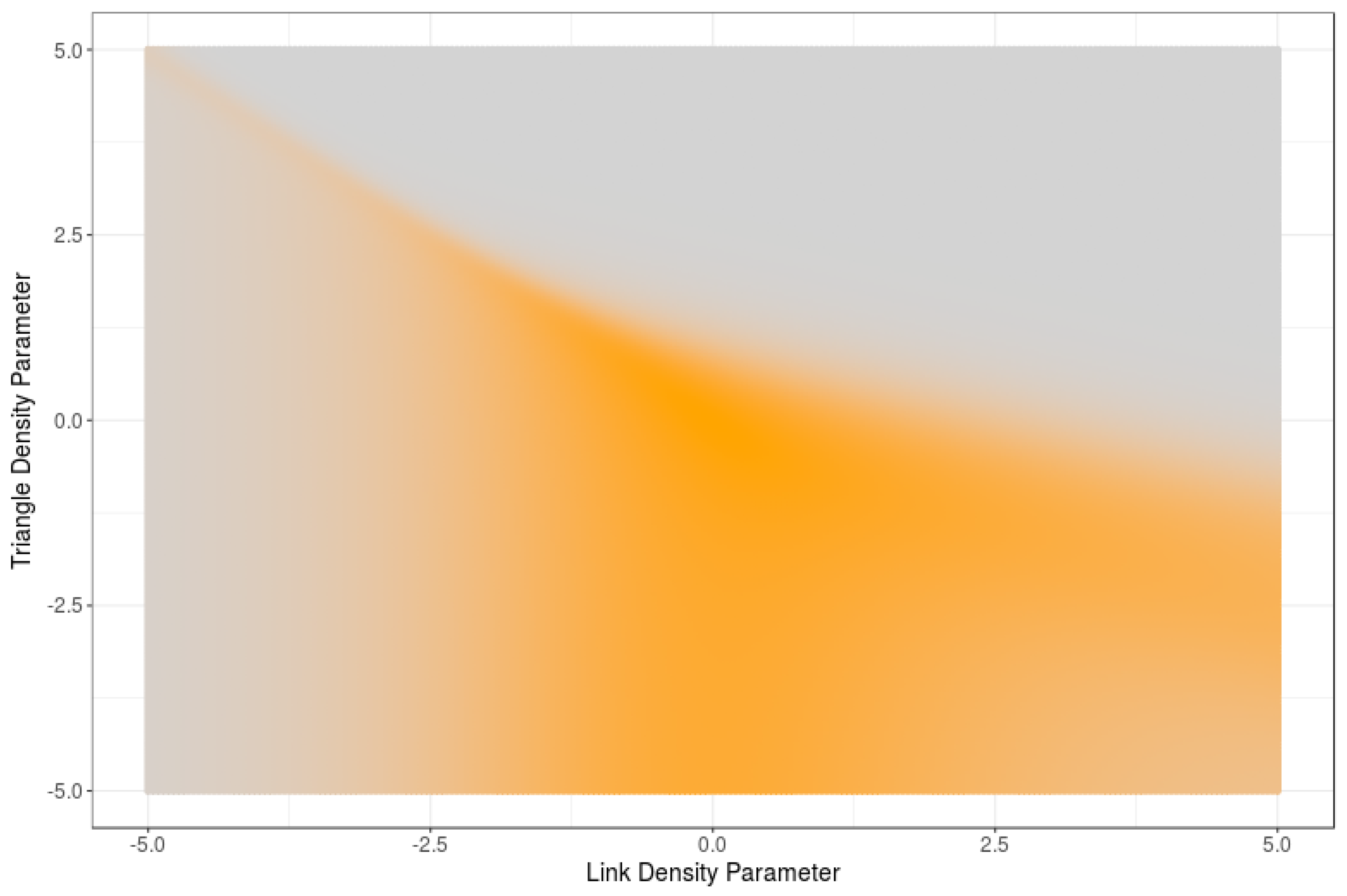
Figure 2.
Average degree entropy of an RNM as a function of link density and triangle density.

Figure 3.
RNM model entropy vs. its average sample degree entropy.
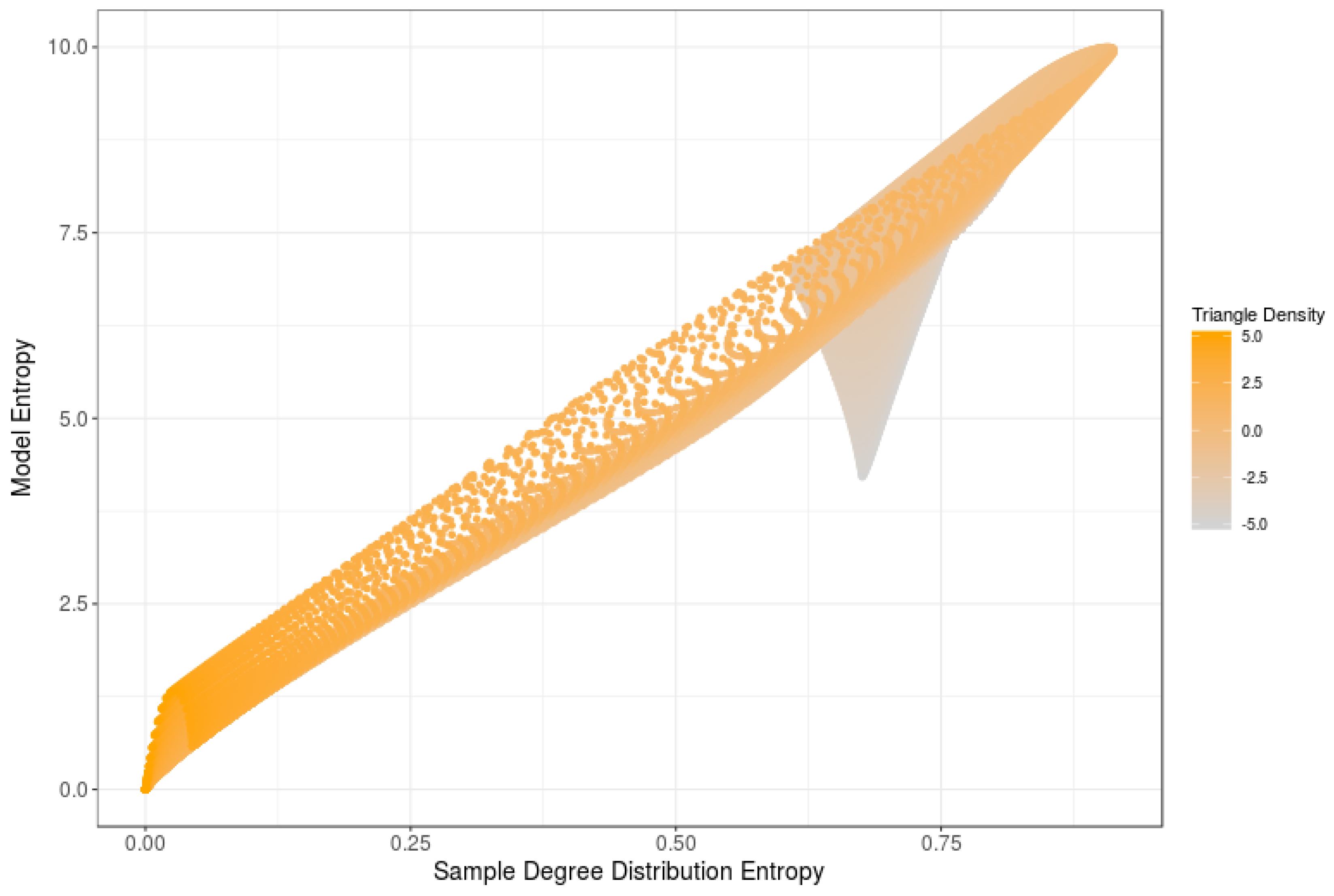
Figure 4.
Connectivity as a function of number of links and number of triangles. Blue = connected; red = not connected.
Figure 4.
Connectivity as a function of number of links and number of triangles. Blue = connected; red = not connected.

© 2017 by the authors. Licensee MDPI, Basel, Switzerland. This article is an open access article distributed under the terms and conditions of the Creative Commons Attribution (CC BY) license (http://creativecommons.org/licenses/by/4.0/).
Share and Cite
MDPI and ACS Style
Zufiria, P.J.; Barriales-Valbuena, I. Entropy Characterization of Random Network Models. Entropy 2017, 19, 321. https://doi.org/10.3390/e19070321
AMA Style
Zufiria PJ, Barriales-Valbuena I. Entropy Characterization of Random Network Models. Entropy. 2017; 19(7):321. https://doi.org/10.3390/e19070321
Chicago/Turabian StyleZufiria, Pedro J., and Iker Barriales-Valbuena. 2017. "Entropy Characterization of Random Network Models" Entropy 19, no. 7: 321. https://doi.org/10.3390/e19070321
Note that from the first issue of 2016, this journal uses article numbers instead of page numbers. See further details here.