Overfitting Reduction of Text Classification Based on AdaBELM
by
 ,
,
Xiaoyue Feng
1 ,
,
Yanchun Liang
1,2,3,
Xiaohu Shi
1,2,
Dong Xu
1,3,
Xu Wang
1 and
Renchu Guan
1,2,* 1
Key Laboratory of Symbolic Computation and Knowledge Engineering of Ministry of Education, College of Computer Science and Technology, Jilin University, Changchun 130012, China
2
Zhuhai Laboratory of Key Laboratory of Symbolic Computation and Knowledge Engineering of Ministry of Education, Zhuhai College of Jilin University, Zhuhai 519041, China
3
Department of Electric Engineering and Computer Science, and Christopher S. Bond Life Sciences Center, University of Missouri, Columbia, MO 65211, USA
*
Author to whom correspondence should be addressed.
Entropy 2017, 19(7), 330; https://doi.org/10.3390/e19070330
Submission received: 2 May 2017
/
Revised: 26 June 2017
/
Accepted: 29 June 2017
/
Published: 6 July 2017
(This article belongs to the Special Issue Information Theory in Machine Learning and Data Science)
Abstract
:Overfitting is an important problem in machine learning. Several algorithms, such as the extreme learning machine (ELM), suffer from this issue when facing high-dimensional sparse data, e.g., in text classification. One common issue is that the extent of overfitting is not well quantified. In this paper, we propose a quantitative measure of overfitting referred to as the rate of overfitting (RO) and a novel model, named AdaBELM, to reduce the overfitting. With RO, the overfitting problem can be quantitatively measured and identified. The newly proposed model can achieve high performance on multi-class text classification. To evaluate the generalizability of the new model, we designed experiments based on three datasets, i.e., the 20 Newsgroups, Reuters-21578, and BioMed corpora, which represent balanced, unbalanced, and real application data, respectively. Experiment results demonstrate that AdaBELM can reduce overfitting and outperform classical ELM, decision tree, random forests, and AdaBoost on all three text-classification datasets; for example, it can achieve 62.2% higher accuracy than ELM. Therefore, the proposed model has a good generalizability.
1. Introduction
The majority of text-classification frameworks employ the vector-space model (VSM), which treats a document as a bag of words and uses plain language words as features [1]. However, this approach uses many redundant features and has a high-dimensional sparse matrix, which potentially leads to overfitting in training and low accuracy in testing [2]. It is obvious that if a learning model excessively pursues the maximization of training accuracy, it can learn a very complex model but fall into overfitting. In this case, rather than “learning” to generalize from a trend, an overfitting model may “memorize” non-predictive features of the training data. For example, Srivastava et al., point out that deep neural networks (DNN) with a large number of parameters are powerful machine learning models but seriously suffer from overfitting [3]. To solve the overfitting problem and pursue better classification performance, several ensemble approaches have been proposed, such as BoosTexter and Bonzaiboost [4,5]. However, the accuracies of these methods are far from being satisfactory and large networks, like DNN, are slow to use, making it difficult to deal with overfitting by combining many different large neural nets [3]. A more successful classification model demands that classification algorithms can more efficiently resolve overfitting and achieve higher accuracy, especially in the era of big data.
Recently, the artificial neural network has garnered much attention, especially in relation to deep learning. Many applications of these deep learning models use feedforward neural network architectures [6]. Feedforward neural networks with random weights can get good performance when the output layer is trained by a single-hidden-layer learning rule or a pseudo-inverse technique [7,8]. The extreme learning machine (ELM) is a single-hidden-layer feedforward network (SLFN), which was proposed by Huang et al. in 2004 [9]. ELM can be considered as a simple framework of random vector functional link networks (RVFL). RVFL is a randomized version of the functional link neural network, where the actual values of the weights from the input layer to the hidden layer can be randomly generated in a suitable domain and kept fixed in the learning stage [10]. However, ELM does not have direct links between the input layer and the output layer and adopts the Moore-Penrose pseudoinverse to obtain the output weights. Compared with traditional computational intelligence techniques and deep learning models, ELM provides a good generalization performance at a faster learning speed with the least amount of human interference [11]. Therefore, it was applied in related fields shortly after it was developed [12,13,14,15,16]. However, for text classification with a high-dimensional sparse matrix, ELM potentially suffers from overfitting because its output weights are solved by the Moore-Penrose generalized inverse, which applies a least-squares minimization [17]. Recently, this drawback of ELM has been analyzed in regression, with models such as the ridge-regression-based ELM and delta test-extreme learning machine (DT-ELM) [17,18,19,20]. Rong et al. and Luo et al. have been noted for their efforts to prune the redundant hidden neurons of ELM for multi-class classification [17,21]. However, in general, pruning methods are rather inefficient because they are used to address larger network structures than necessary in most cases [20].
As an ensemble algorithm, AdaBoost is a fast, simple, and easy-to-use program. It has no parameters to tune (except for the number of iterations) and has been applied to diverse domains with great success, such as in face detection [22], optical character recognition (OCR) problems [23], and vehicle classification [24]. More importantly, it is often empirically resistant to overfitting and achieves excellent performance on both benchmark datasets and real applications [25,26,27]. Meanwhile, AdaBoost is equipped with a set of theoretical guarantees. In 2003, Schapire and Freund won the Gödel Prize, which is the most prestigious award in theoretical computer science, based on their theoretical contribution [28] to AdaBoost. Attempts to solve the interesting mystery about why boosting methods do not overfit has generated debates between margin theory and the statistical perspective, which have continued for the past 20 years [27,29,30,31,32]. Recently, Zhou et al. proved sharper bounds and provided an answer to Breiman’s doubt about the margin theory [26,27].
In this paper, we first analyze the overfitting problem in classification, especially in text mining. Different from the hidden-neuron pruning strategy, we propose a novel text classification algorithm, which introduces AdaBoost to reduce overfitting without modifying the framework of ELM. In addition, to validate the performance of the proposed algorithm, the classical ELM [11], decision tree [5], random forests (RF) [33,34], oblique random forests (oRF) [35,36], and the AdaBoost [5] algorithm are compared on balanced, unbalanced, and real-application datasets. There are three main contributions in our approach: (1) the new AdaBELM model is proposed, which reduces overfitting of ELM and achieves higher classification accuracy, (2) a novel rate of overfitting (RO) is proposed, which can be used to analyze overfitting quantitatively, and (3) the proposed algorithm is shown to have good generalizability against balanced, unbalanced and real datasets.
The remainder of this paper is organized as follows. A brief analysis of AdaBoost and the extreme learning machine algorithm is given in Section 2. Section 3 describes the overfitting problem, and Section 4 proposes the AdaBELM model in detail. Section 5 presents the experimental framework and results. Finally, Section 6 draws a conclusion from our work.
2. Related Work
2.1. Extreme Learning Machine
The extreme learning machine offers advantages such as fast learning speed, ease of implementation, and minimal human intervention [13]. Different from the traditional artificial neural networks trained with slow, gradient-based learning algorithms and deep neural networks with many parameters that require tuning, ELM can provide good performance at an extremely fast learning speed [11]. In theory, this algorithm is derived from single-hidden-layer feedforward neural networks (SLFN), which randomly choose hidden nodes and determine the output weights of SLFN. In other words, the parameters related to the hidden nodes are randomly assigned but not tuned in training steps. Therefore, in the procedure of determining network parameters, iteration is not needed and the time for adjusting parameters evidently decreases. Optimization of the weights in the output layer is carried out using a Moore–Penrose generalized inverse [37].
After Huang et al. proposed the ELM algorithm, it was applied widely in computational intelligence and machine learning [11,12,13,14,15,16]. However, ELM may cause overfitting when it computes an output for high-dimensional data. In other words, a network that is too large could overfit the training data, thus producing poor generalization performance on unseen cases. Moreover, a larger network also leads to a longer prediction-response time and more requirements for memory, as well as hardware implementation [21].
2.2. AdaBoost
The origin of the AdaBoost algorithm can be traced back to a well-known question proposed by Kearns and Valiant concerning probably approximately correct (PAC) learning and machine learning. In 1988, Kearns and Valiant (Turing Award Winners for their work on PAC learning) proposed that a weak learning algorithm could be “boosted” into an arbitrarily accurate strong learning algorithm [38]. Two years later, Schapire worked out a constructive proof, which was the first boosting algorithm [39]. As an iterative algorithm, it needs no prior knowledge about the accuracy of the hypotheses of the weak learning algorithm.
The main procedure of AdaBoost is described as follows. Initially, the training samples are all given the same weight; this set of equal weights is denoted as D1. Second, the distribution of the weights is denoted at the t-th iteration as Dt, and weak classifiers ht: X → Y are generated from the training set and Dt. The error rate of ht can be calculated. Then, the weights of the samples that are not correctly classified will be increased, and the weights of those that are correctly classified will be decreased. The new weights of the samples Dt+1 will be adopted in the next iteration. From the training set and Dt+1, another base learner will be generated. Such a process is repeated for T iterations. The final model is achieved by weighted majority voting of the T weak learners, where the weights of the learners are computed during the training process [23,38]. The algorithm is named AdaBoost because it adaptively adjusts to the errors of the weak hypotheses returned by weak classifiers. The framework of AdaBoost’s training process is shown in Algorithm 1.
| Algorithm 1. AdaBoost Algorithm. |
| Input: Training data set D = {(x1,y1),…,(xm, ym)}; Ensemble size T; |
| Output: |
Procedure:
|
3. A Quantitative Measurement for Overfitting
Overfitting (i.e., high variance) is an important issue in machine learning, especially for supervised learning algorithms. To rigorously describe the overfitting problem for classification, we proposed a quantitative measurement, rate of overfitting, denoted as RO:
where y and z indicate the testing error and the training error, respectively. Parameter u could be the training size or iteration time. In this paper, the former is used in our experiments. The sign of RO is decided by the testing error. When RO is less than 0, it means that with the training set increasing, the testing error also goes up.And the smaller the value of RO, the worse the overfitting. To keep the testing error y going down and avoid overfitting, some algorithms may enlarge the training error z by adding penalty into the objective function. When RO equals to 0, it means that with the training set increases, testing error does not change any more. When RO is larger than 0, it means the testing error y is decreasing. If the value of RO remains positive, it means that the model has not fallen into overfitting. Using this measurement, we can consider the training and testing error simultaneously and comprehensively.
To clearly explain the overfitting problem, we list the results of ELM, Gini Tree, and Bonzaiboost (a new and powerful AdaBoost algorithm for text classification [5]), random forests, and oblique random forests in Table 1 and Table 2. The random forests method is similar with the ensemble learning. It is a combination of tree predictors such that each tree depends on the values of a random vector sampled independently and with the same distribution for all trees in the forest [34]. Fernández-Delgado et al. compared 179 classifiers arising from 17 families and determined that the random forests method achieves the best performance for any dataset [33]. Oblique random forests, as an ensemble method transforms the data at each node to another space when computing the best split at this node [35,36]. We use classification and regression tree (CART) as the base classifier, and choose two kinds of transformation methods for comparison, namely that linear discriminate analysis (LDA) and the multisurface proximal support vector machine (MPSVM). They are denoted as LDA-RF and MPSVM-RF in the text below. From Table 1 and Table 2, we can see the following two results: (1) When an ELM training error rate of zero has already been achieved in Table 1, the testing error is still changing. As the size of the training data set increases, the error rate of the testing rises, from 0.64 against 20% of the 20 Newsgroups training data (11,314 samples in total) to 0.66 on 40% of the training data. Then, after a decrease to 0.50 against 60% of the training data, it increases again to 0.57 and 0.58 for 80% and 100% of the training data, respectively. (2) In Table 2, the overfitting phenomenon is much easier to recognize. According to our explanation of the RO, when its value is less than 0, the model falls into overfitting. With the RO measurement, i.e., Equation (1), we find that the RO values of ELM are −0.09, −0.37, and −0.06 against 40%, 80%, and 100% of the training data, respectively. Therefore, ELM exhibits high variance. The Gini Tree also falls into overfitting on 80% of the training data, as indicated by the −0.03 RO value.
Comparing RO with the error rate, we can find that RO is easier to use than the error rate to assess the overfitting problem. Moreover, the RO value can further describe the level of overfitting quantitatively. For example, the RO value of ELM is −0.37 on 80% of the training data, which indicates that its overfitting problem is more serious than on 40% of the training data, with an RO value of −0.09.
To overcome the problem associated with overfitting, Deng et al. proposed a regularized ELM to relieve the overfitting problem by penalizing the training error [40]. However, to maintain comparable accuracy, it usually requires a much larger number of hidden neurons and hence a very complicated network is generated [16,40]. A kernel ELM with better generalizability was also proposed, in which the single hidden layer does not need to be neuron-like [41]. However, the computational cost and the required memory needed to calculate the inverse of the regularized square matrix make it a great challenge to address large-scale data. Luo et al. proposed a sparse Bayesian ELM for multi-classification. However, since it was originally derived from binary classification, it has to use the pairwise coupling in the multi-classification extension [17]. When facing many classes (for example, more than 50), its classification effectiveness and efficiency will go down quickly. Thus, improvement is needed for conventional ELM to efficiently solve the overfitting problem in text multi-classification.
4. AdaBoost ELM Model
Let X be a set of N samples (text in our case) and Y serve as the set of class labels. A training set D = {(x1, y1), (x2, y2) ,…, (xm, ym)} is given, where xi ∈ X, yi ∈ Y = {1,2,…,C} (i = 1,…,m) and C is the number of classes. Standard SLFN with K nodes are mathematically modeled by:
where wk represents the parameters of the k-th element of the hidden layer, such as weights and biases of the multilayer perceptron; hk is the weight that connects the k-th hidden element with the output layer; and f is the activation function of the hidden layer. In matrix notation, Equation (2) can be expressed as O = Fh, where h is the vector of the output-layer weights, and F is represented as
where K is the number of hidden nodes. ELM uses a random initialization of the parameters of the hidden layer, and the weights of the output layer in h are calculated using the Moore-Penrose generalized inverse as follows:
where F† is the pseudo-inverse matrix of F, and the superscript T indicates transposition [17,37]. Finally, the predicted class label of sample xi is:
and j is the j-th node of the output layer.
h = F†O, F† = (FT F)−1 FT
In the context of experiments, the generalization error of the ensemble learners continues to decrease as the training data size increases, even after the training error has reached zero. Therefore, to reduce the overfitting problem and achieve high performance on multi-class text classification, we designed a novel model based on AdaBoost, which is called AdaBELM. The flowchart of the AdaBELM model is shown in Figure 1. It introduces the AdaBoost framework used to boost ELM. A damping factor λ (0 < λ ≤ 1) is defined to control the ensemble scale. Hence, when 0 < λ < 1, AdaBELM selects a subset of the training samples for each ELM; thus, when λ = 1, it uses the whole set of training data. This idea is borrowed from the stochastic gradient-descent algorithm, which is used to solve large-scale linear prediction problems [42]. For the selection of a training subset, we employ roulette sampling. Using this method, AdaBELM can handle the big-data problem accordingly.
With the highly efficient base learner ELM, AdaBELM can quickly achieve a good classifier. Moreover, AdaBoost can continue to decrease the testing error as its training data size increases, even after the training error has reached zero (see Table 1), which means our AdaBELM model can reduce the overfitting problem under the AdaBELM framework as shown in Algorithm 2.
| Algorithm 2. AdaBELM Algorithm. |
| Input: Training data set D = {(x1,y1),…,(xm, ym)}; Ensemble size T; |
| Output: |
Procedure:
|
Compared with classical AdaBoost, which uses the whole training set D, AdaBELM uses the subset D′ to train the base classifier with a sampling strategy (see step 3 in Algorithm 2). Some of the training data that have not been sampled will be calculated in step 5 in the diagram. Consequently, when updating the weights for samples (see step 7 in Algorithm 2), the unsampled and error data are going to be assigned higher weights in the next round of learning.
5. Experiments and Discussion
To evaluate the performance of the proposed model, AdaBELM, three datasets and classical algorithms, including Gini Tree (C4.5), random forests [33], oblique random forests [35,36], Bonzaiboost (AdaBoost.MH) [5], and extreme learning machine [11], were employed for comparison. Hereinto, random forests, oblique random forests, Bonzaiboost, and AdaBELM are ensemble models, which employ CART, CART, Gini Tree, and ELM as base learners, respectively.
5.1. Datasets
We selected three benchmark text data sets, namely 20 Newsgroups, Reuters-21578, and BioMed. The first has a uniform distribution and the second has an unbalanced distribution. The third dataset, the BioMed corpora, is a collection of BioMed scientific publications. BioMed consists of a full text of scientific papers, while Reuters and 20 Newsgroups contain only short documents. The details of these data are as follows.
- 20 Newsgroups is a widely used benchmark dataset. It was first collected by Ken Lang and partitioned evenly in 20 different newsgroups [43]; some of the classes are very closely related to one another (e.g., comp.sys.ibm.pc.hardware and comp.sys.mac.hardware) and others are highly unrelated (e.g., misc.forsale and soc.religion.christian). There are three versions, i.e., “20news-19997,” “20news-bydate”, and “20news-18828”; however, we used the “20news-bydate” version. It is recommended by the data provider since the label information has been removed, and the training and testing sets are separated in time, which makes it more realistic.
- Reuters-21578 (Reuters) is a publicly available benchmark text data set, which has been manually pre-classified [37]. The original Reuters data consist of 22 files (a total of 21,578 documents) and contain special tags such as “<TOPICS>” and “<DATE>”, among others. The pre-processing phase on the dataset cuts the files into single texts and strips the document of the special tags. We selected the public available ModApte version from http://www.cad.zju.edu.cn/home/dengcai/Data/TextData.html in our experiment [44]. Compared with 20 Newsgroups, Reuters is more difficult to classify [45]. Each class has a wider variety of documents, and these classes are much more unbalanced. For example, the largest category (“earn”) contains 3713 documents, while some small categories, such as “naphtha”, contains only one document. To determine the robustness of the unbalanced data sets, we used 65 categories, and the number of documents in each category ranges from 2 to 3713.
- BioMed corpora is a BioMed central open-access corpora dataset. From the BioMed corpora, 110,369 articles from January 2012 to June 2012 were downloaded. During the pre-processing phase, small files contain only XML tags (such as <title> and <body>) and those less than 4 KB were removed. Then, the data was divided into different “topics” based on journal names and the top 10 topics (each included in from 1966 to 5022 articles) were selected as the experimental corpora. Stop words and journal-name information were eliminated from the text. Then, each document is represented by a superset of two-tuples as follows:where N is the number of documents in the data set; Mj is the number of term features (unique words or phrases) in the j-th document; di = {<fi1, ni1>, <fi2, ni2>,…, <fiMi, niMi>} refers to the i-th document, and fik and nik represent the k-th term in the i-th document and its frequency, respectively.
From Table 3, we can see the following: (1) The sparsity rates of all three datasets are high (>98%), which indicates that all of them will lead to a high-dimensional sparse problem. (2) Compared with the discrete uniform distributions of 20 Newsgroups and BioMed, Reuters has a much more non-uniform distribution of data according to the “max and min class sizes” in Table 3; hence, it is more difficult to classify than the other two.
5.2. Experimental Results
First, the overfitting problem should be discussed according to the comparisons between Table 1 and Table 4 (see Section 3). From these comparisons, we can safely draw the following conclusions. First, the error rate of ELM increases as the size of the training set increases. As previously mentioned, ELM suffers from an overfitting problem. Because this is a high-dimensional sparse problem, ELM must learn a large and complex network. By introducing the AdaBoost framework, the proposed AdaBELM algorithm overcomes this problem. The gap between the testing and training errors of AdaBELM narrows, while the training set margin of error widens.
Moreover, from Table 5, we can see that all the RO values (computed according to Equation (1)) of AdaBELM are above zero. Benefiting from AdaBoost, AdaBELM easily avoids two decreases that would certainly be induced from ELM overfitting. In addition, the training errors of AdaBELM are similar with those of ELM, all of which are close to zero. In contrast, the training error of Bonzaiboost (AdaBoost) increases to 0.08 with an increasing size of the set of training data. AdaBELM obtains the lowest error rates while its training error is close to zero. In other words, AdaBELM not only reduces the overfitting problem but also achieves the highest accuracy.
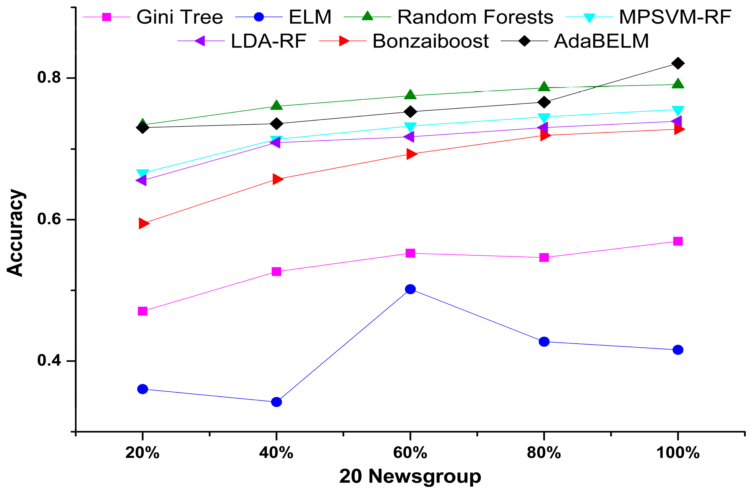
From the trends of these learning curves in Figure 2, it is evident that the new hybrid model AdaBELM achieves the highest accuracy among the seven algorithms. Bonzaiboost (AdaBoost) continually improves its accuracies with the increase of the number of training samples, and ELM falls behind due to overfitting. In addition, from Figure 2, ELM performs worse than Gini Tree; however, our newly proposed model, AdaBELM, using ELM as the base learner, is superior to Bozaiboost based on Gini Tree.
Moreover, to examine the performance and robustness of the proposed algorithms, the seven algorithms’ results on the three benchmark corpora are compared, as shown in Table 6. AdaBELM achieves the highest accuracy among the seven algorithms on all three datasets. For example, on Reuters-21578, the accuracy of AdaBELM reaches 0.88 and is 2.74%, 7.3%, 11.2%, 23.7%, 9.10%, and 5.26% higher than Bonzaiboost (AdaBoost), random forests, MPSVM-RF, LDA-RF, Gini tree, and ELM, respectively. On the BioMed corpora, its accuracy reaches 0.88, which is 2.13%, 24.63% and 62.20% higher than Bonzaiboost (AdaBoost), Gini tree and ELM, respectively. The next-best models on the three different datasets are Bonzaiboost and three random forests. For instance, the classical random forests can achieve 0.88 accuracy which is the same as AdaBELM. As a result of employing ensemble strategies, four boosts base classifiers (decision trees) improved the classification accuracy and achieved the second position. The performance rankings of the remaining two algorithms were inconsistent on the three datasets. For example, ELM obtained an accuracy of 0.84, which is 3.76% higher than the Gini Tree on Reuters. However, the Gini Tree obtained a better result than ELM on 20 Newsgroups. In addition, to guarantee generalizability for those random initiation algorithms, we ran each program 10 times for each algorithm and all the accuracies were averages of these results.
There are two parameters in the proposed model: One is the number of hidden-layer neurons N, and the other is the number of base learners T (ELM in our case and Gini Tree for Bonzaiboost). Because the number of hidden-layer neurons is important for feedforward neural networks, many experiments were conducted to select the numbers of hidden-layer neurons for ELM and AdaBELM. We chose the number of hidden-layer neurons with which the highest value of the training accuracy was attained. For ELM, we chose 3200, 6300, and 500 for the Reuters-21578, 20 Newsgroups and BioMed corpora, respectively. For the sake of fairness, AdaBELM used the same selection method, with which 1900, 3500, and 290 were selected.
After determining the number of hidden-layer neurons for each dataset, the number of base learners (ELM in our case, Gini Tree for Bonzaiboost) should be selected. Considering time and space complexities, which are of great importance for the AdaBoost algorithm, both algorithms adopted 200 base learners on the three data sets. Random Forests chose 500 as the tree number. MPSVM-RF and LDA-RF chose 100 as the tree number. We set the damping factor λ of AdaBELM (0 < λ ≤ 1) as 0.8, which can be selected according to different data, applications and computing resources. When facing big data with limited memory, a smaller value of λ should be selected, and a larger value should be specified for small data with sufficient memory.
6. Conclusions
In this paper, to clearly quantify the overfitting problem, we defined a new measurement called the rate of overfitting (RO). To reduce the overfitting problem and pursue high performance on text classification, we proposed a novel algorithm, AdaBELM. Using the proposed quantitative measurement, we found that the RO of ELM decreased to below zero three times. This means that ELM suffers from a significant overfitting problem, which is due to the output weights being computed by the Moore-Penrose generalized inverse, which is a least-squares minimization issue. However, the proposed model AdaBELM not only reduced this drawback, but also achieved the highest accuracy when compared (and tested) with random forests, oblique random forests, Bonzaiboost (AdaBoost MH), Gini Tree, and traditional ELM using the same parameters. Moreover, the comparisons among Reuters-21578, 20 Newsgroups, and BioMed revealed that the results of the new model are also superior to those of the other four algorithms. In other words, the proposed model has good generalizability, as revealed by its high performance on balanced, unbalanced, and real application data.
Acknowledgments
The authors are grateful for the support of the National Natural Science Foundation of China (61602207, 61572228, 61472158, 61373050), the Science Technology Development Project from Jilin Province (20160101247JC), the Zhuhai Premier Discipline Enhancement Scheme, the Guangdong Premier Key-Discipline Enhancement Scheme, the Educational Commission of Jilin Province, and the China Scholarship Council.
Author Contributions
Xiaoyue Feng and Renchu Guan conceived and designed the experiments; Xiaoyue Feng and Xu Wang performed the experiments; and Yanchun Liang, Xiaohu Shi, and Dong Xu reviewed the paper and provided suggestions. All authors have read and approved the final manuscript.
Conflicts of Interest
The authors declare no conflict of interest.
References
- Sebastiani, F. Machine Learning in Automated Text Categorization. ACM Comput. Surv. 2002, 34, 1–47. [Google Scholar] [CrossRef]
- Joachims, T. Text Categorization with Support Vector Machines: Learning with Many Relevant Features; Springer: Berlin/Heidelberg, Germany, 1998; pp. 137–142. [Google Scholar]
- Srivastava, N.; Hinton, G.; Krizhevsky, A.; Sutskever, I.; Salakhutdinov, R. Dropout: A Simple Way to Prevent Neural Networks from Overfitting. J. Mach. Learn. Res. 2014, 15, 1929–1958. [Google Scholar]
- Schapire, R.E.; Singer, Y. BoosTexter: A Boosting-based System for Text Categorization. Mach. Learn. 2000, 39, 135–168. [Google Scholar] [CrossRef]
- Laurent, A.; Camelin, N.; Raymond, C. Boosting Bonsai Trees for Efficient Features Combination: Application to Speaker Role Identification. In Proceedings of the 15th Annual Conference of the International Speech Communication Association, Singapore, 12 March 2014; pp. 76–80. [Google Scholar]
- LeCun, Y.; Bengio, Y.; Hinton, G. Deep Learning. Nature 2015, 521, 436–444. [Google Scholar] [CrossRef] [PubMed]
- Igelnik, B.; Pao, Y.H. Stochastic Choice of Basis Functions in Adaptive Function Approximation and The Functional-Link Net. IEEE Trans. Neural Netw. 1995, 6, 1320–1329. [Google Scholar] [CrossRef] [PubMed]
- Pao, Y.H.; Takefuji, Y. Functional-link Net Computing: Theory, System Architecture, and Functionalities. Computer 1992, 25, 76–79. [Google Scholar] [CrossRef]
- Huang, G.B.; Zhu, Q.Y.; Siew, C.K. Extreme Learning Machine: A New Learning Scheme of Feedforward Neural Networks. In Proceedings of the 2004 IEEE International Joint Conference on Neural Networks, Budapest, Hungary, 25–29 July 2004; pp. 985–990. [Google Scholar]
- Zhang, L.; Suganthan, P.N. A comprehensive evaluation of random vector functional link networks. Inf. Sci. 2016, 367, 1094–1105. [Google Scholar] [CrossRef]
- Huang, G.B.; Zhu, Q.Y.; Siew, C.K. Extreme Learning Machine: Theory and Applications. Neurocomputing 2006, 70, 489–501. [Google Scholar] [CrossRef]
- Extreme Learning Machines: Random Neurons, Random Features, Kernels. Available online: http://www.ntu.edu.sg/home/egbhuang/ (accessed on 16 March 2017).
- Huang, G.B.; Wang, D.H.; Lan, Y. Extreme Learning Machines: A Survey. Int. J. Mach. Learn. Cybern. 2011, 2, 107–122. [Google Scholar] [CrossRef]
- Miche, Y.; Sorjamaa, A.; Bas, P.; Simula, O.; Jutten, C.; Lendasse, A. OP-ELM: Optimally Pruned Extreme Learning Machine. IEEE Trans. Neural Netw. 2010, 21, 158–162. [Google Scholar] [CrossRef] [PubMed]
- Soria-Olivas, E.; Gomez-Sanchis, J.; Martin, J.D.; Vila-Frances, J.; Martinez, M.; Magdalena, J.R.; Serrano, A.J. BELM: Bayesian Extreme Learning Machine. IEEE Trans. Neural Netw. 2011, 22, 505–509. [Google Scholar] [CrossRef] [PubMed]
- Choi, K.; Toh, K.A.; Byun, H. Realtime Training on Mobile Devices for Face Recognition Applications. Pattern Recognit. 2011, 44, 386–400. [Google Scholar] [CrossRef]
- Luo, J.; Vong, C.M.; Wong, P.K. Sparse Bayesian Extreme Learning Machine for Multi-classification. IEEE Trans. Neural Netw. Learn. Syst. 2014, 25, 836–843. [Google Scholar] [PubMed]
- Neumann, K.; Steil, J.J. Optimizing Extreme Learning Machines via Ridge Regression and Batch Intrinsic Plasticity. Neurocomputing 2013, 102, 23–30. [Google Scholar] [CrossRef]
- Er, M.J.; Shao, Z.; Wang, N. A Fast and Effective Extreme Learning Machine Algorithm Without Tuning. In Proceedings of the 2014 International Joint Conference on Neural Networks (IJCNN), Beijing, China, 6–11 July 2014; pp. 770–777. [Google Scholar]
- Yu, Q.; van Heeswijk, M.; Miche, Y.; Nian, R.; He, B.; Séverin, E.; Lendasse, A. Ensemble Delta Test-Extreme Learning Machine (DT-ELM) for Regression. Neurocomputing 2014, 129, 153–158. [Google Scholar] [CrossRef]
- Rong, H.J.; Ong, Y.S.; Tan, A.H.; Zhu, Z. A Fast Pruned-Extreme Learning Machine for Classification Problem. Neurocomputing 2008, 72, 359–366. [Google Scholar] [CrossRef]
- Viola, P.; Jones, M. Rapid Object Detection Using a Boosted Cascade of Simple Features. In Proceedings of the 2001 IEEE Computer Society Conference on Computer Vision and Pattern Recognition, CVPR 2001, Kauai, HI, USA, 8–14 December 2001; pp. 511–518. [Google Scholar]
- Freund, Y.; Schapire, R.E. Experiments with A New Boosting Algorithm. In Proceedings of the 13th International Conference of machine learning, Bari, Italy, 2 January 1996; pp. 148–156. [Google Scholar]
- Wen, X.; Shao, L.; Xue, Y.; Fang, W. A Rapid Learning Algorithm for Vehicle Classification. Inf. Sci. 2015, 295, 395–406. [Google Scholar] [CrossRef]
- Bauer, E.; Kohavi, R. An Empirical Comparison of Voting Classification Algorithms: Bagging, Boosting, and Variants. Mach. Learn. 1999, 36, 105–139. [Google Scholar] [CrossRef]
- Dietterich, T.G. An Experimental Comparison of Three Methods for Constructing Ensembles of Decision Trees: Bagging, Boosting, and Randomization. Mach. Learn. 2000, 40, 139–157. [Google Scholar] [CrossRef]
- Gao, W.; Zhou, Z.H. On the Doubt About Margin Explanation of Boosting. Artif. Intell. 2013, 203, 1–18. [Google Scholar] [CrossRef]
- Freund, Y.; Schapire, R.E. A Desicion-Theoretic Generalization of On-Line Learning and an Application to Boosting; Springer: Berlin/Heidelberg, Germany, 1995; pp. 23–37. [Google Scholar]
- Grove, A.J.; Schuurmans, D. Boosting in the Limit: Maximizing the Margin of Learned Ensembles. In Proceedings of the 15th National Conference on Artificial Intelligence, Madison, WI, USA, 26–30 July 1998. [Google Scholar]
- Rätsch, G.; Onoda, T.; Müller, K.R. Soft Margins for AdaBoost. Mach. Learn. 2001, 42, 287–320. [Google Scholar] [CrossRef]
- Reyzin, L.; Schapire, R.E. How Boosting the Margin Can Also Boost Classifier Complexity. In Proceedings of the 23rd International Conference on Machine Learning, New York, NY, USA; 2006; pp. 753–760. [Google Scholar]
- Audibert, J.Y.; Munos, R.; Szepesvári, C. Exploration–Exploitation Tradeoff Using Variance Estimates in Multi-Armed Bandits. Theor. Comput. Sci. 2009, 410, 1876–1902. [Google Scholar] [CrossRef]
- Fernández-Delgado, M.; Cernadas, E.; Barro, S.; Amorim, D. Do we Need Hundreds of Classifiers to Solve Real World Classification Problems? J. Mach. Learn. Res. 2014, 15, 3133–3181. [Google Scholar]
- Breiman, L. Random Forests. Mach. Learn. 2001, 45, 5–32. [Google Scholar] [CrossRef]
- Zhang, L.; Suganthan, P.N. Oblique Decision Tree Ensemble via Multisurface Proximal Support Vector Machine. IEEE Trans. Cybern. 2015, 45, 2165–2176. [Google Scholar] [CrossRef] [PubMed]
- Zhang, L.; Suganthan, P.N. Random forests with ensemble of feature spaces. Pattern Recognit. 2014, 47, 3429–3437. [Google Scholar] [CrossRef]
- Rao, C.R.; Mitra, S.K. Generalized Inverse of a Matrix and Its Applications. Berkeley Symp. Math. Stat. Probab. 1972, 1, 601–620. [Google Scholar]
- Wu, X.; Kumar, V.; Quinlan, J.R.; Ghosh, J.; Yang, Q.; Motoda, H.; McLachlan, G.J.; Ng, A.; Liu, B.; Yu, P.S.; et al. Top 10 Algorithms in Data Mining. Knowl. Inf. Syst. 2008, 14, 1–37. [Google Scholar] [CrossRef]
- Schapire, R.E. The Strength of Weak Learnability. Mach. Learn. 1990, 5, 197–227. [Google Scholar] [CrossRef]
- Deng, W.; Zheng, Q.; Chen, L. Regularized Extreme Learning Machine. In Proceedings of the 2009 IEEE Symposium on Computational Intelligence and Data Mining, Nashville, TN, USA, 30 March–2 April 2009; pp. 389–395. [Google Scholar]
- Zhang, T. Solving Large Scale Linear Prediction Problems Using Stochastic Gradient Descent Algorithms. In Proceedings of the Twenty-First International Conference on Machine Learning, New York, NY, USA, 4–8 July 2004; p. 116. [Google Scholar]
- Huang, G.B.; Zhou, H.; Ding, X.; Zhang, R. Extreme Learning Machine for Regression and Multiclass Classification. IEEE Trans. Syst. Man Cybern. Part B Cybern. 2012, 42, 513–529. [Google Scholar] [CrossRef] [PubMed]
- Home Page for 20 Newsgroups Data Set. Available online: http://qwone.com/~jason/20Newsgroups/ (accessed on 17 March 2017).
- Cai, D.; He, X.; Han, J. Document Clustering Using Locality Preserving Indexing. IEEE Trans. Knowl. Data Eng. 2005, 17, 1624–1637. [Google Scholar] [CrossRef]
- Guan, R.; Shi, X.; Marchese, M.; Yang, C.; Liang, Y. Text Clustering with Seeds Affinity Propagation. IEEE Trans. Knowl. Data Eng. 2011, 23, 627–637. [Google Scholar] [CrossRef]
Figure 1.
Flowchart of AdaBELM.
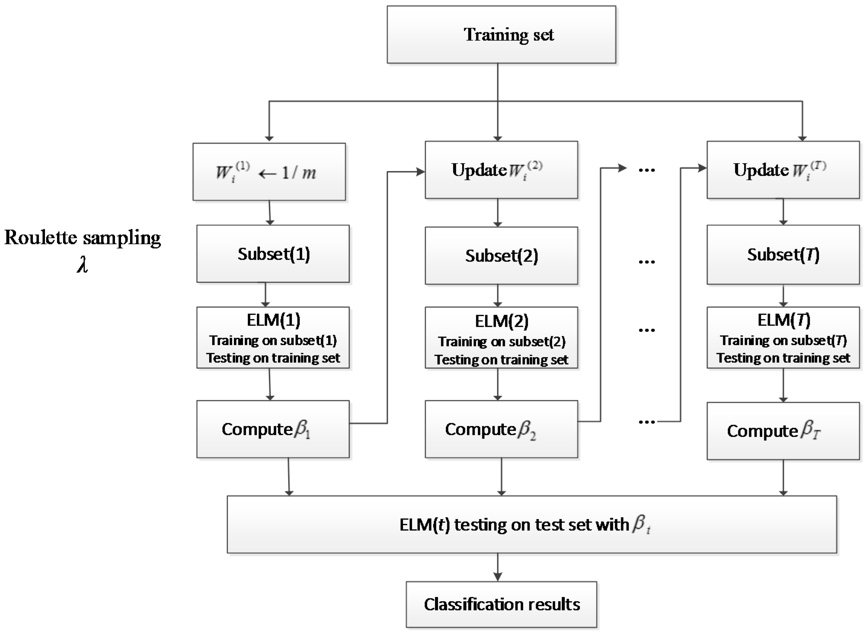
Figure 2.
Accuracy comparisons for Gini Tree, ELM, random forests, oblique random forests (MPSVM-RF, LDA-RF), Bonzaiboost and AdaBELM on five different percentages of a 20 Newsgroups training set.
Figure 2.
Accuracy comparisons for Gini Tree, ELM, random forests, oblique random forests (MPSVM-RF, LDA-RF), Bonzaiboost and AdaBELM on five different percentages of a 20 Newsgroups training set.


Table 1.
Error rate comparison of Gini Tree, ELM, random forests, oblique random forests (MPSVM-RF, LDA-RF), and Bozaiboost on 20 Newsgroups.
Table 1.
Error rate comparison of Gini Tree, ELM, random forests, oblique random forests (MPSVM-RF, LDA-RF), and Bozaiboost on 20 Newsgroups.
| Data Scale | 20% | 40% | 60% | 80% | 100% | |||||
|---|---|---|---|---|---|---|---|---|---|---|
| Training | Testing | Training | Testing | Training | Testing | Training | Testing | Training | Testing | |
| Gini Tree | 0.00 | 0.53 | 0.00 | 0.47 | 0.00 | 0.45 | 0.00 | 0.45 | 0.00 | 0.43 |
| ELM | 0.00 | 0.64 | 0.00 | 0.66 | 0.00 | 0.50 | 0.00 | 0.57 | 0.00 | 0.58 |
| Random Forests | 0.00 | 0.26 | 0.00 | 0.24 | 0.00 | 0.22 | 0.00 | 0.21 | 0.00 | 0.21 |
| MPSVM-RF | 0.02 | 0.33 | 0.02 | 0.29 | 0.02 | 0.27 | 0.02 | 0.25 | 0.02 | 0.25 |
| LDA-RF | 0.02 | 0.35 | 0.02 | 0.29 | 0.02 | 0.71 | 0.02 | 027 | 0.02 | 0.26 |
| Bonzaiboost | 0.00 | 0.41 | 0.02 | 0.34 | 0.05 | 0.31 | 0.07 | 0.28 | 0.08 | 0.27 |
Table 2.
RO Comparisons of Gini Tree, ELM, random forests, oblique random forests (MPSVM-RF, LDA-RF), and Bonzaiboost on 20 Newsgroups; negative ROs are in bold.
Table 2.
RO Comparisons of Gini Tree, ELM, random forests, oblique random forests (MPSVM-RF, LDA-RF), and Bonzaiboost on 20 Newsgroups; negative ROs are in bold.
| Data Scale | 40% | 60% | 80% | 100% |
|---|---|---|---|---|
| Gini Tree | 0.28 | 0.15 | −0.03 | 0.12 |
| ELM | −0.09 | 0.80 | −0.37 | −0.06 |
| Random Forests | 0.13 | 0.07 | 0.06 | 0.02 |
| MPSVM-RF | 0.23 | 0.09 | 0.06 | 0.05 |
| LDA-RF | 0.24 | 0.03 | 0.08 | 0.05 |
| Bonzaiboost | 0.28 | 0.15 | 0.12 | 0.04 |
Table 3.
Basic information of the three datasets.
| Data Sets | Reuters-21578 | 20 Newsgroups | Biomed |
|---|---|---|---|
| No. text | 8293 | 18,846 | 1000 |
| No. classes | 65 | 20 | 10 |
| Max. class size | 3713 | 600 | 100 |
| Min. class size | 2 | 377 | 100 |
| Avg. class size | 127.58 | 942.30 | 100 |
| Number of features | 18,933 | 61,188 | 69,601 |
| Sparsity rate (“0”/all) | 99.77% | 99.73% | 98.85% |
Table 4.
Error rate comparison of Gini Tree, ELM, random forests, oblique random forests (MPSVM-RF, LDA-RF), Bozaiboost and AdaBELM on 20 Newsgroups.
Table 4.
Error rate comparison of Gini Tree, ELM, random forests, oblique random forests (MPSVM-RF, LDA-RF), Bozaiboost and AdaBELM on 20 Newsgroups.
| Data Scale | 20% | 40% | 60% | 80% | 100% | |||||
|---|---|---|---|---|---|---|---|---|---|---|
| Training | Testing | Training | Testing | Training | Testing | Training | Testing | Training | Testing | |
| Gini Tree | 0.00 | 0.53 | 0.00 | 0.47 | 0.00 | 0.45 | 0.00 | 0.45 | 0.00 | 0.43 |
| ELM | 0.00 | 0.64 | 0.00 | 0.66 | 0.00 | 0.50 | 0.02 | 0.57 | 0.02 | 0.58 |
| Random Forests | 0.00 | 0.26 | 0.00 | 0.24 | 0.00 | 0.22 | 0.00 | 0.21 | 0.00 | 0.21 |
| MPSVM-RF | 0.02 | 0.33 | 0.02 | 0.29 | 0.02 | 0.27 | 0.02 | 0.25 | 0.02 | 0.25 |
| LDA-RF | 0.02 | 0.35 | 0.02 | 0.29 | 0.02 | 0.71 | 0.02 | 027 | 0.02 | 0.26 |
| Bonzaiboost | 0.00 | 0.41 | 0.02 | 0.34 | 0.05 | 0.31 | 0.07 | 0.28 | 0.08 | 0.27 |
| AdaBELM | 0.00 | 0.27 | 0.00 | 0.26 | 0.00 | 0.25 | 0.00 | 0.23 | 0.00 | 0.18 |
Table 5.
RO Comparisons of Gini Tree, ELM, random forests, oblique random forests (MPSVM-RF, LDA-RF), Bonzaiboost and AdaBELM on 20 Newsgroups, negative ROs are in bold.
Table 5.
RO Comparisons of Gini Tree, ELM, random forests, oblique random forests (MPSVM-RF, LDA-RF), Bonzaiboost and AdaBELM on 20 Newsgroups, negative ROs are in bold.
| Data Scale | 40% | 60% | 80% | 100% |
|---|---|---|---|---|
| Gini Tree | 0.28 | 0.15 | −0.03 | 0.12 |
| ELM | −0.09 | 0.80 | −0.37 | −0.06 |
| Random Forests | 0.13 | 0.07 | 0.06 | 0.02 |
| MPSVM-RF | 0.23 | 0.09 | 0.06 | 0.05 |
| LDA-RF | 0.24 | 0.03 | 0.08 | 0.05 |
| Bonzaiboost | 0.28 | 0.15 | 0.12 | 0.04 |
| AdaBELM | 0.03 | 0.08 | 0.06 | 0.27 |
Table 6.
Accuracy Comparisons of Gini Tree, ELM, Bonzaiboost, random forests, oblique random forests (MPSVM-RF, LDA-RF), and AdaBELM on Reuters-21578, 20 Newsgroup, and Biomed; best results are in bold.
Table 6.
Accuracy Comparisons of Gini Tree, ELM, Bonzaiboost, random forests, oblique random forests (MPSVM-RF, LDA-RF), and AdaBELM on Reuters-21578, 20 Newsgroup, and Biomed; best results are in bold.
| Data Sets | Reuters-21578 | 20 Newsgroups | Biomed |
|---|---|---|---|
| Gini Tree | 0.81 | 0.57 | 0.71 |
| ELM | 0.84 | 0.42 | 0.61 |
| Random Forests | 0.82 | 0.79 | 0.88 |
| MPSVM-RF | 0.80 | 0.76 | 0.85 |
| LDA-RF | 0.71 | 0.74 | 0.83 |
| Bonzaiboost | 0.86 | 0.73 | 0.86 |
| AdaBELM | 0.88 | 0.82 | 0.88 |
© 2017 by the authors. Licensee MDPI, Basel, Switzerland. This article is an open access article distributed under the terms and conditions of the Creative Commons Attribution (CC BY) license (http://creativecommons.org/licenses/by/4.0/).
Share and Cite
MDPI and ACS Style
Feng, X.; Liang, Y.; Shi, X.; Xu, D.; Wang, X.; Guan, R. Overfitting Reduction of Text Classification Based on AdaBELM. Entropy 2017, 19, 330. https://doi.org/10.3390/e19070330
AMA Style
Feng X, Liang Y, Shi X, Xu D, Wang X, Guan R. Overfitting Reduction of Text Classification Based on AdaBELM. Entropy. 2017; 19(7):330. https://doi.org/10.3390/e19070330
Chicago/Turabian StyleFeng, Xiaoyue, Yanchun Liang, Xiaohu Shi, Dong Xu, Xu Wang, and Renchu Guan. 2017. "Overfitting Reduction of Text Classification Based on AdaBELM" Entropy 19, no. 7: 330. https://doi.org/10.3390/e19070330
Note that from the first issue of 2016, this journal uses article numbers instead of page numbers. See further details here.