Dynamics of Entanglement in Jaynes–Cummings Nodes with Nonidentical Qubit-Field Coupling Strengths


Fujian Key Laboratory of Quantum Information and Quantum Optics, College of Physics and Information Engineering, Fuzhou University, Fujian 350116, China
*
Author to whom correspondence should be addressed.
Entropy 2017, 19(7), 331; https://doi.org/10.3390/e19070331
Submission received: 2 June 2017
/
Revised: 18 June 2017
/
Accepted: 29 June 2017
/
Published: 3 July 2017
(This article belongs to the Collection Quantum Information)
Abstract
:How to analytically deal with the general entanglement dynamics of separate Jaynes–Cummings nodes with continuous-variable fields is still an open question, and few analytical approaches can be used to solve their general entanglement dynamics. Entanglement dynamics between two separate Jaynes–Cummings nodes are examined in this article. Both vacuum state and coherent state in the initial fields are considered through the numerical and analytical methods. The gap between two nonidentical qubit-field coupling strengths shifts the revival period and changes the revival amplitude of two-qubit entanglement. For vacuum-state fields, the maximal entanglement is fully revived after a gap-dependence period, within which the entanglement nonsmoothly decreases to zero and partly recovers without exhibiting sudden death phenomenon. For strong coherent-state fields, the two-qubit entanglement decays exponentially as the evolution time increases, exhibiting sudden death phenomenon, and the increasing gap accelerates the revival period and amplitude decay of the entanglement, where the numerical and analytical results have an excellent coincidence.
1. Introduction
Generation and preservation of the quantum entanglement between the qubit and field have played an important role for both fundamental quantum theories and experiments [1,2,3,4,5,6,7,8,9,10,11,12,13,14,15,16,17,18,19,20,21,22,23,24,25,26,27,28,29,30,31,32,33,34,35,36,37], and they are still a challenge for real applications [38,39,40,41,42,43,44,45,46,47,48], such as quantum key distribution and teleportation. In theory, it is feasible to generate and preserve quantum entanglement based on the well-known Jaynes–Cummings model [49,50,51,52,53,54,55,56]. There have some physical systems dealing with quantum correlation and entanglement through autocorrelation function recently [57,58,59,60], such as semiconductor microcavities [59] and optomechanics [60].
However, since there is not a general measure for multi-body quantum systems so far [61,62], only two-particle entanglement is definitely quantified and the entanglement dynamics becomes hard to analytically handle as the dimension of qubit-field systems increases. Previous study [49] has shown that the entanglement sudden death and rebirth appear in two separate nodes and each node is analytically described by the Jaynes–Cummings model Hamiltonian, where two initial fields are both in the vacuum state, which are very difficult to generate and preserve in real experiments.
Coherent-state field, as a kind of continuous-variable physical system, contains infinite eigenstate spectrums and can be efficiently generated by a classical monochromatic current [63], which is an easily feasible experiment resource and most resembles a classical electromagnetic field [64,65], resisting for decoherence induced by the environment. These excellent features have made coherent-state field be widely used in many fields of quantum information processing recently, such as quantum transport [66,67] and storage [68,69,70]. However, coherent-state field is hard to obtain the analytical time-dependent dynamics when it is coupled to the qubit due to its infinite-dimensional Hilbert space. It has been theoretically reported [69] that one-ebit entanglement reciprocation between two qubits and two coherent-state fields is feasible based on numerical results. Although the time-dependent eigenfunction of separate Jaynes–Cummings nodes with coherent-state fields is known by numerical diagonalization in a truncated Hilbert space, its analytical solutions is quite necessary for clearly capturing and experimentally controlling the fundamental entanglement physics.
As far as we know, how to analytically deal with the general entanglement dynamics of separate Jaynes–Cummings nodes with continuous-variable fields is still an open question, and few analytical approaches can be directly used to solve their general entanglement dynamics. Recent study [71,72] uses a saddle point method to show that the two-qubit entanglement dynamics of two identical Jaynes–Cummings nodes can be analytically predicted by an exponentially decaying formula when the amplitudes of the coherent-state fields are both large enough. However, due to analytical diagonalization obstacle in the asymmetric infinite-dimension Hilbert space, the entanglement dynamics of two separate Jaynes–Cummings nodes with nonidentical qubit-field coupling constants have not been extensively studied [46] but is common in real experiments.
Based on the previous study [72], we focus here on the analytic entanglement dynamics between two independent, separate standard Jaynes–Cummings models, where the node is the qubit inside the cavity field and the qubit-field coupling constants for the local subsystem are different. Both vacuum-state and coherent-state fields are considered through the numerical and analytical methods. By using the saddle point method for coherent-state fields, the numerical and analytical results have an excellent coincidence. Our method is suitable for physical systems with ignored dissipation or without dissipation, such as the cavity losses and atomic spontaneous emissions. We find that the gap between two qubit-field coupling strengths shifts the revival period and changes the revival amplitude of two-qubit entanglement. For vacuum-state fields, the maximal entanglement is fully revival after a gap-dependence period, within which the entanglement nonsmoothly decreases to zero and partly recovers without exhibiting sudden death phenomenon. For strong coherent-state fields, the two-qubit entanglement decays exponentially as the evolution time increases, exhibiting sudden death phenomenon, and the increasing gap accelerates the revival period and amplitude decay of the entanglement. Our result demonstrates that when the average photon number is large enough, the decay exponent has a quadratic dependence on the qubit-field coupling strengths, and the non-full revival period is linearly shifted by the cooperative qubit-field coupling strength.
2. Separate Jaynes–Cummings Nodes
Two separate Jaynes–Cummings nodes with nonidentical qubit-field coupling strengths are described by the Hamiltonian ()
where is the transition frequency between the high level and the low level of the qubit x (). and are the general Pauli matrices of the qubit x. (a) and (b) are the creation (annihilation) operators for two single-mode fields with angular frequency , respectively. is the coupling strength between the qubit x and its localized field, and is the conjugate complex of . The assumption , referred to as two nonidentical qubit-field coupling constants, represents a clear distinction from two standard Jaynes–Cummings nodes with [72], which has been predicted to exhibit the exponential decay of two-qubit entanglement and its revival timing and duration by an approximately analytic formula when the fields are nearly classical. For simplicity, we further assume that there is not any interaction between two qubits or two fields and the qubit resonantly couples to its localized field, i.e., , as illustrated in Figure 1.
Since the dynamics of single Jaynes–Cummings node has been experimentally realized for different quantum systems [2], such as cavity quantum electrodynamics (QED) and circuit QED systems, the physical realization of two Jaynes–Cummings nodes with different qubit-field coupling strengths is certainly feasible when the parameters and are not perfectly identical, which is more common than that of two standard Jaynes–Cummings nodes with identical qubit-field coupling strengths in realistic experiments. Considering the reality in the experiment, it is not necessary to require that two sites are identical and here we focus on the elementary influences caused by two nonidentical qubit-field coupling strengths for two-qubit entanglement.
To analytically explain two-qubit entanglement for a little excited and a highly excited (nearly classical) field modes, we start from a simple case where the field modes are initially in their vacuum states and the two qubits are in the maximally entangled states. Since there is not any interaction between two nodes, the time-dependent evolution of the whole Jaynes–Cummings Hamiltonian can be analytically wrote out. Eigenvector evolutions of each node are the well-known Rabi oscillations [3], described by
and
where the field mode’s photon state is denoted as the Fock state (n is a positive integer) in the field mode y () and t is the evolution time.
Our target is to analytically measure the entanglement between two nonlocal qubits obtained from the time-dependent four-body state, so we adopt the Wootters concurrence C [73] as the entanglement measure for two-particle states expressed in the standard qubit basis , which is defined as
where , , , and are the eigenvalues arranged in decreasing order of the following matrix:
where is the two-qubit reduced density matrix and is the Pauli matrix. is for two unentangled qubits and stands for the maximally entangled state for two qubits.
2.1. Vacuum-State Field
When the field modes are initially in their vacuum states and the two qubits are initially in the maximally entangled states, i.e.,
the evolution of the whole qubit-field system is
By tracing out two field modes within , the resulting two-qubit mixed state has the following X form [74]
where , , , and . The concurrence of this mixed state is analytically found to be
When , the analytical period of C in Equation (9) is
where the symbol represents the least common multiple among the numbers within its bracket. While when , the period of C is . Figure 2 plots the time-dependent evolution of two-qubit concurrence for different values of two qubit-field coupling strengths. From Figure 2, we see that the maximum of C reaches 1, meaning that the maximal entanglement fully recovers after a evolution period even when the qubit-field coupling strengths are different. Between the oscillation periods, the entanglement nonsmoothly decreases to zero and partly recovers without staying zero for a finite interval of time, i.e., without exhibiting sudden death [49]. This concurrence shows that when the qubit-field coupling strengths are nonidentical, i.e., , its oscillation amplitude and period nonlinearly depend on the cooperative interaction terms and , which is very different from two identical standard Jaynes–Cummings nodes where the concurrence exhibits a standard Rabi oscillation having a fixed period without depending on the qubit-field coupling strength [49].
2.2. Coherent-State Field
When the field modes are initially in the identical coherent states and the two qubits are initially in the maximally entangled states, i.e.,
where the coherent states are expanded by the Fock states
Therefore, the evolution dynamics can be expressed as
where
in which and . Since the qubit-field coupling strengths are nonidentical in the infinite-dimension Hilbert space, the analytical two-qubit entanglement C is hard to obtain under a general condition. However, it is highly desirable to get analytical results for understanding the entanglement’s fundamental physics. In the following, we use the analytical formula of saddle point method [72] to tackle the entanglement dynamics of Equation (13) when the coherent states are both highly excited (nearly classical).
When the average photon number , it is reasonable to assume that photon number in the coherent state is a Poisson distribution that tightly centers around , and photon number without centering around can be ignored. By approximately replacing with and tracing out two field modes for Equation (13), we obtain the approximate X-form reduced density matrix of two qubits within
where is the conjugate complex of . The concurrence of this is
Based on the time-dependent eigenstate evolutions in Equations (2) and (3) of each node, it is workable to analytically figure out the matrix elements , , and in Equation (16) by tracing out two field modes . The analytical expressions of doubly infinite summations for , , and are expressed as
and
These summation expressions cannot be analytically completed for the general average photon number. However, when , it is feasible to introduce an error-deviation order centering around the Poisson peak and the terms can be approximated with . Therefore, we obtain the following approximate expressions
and
It is easy to find that the approximate expressions satisfy under the condition of large average photon numbers. Based on the two-times angle cosine formula
and the second-order Taylor expansion of large
the expression can be compressed to
Analogously, the other useful approximations are
With the above approximations, , , and can be further simplified as
and
The above results Equations (31) and (32) lead to
To analytically calculate Equation (33), we need to rewrite the sums into integrals by considering discrete n as continuations when is large enough. Based on the integral results demonstrated in Ref. [72]
we can finally obtain the effective formula
It is necessary to emphasize that only the terms of , and with the corresponding k, , and in Equation (38) give a significant contribution to the sums, and the other terms’ contribution to the sums is proportional to the exponential functions in Equation (38). Thus, the sums decay exponentially with the difference from k, , and , which are the main results for the evolution of two-qubit concurrence. This result demonstrates that, when the average photon number is large enough, the decay exponent has a quadratic dependence on and , and the non-full revival period is linearly shifted by the cooperative coupling strength , leading to the relative revival envelope heights
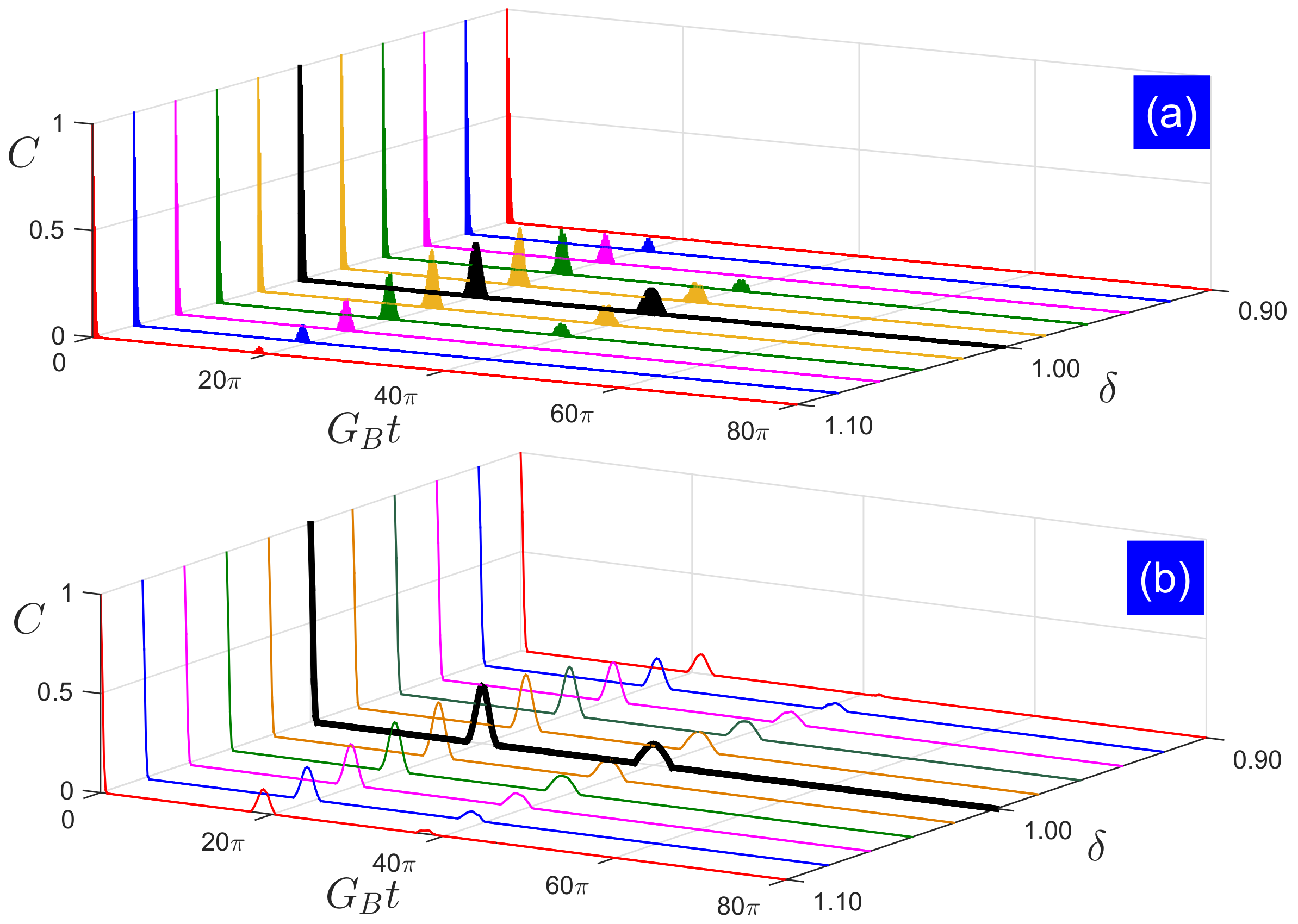
This concurrence evolution of two Jaynes–Cummings nodes reduces to that of two identical standard Jaynes–Cummings nodes at both the decay exponent and revival period. In Figure 3, we plot the long-time system dynamics under the coherent states with the large average photon number for analytical and numerical calculations. We find that the two-qubit entanglement exhibits sudden death phenomenon, and its peaks are not fully revived and decrease quadraticly as the gap between two qubit-field coupling strengths enlarges. The two-qubit entanglement decays exponentially as the evolution time increases. When , the revival period is linearly shifted to the “left” side, i.e., becoming shorter; while when , it is linearly shifted to the “right” side, i.e., becoming longer. Note that the numerical results in Figure 3b are not perfectly predicted by the analytical results in Figure 3a, and their main difference is the absence of Rabi-type oscillations during the revivals, i.e., the disappearance of tiny revivals in numerical results, which is not predicted by this analytical method [72]. Therefore, it is safe to say that the analytical results predict the numerical results for small gaps between two qubit-field coupling strengths in both the entanglement revival peek and period. Our result is physically important because the formula reveals analytically the relation between the entanglement evolution dynamics and two nonidentical qubit-field coupling strengths, which further clarifies the mechanism of entanglement sudden death and rebirth and provides another effective direction for entanglement control.
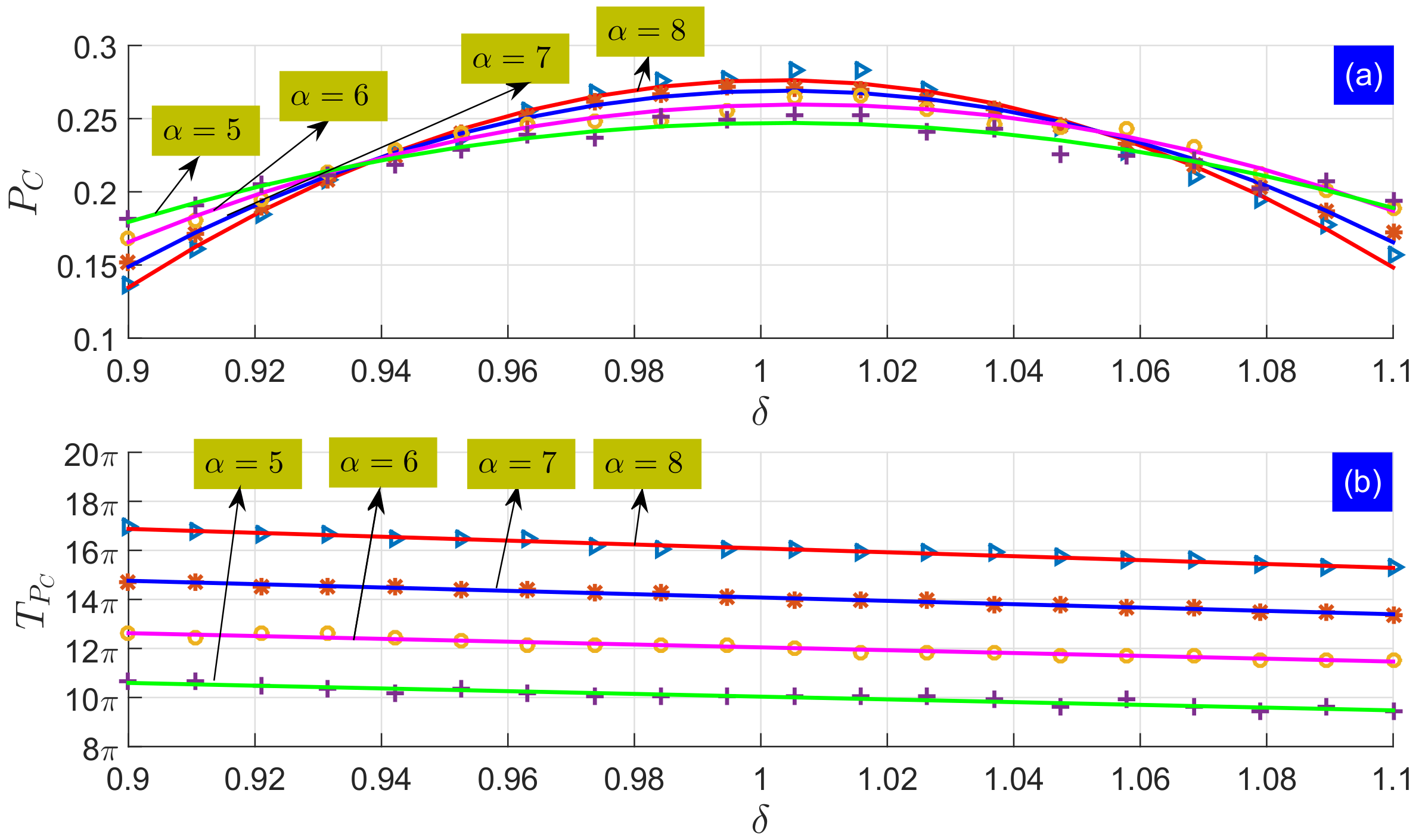
To quantitatively show the periodic modulations by the amplitude of coherent states and two qubit-field coupling strengths, we simulate the evolution dynamics with two other average photon numbers and for analytical and numerical results in Figure 4. We see that even when the average photon number decreases to 25, the analytical results can predict well the numerical results under small ratios . Figure 5 further shows that, for the same , peeks of the first revival envelope depend quadraticly on the ratio , and their periods linearly decrease as the ratio increases, which mathematically fits
This result demonstrates that the bigger gap between two qubit-field coupling strengths becomes, the smaller and faster entanglement revival will be, meaning that the increasing gap between two qubit-field coupling strengths accelerates the revival period and amplitude decay of two-qubit entanglement, which also can be explained from the decaying contribution of ratio factor within the exponents and within the cosine functions of Equation (38). Note that system asymmetry can be caused not only by the difference of the coupling strengths, but also by the difference of the amplitudes and . Based on numerical simulations, it is easy to find that the difference of the amplitudes and causes the similar influence on the two-qubit entanglement with that caused by the difference of the coupling strengths, i.e., the gap between two amplitudes affects both the period and amplitude of the entanglement revival. However, our method is hard to generalize to analytically give out the relation formula between this gap and entanglement, and this kind of interesting formula may be found elsewhere by a more effective method.
3. Conclusions
In conclusion, we have generalized the method of Ref. [72] to the model of two separate Jaynes–Cummings nodes, where the qubit-field coupling strength for each node is different. We use both the numerical and analytical methods to cases with vacuum-state and coherent-state fields, respectively. The numerical and analytical results have an excellent coincidence in the case of coherent-state fields for small gaps between two qubit-field coupling strengths. We find that the gap shifts the revival period and changes the revival amplitude of two-qubit entanglement. For vacuum-state fields, the maximal entanglement is fully revived after a gap-dependence period, within which the entanglement nonsmoothly decreases to zero and partly recovers without exhibiting a sudden death phenomenon. For strong coherent-state fields, the two-qubit entanglement decays exponentially as the evolution time increases, exhibiting sudden death phenomenon, and the increasing gap accelerates the revival period and amplitude decay of the entanglement. Our result finally demonstrates that when the average photon number is large enough, the decay exponent has a quadratic dependence on two qubit-field coupling strengths, and the non-full revival period is linearly shifted by the cooperative qubit-field coupling strength. Potential applications of our result, such as control of entanglement through changing the system parameters, are feasible in many simple experiments based on the fundamental Jaynes–Cummings Hamiltonian. In the future, we want to study further the large frequency detuning case and try to find a possible way to recover the full two-qubit entanglement under separate continuous-variable fields. Up to now, this model does not consider any dissipation, such as the cavity losses and atomic spontaneous emissions in extreme ultraviolet (XUV) and X-rays [75,76], which is an unavoidable decoherence problem and open question for keeping long-time entanglement in real experiments, and this kind of investigation could be done elsewhere by finding another effective method in the future.
Acknowledgments
This work is supported by the National Natural Science Foundation of China under Grant No. 11374054, the Natural Science Foundation of Fujian Province under Grant No. 2017J05005, and the fund from Fuzhou University under Nos. XRC-1566 and XRC-1639.
Author Contributions
All authors contributed equally to this article. The theoretical aspect of this work does not allow to point out any substantial authorship. All authors have read and approved the final manuscript.
Conflicts of Interest
The authors declare no conflict of interest.
References
- Nielsen, M.A.; Chuang, I.L. Quantum Computation and Quantum Information; Cambridge University Press: Cambridge, UK, 2000. [Google Scholar]
- Raimond, J.M.; Brune, M.; Haroche, S. Manipulating quantum entanglement with atoms and photons in a cavity. Rev. Mod. Phys. 2001, 73, 565–582. [Google Scholar] [CrossRef]
- Jaynes, E.T.; Cummings, F.W. Comparison of quantum and semiclassical radiation theories with application to the beam maser. Proc. IEEE 1963, 51, 89–109. [Google Scholar] [CrossRef]
- Zheng, S.B.; Guo, G.C. Efficient scheme for two-atom entanglement and quantum information processing in cavity QED. Phys. Rev. Lett. 2000, 85, 2392–2395. [Google Scholar] [CrossRef] [PubMed]
- Van Enk, S.J.; Cirac, J.I.; Zoller, P. Ideal quantum communication over noisy channels: A quantum optical implementation. Phys. Rev. Lett. 1997, 78, 4293–4296. [Google Scholar] [CrossRef]
- Ekert, A.K. Quantum cryptography based on Bell’s theorem. Phys. Rev. Lett. 1991, 67, 661–663. [Google Scholar] [CrossRef] [PubMed]
- Buluta, I.; Ashhab, S.; Nori, F. Natural and artificial atoms for quantum computation. Rep. Prog. Phys. 2011, 74, 104401. [Google Scholar] [CrossRef]
- Ashhab, S.; Niskanen, A.O.; Harrabi, K.; Nakamura, Y.; Picot, T.; de Groot, P.C.; Harmans, C.J.P.M.; Mooij, J.E.; Nori, F. Interqubit coupling mediated by a high-excitation-energy quantum object. Phys. Rev. B 2008, 77, 014510. [Google Scholar] [CrossRef]
- Rivas, A.; Huelga, S.F.; Plenio, M.B. Quantum non-Markovianity: Characterization, quantification and detection. Rep. Prog. Phys. 2014, 77, 094001. [Google Scholar] [CrossRef] [PubMed]
- Mortezapour, A.; Borji, M.A.; lo Franco, R. Protecting entanglement by adjusting the velocities of moving qubits inside non-Markovian environments. Laser Phys. Lett. 2017, 14, 055201. [Google Scholar] [CrossRef]
- Mortezapour, A.; Borji, M.A.; lo Franco, R. Non-Markovianity and coherence of a moving qubit inside a leaky cavity. arXiv, 2017; arXiv:1705.00887. [Google Scholar]
- Lo Franco, R.; d’Arrigo, A.; Falci, G.; Compagno, G.; Paladino, E. Spin-echo entanglement protection from random telegraph noise. Phys. Scr. 2013, 153, 014043. [Google Scholar] [CrossRef]
- Aolita, L.; de Melo, F.; Davidovich, L. Open-system dynamics of entanglement: A key issues review. Rep. Prog. Phys. 2015, 78, 042001. [Google Scholar] [CrossRef] [PubMed]
- Lo Franco, R.; Bellomo, B.; Maniscalco, S.; Compagno, G. Dynamics of quantum correlations in two-qubit systems within non-Markovian environments. Int. J. Mod. Phys. B 2013, 27, 1345053. [Google Scholar] [CrossRef]
- De Vega, I.; Alonso, D. Dynamics of non-Markovian open quantum systems. Rev. Mod. Phys. 2017, 89, 015001. [Google Scholar] [CrossRef]
- Lo Franco, R.; Compagno, G. Overview on the phenomenon of two-qubit entanglement revivals in classical environments. arXiv, 2016; arXiv:1608.05970. [Google Scholar]
- D’Arrigo, A.; lo Franco, R.; Benenti, G.; Paladino, E.; Falci, G. Recovering entanglement by local operations. Ann. Phys. 2014, 350, 211–224. [Google Scholar] [CrossRef]
- Leggio, B.; lo Franco, R.; Soares-Pinto, D.O.; Horodecki, P.; Compagno, G. Distributed correlations and information flows within a hybrid multipartite quantum-classical system. Phys. Rev. A 2015, 92, 032311. [Google Scholar] [CrossRef]
- González-Gutiérrez, C.A.; Román-Ancheyta, R.; Espitia, D.; lo Franco, R. Relations between entanglement and purity in non-Markovian dynamics. Int. J. Quantum Inform. 2016, 14, 1650031. [Google Scholar] [CrossRef]
- Sciara, S.; lo Franco, R.; Compagno, G. Universality of Schmidt decomposition and particle identity. Sci. Rep. 2017, 7, 44675. [Google Scholar] [CrossRef] [PubMed]
- Bellomo, B.; lo Franco, R.; Compagno, G. N identical particles and one particle to entangle them all. arXiv, 2017; arXiv:1704.06359. [Google Scholar]
- Lo Franco, R.; d’Arrigo, A.; Falci, G.; Compagno, G.; Paladino, E. Preserving entanglement and nonlocality in solid-state qubits by dynamical decoupling. Phys. Rev. B 2014, 90, 054304. [Google Scholar] [CrossRef]
- D’Arrigo, A.; Benenti, G.; lo Franco, R.; Falci, G.; Paladino, E. Hidden entanglement, system-environment information flow and non-Markovianity. Int. J. Quantum Inform. 2014, 12, 1461005. [Google Scholar] [CrossRef]
- Trapani, J.; Bina, M.; Maniscalco, S.; Paris, M.G. Collapse and revival of quantum coherence for a harmonic oscillator interacting with a classical fluctuating environment. Phys. Rev. A 2015, 91, 022113. [Google Scholar] [CrossRef]
- D’Arrigo, A.; lo Franco, R.; Benenti, G.; Paladino, E.; Falci, G. Hidden entanglement in the presence of random telegraph dephasing noise. Phys. Scr. 2013, 153, 014014. [Google Scholar] [CrossRef]
- Lo Franco, R.; d’Arrigo, A.; Falci, G.; Compagno, G.; Paladino, E. Entanglement dynamics in superconducting qubits affected by local bistable impurities. Phys. Scr. 2012, 147, 014019. [Google Scholar] [CrossRef]
- Bellomo, B.; Compagno, G.; lo Franco, R.; Ridolfo, A.; Savasta, S. Entanglement dynamics of two independent cavity-embedded quantum dots. Phys. Scr. 2011, 143, 014004. [Google Scholar] [CrossRef]
- Dijkstra, A.G.; Tanimura, Y. Non-Markovian entanglement dynamics in the presence of system-bath coherence. Phys. Rev. Lett. 2010, 104, 250401. [Google Scholar] [CrossRef] [PubMed]
- Lo Franco, R.; Compagno, G. Quantum entanglement of identical particles by standard information-theoretic notions. Sci. Rep. 2016, 6, 20603. [Google Scholar] [CrossRef] [PubMed]
- Bellomo, B.; lo Franco, R.; Andersson, E.; Cresser, J.D.; Compagno, G. Dynamics of correlations due to a phase-noisy laser. Sci. Rep. 2012, 147, 014004. [Google Scholar] [CrossRef]
- Maniscalco, S.; Francica, F.; Zaffino, R.L.; Gullo, N.L.; Plastina, F. Protecting entanglement via the quantum Zeno effect. Phys. Rev. Lett. 2008, 100, 090503. [Google Scholar] [CrossRef] [PubMed]
- Bellomo, B.; lo Franco, R.; Maniscalco, S.; Compagno, G. Two-qubit entanglement dynamics for two different non-Markovian environments. Phys. Scr. 2010, T140, 014014. [Google Scholar] [CrossRef]
- Bellomo, B.; Compagno, G.; lo Franco, R.; Ridolfo, A.; Savasta, S. Dynamics and extraction of quantum discord in a multipartite open system. Int. J. Quantum Inform. 2011, 9, 1665–1676. [Google Scholar] [CrossRef]
- Lo Franco, R. Nonlocality threshold for entanglement under general dephasing evolutions: A case study. Quantum Inform. Process. 2016, 15, 2393–2404. [Google Scholar] [CrossRef]
- Silva, I.A.; Souza, A.M.; Bromley, T.R.; Cianciaruso, M.; Marx, R.; Sarthour, R.S.; Oliveira, I.S.; lo Franco, R.; Glaser, S.J.; Deazevedo, E.R.; et al. Observation of time-invariant coherence in a nuclear magnetic resonance quantum simulator. Phys. Rev. Lett. 2016, 117, 160402. [Google Scholar] [CrossRef] [PubMed]
- Orieux, A.; D’Arrigo, A.; Ferranti, G.; lo Franco, R.; Benenti, G.; Paladino, E.; Falci, G.; Sciarrino, F.; Mataloni, P. Experimental on-demand recovery of entanglement by local operations within non-Markovian dynamics. Sci. Rep. 2015, 5, 8575. [Google Scholar] [CrossRef] [PubMed]
- Man, Z.X.; Xia, Y.J.; lo Franco, R. Cavity-based architecture to preserve quantum coherence and entanglement. Sci. Rep. 2015, 5, 13843. [Google Scholar] [CrossRef] [PubMed]
- Rendell, R.W.; Rajagopal, A.K. Revivals and entanglement from initially entangled mixed states of a damped Jaynes–Cummings model. Phys. Rev. A 2003, 67, 062110. [Google Scholar] [CrossRef]
- Rempe, G.; Walther, H.; Klein, N. Observation of quantum collapse and revival in a one-atom maser. Phys. Rev. Lett. 1987, 58, 353–356. [Google Scholar] [CrossRef] [PubMed]
- Brune, M.; Schmidt-Kaler, F.; Maali, A.; Dreyer, J.; Hagley, E.; Raimond, J.M.; Haroche, S. Quantum Rabi oscillation: A direct test of field quantization in a cavity. Phys. Rev. Lett. 1996, 76, 1800–1803. [Google Scholar] [CrossRef] [PubMed]
- Meekhof, D.M.; Monroe, C.; King, B.E.; Itano, W.M.; Wineland, D.J. Generation of nonclassical motional states of a trapped atom. Phys. Rev. Lett. 1996, 76, 1796–1799. [Google Scholar] [CrossRef] [PubMed]
- Boca, A.; Miller, R.; Birnbaum, K.M.; Boozer, A.D.; McKeever, J.; Kimble, H.J. Observation of the vacuum Rabi spectrum for one trapped atom. Phys. Rev. Lett. 2004, 93, 233603. [Google Scholar] [CrossRef] [PubMed]
- Gea-Banacloche, J. Collapse and revival of the state vector in the Jaynes–Cummings model: An example of state preparation by a quantum apparatus. Phys. Rev. Lett. 1990, 65, 3385–3388. [Google Scholar] [CrossRef] [PubMed]
- Phoenix, S.J.D.; Knight, P.L. Establishment of an entangled atom-field state in the Jaynes–Cummings model. Phys. Rev. A 1991, 44, 6023–6029. [Google Scholar] [CrossRef] [PubMed]
- Sainz, I.; Björk, G. Quantum error correction may delay, but also cause, entanglement sudden death. Phys. Rev. A 2008, 77, 052307. [Google Scholar] [CrossRef]
- Chan, S.; Reid, M.D.; Ficek, Z. Entanglement evolution of two remote and non-identical Jaynes–Cummings atoms. J. Phys. B 2009, 42, 065507. [Google Scholar] [CrossRef]
- Agarwal, G.S. Vacuum-field Rabi splittings in microwave absorption by Rydberg atoms in a cavity. Phys. Rev. Lett. 1984, 53, 1732–1734. [Google Scholar] [CrossRef]
- Shen, L.T.; Chen, R.X.; Wu, H.Z.; Yang, Z.B. Distributed manipulation of two-qubit entanglement with coupled continuous variables. J. Opt. Soc. Am. B 2015, 32, 297–302. [Google Scholar] [CrossRef]
- Yu, T.; Eberly, J.H. Sudden death of entanglement. Science 2009, 323, 598–601. [Google Scholar] [CrossRef] [PubMed]
- Kraus, B.; Cirac, J.I. Discrete entanglement distribution with squeezed light. Phys. Rev. Lett. 2004, 92, 013602. [Google Scholar] [CrossRef] [PubMed]
- Sornborger, A.T.; Cleland, A.N.; Geller, M.R. Superconducting phase qubit coupled to a nanomechanical resonator: Beyond the rotating-wave approximation. Phys. Rev. A 2004, 70, 052315. [Google Scholar] [CrossRef]
- Paternostro, M.; Son, W.; Kim, M.S.; Falci, G.; Palma, G.M. Dynamical entanglement transfer for quantum-information networks. Phys. Rev. A 2004, 70, 022320. [Google Scholar] [CrossRef]
- Paternostro, M.; Son, W.; Kim, M.S. Complete conditions for entanglement transfer. Phys. Rev. Lett. 2004, 92, 197901. [Google Scholar] [CrossRef] [PubMed]
- Zhou, L.; Yang, G.H. Entanglement reciprocation between atomic qubits and an entangled coherent state. J. Phys. B 2006, 39, 5143–5150. [Google Scholar] [CrossRef]
- Hu, Y.H.; Tan, Y.G. Delaying disappearance of entanglement by the linear modulation of atom-field coupling. Phys. Scr. 2014, 89, 075103. [Google Scholar] [CrossRef]
- Xu, J.S.; Li, C.F.; Gong, M.; Zou, X.B.; Shi, C.H.; Chen, G.; Guo, G.C. Experimental demonstration of photonic entanglement collapse and revival. Phys. Rev. Lett. 2010, 104, 100502. [Google Scholar] [CrossRef] [PubMed]
- Eleuch, H.; Bennaceur, R. An optical soliton pair among absorbing three-level atoms. J. Opt. A 2003, 5, 528–533. [Google Scholar] [CrossRef]
- Eleuch, H. Autocorrelation function of microcavity-emitting field in the linear regime. Eur. Phys. J. D 2008, 48, 139–143. [Google Scholar] [CrossRef]
- Eleuch, H. Entanglement and autocorrelation function in semiconductor microcavities. Int. J. Mod. Phys. B 2010, 24, 5653–5662. [Google Scholar] [CrossRef]
- Sete, E.A.; Eleuch, H.; Ooi, C.R. Light-to-matter entanglement transfer in optomechanics. J. Opt. Soc. Am. B 2014, 31, 2821–2828. [Google Scholar] [CrossRef]
- Rafsanjani, S.M.H.; Eberly, J.H. Coherent control of multipartite entanglement. Phys. Rev. A 2015, 91, 012313. [Google Scholar] [CrossRef]
- Lawrence, J. Mermin inequalities for perfect correlations in many-qutrit systems. Phys. Rev. A 2017, 95, 042123. [Google Scholar] [CrossRef]
- Scully, M.O.; Zubairy, M.S. Quantum Optics; Cambridge University Press: Cambridge, UK, 1997. [Google Scholar]
- Braunstein, S.L.; van Loock, P. Quantum information with continuous variables. Rev. Mod. Phys. 2005, 77, 513–577. [Google Scholar] [CrossRef]
- Adesso, G.; Illuminati, F. Entanglement in continuous-variable systems: Recent advances and current perspectives. J. Phys. A 2007, 40, 7821–7880. [Google Scholar] [CrossRef]
- Casagrande, F.; Lulli, A.; Paris, M.G. Improving the entanglement transfer from continuous-variable systems to localized qubits using non-Gaussian states. Phys. Rev. A 2007, 75, 032336. [Google Scholar] [CrossRef]
- Blanco, P.; Mundarain, D. Faithful entanglement transference from qubits to continuous variable systems. J. Phys. B 2011, 44, 105501. [Google Scholar] [CrossRef]
- Ballester, D. Entanglement accumulation, retrieval, and concentration in cavity QED. Phys. Rev. A 2009, 79, 062317. [Google Scholar] [CrossRef]
- Lee, J.; Paternostro, M.; Kim, M.S.; Bose, S. Entanglement reciprocation between qubits and continuous variables. Phys. Rev. Lett. 2006, 96, 080501. [Google Scholar] [CrossRef] [PubMed]
- Paternostro, M.; Kim, M.S.; Palma, G.M. Accumulation of entanglement in a continuous variable memory. Phys. Rev. Lett. 2007, 98, 140504. [Google Scholar] [CrossRef] [PubMed]
- Yönaç, M.; Eberly, J.H. Qubit entanglement driven by remote optical fields. Opt. Lett. 2008, 33, 270–272. [Google Scholar] [CrossRef] [PubMed]
- Yönaç, M.; Eberly, J.H. Coherent-state control of noninteracting quantum entanglement. Phys. Rev. A 2010, 82, 022321. [Google Scholar] [CrossRef]
- Wootters, W.K. Entanglement of formation of an arbitrary state of two qubits. Phys. Rev. Lett. 1998, 80, 2245. [Google Scholar] [CrossRef]
- Yu, T.; Eberly, J.H. Evolution from entanglement to decoherence of bipartite mixed X states. Quantum Inf. Comput. 2007, 7, 459–468. [Google Scholar]
- Sete, E.A.; Svidzinsky, A.A.; Eleuch, H.; Yang, Z.; Nevels, R.D.; Scully, M.O. Correlated spontaneous emission on the Danube. J. Mod. Opt. 2010, 57, 1311–1330. [Google Scholar] [CrossRef]
- Sete, E.A.; Svidzinsky, A.A.; Rostovtsev, Y.V.; Eleuch, H.; Jha, P.K.; Suckewer, S.; Scully, M.O. Using Quantum Coherence to Generate Gain in the XUV and X-ray: Gain-Swept Superradiance and Lasing without Inversion. IEEE J. Sel. Top. Quantum Electron. 2012, 18, 541–553. [Google Scholar] [CrossRef]
Figure 1.
Sketch illustrating two separate Jaynes–Cummings nodes. Qubits A and B are independently placed in Nodes 1 and 2, resonantly coupling to the fields a and b, respectively. There is not any interaction between A and B or between a and b.
Figure 1.
Sketch illustrating two separate Jaynes–Cummings nodes. Qubits A and B are independently placed in Nodes 1 and 2, resonantly coupling to the fields a and b, respectively. There is not any interaction between A and B or between a and b.
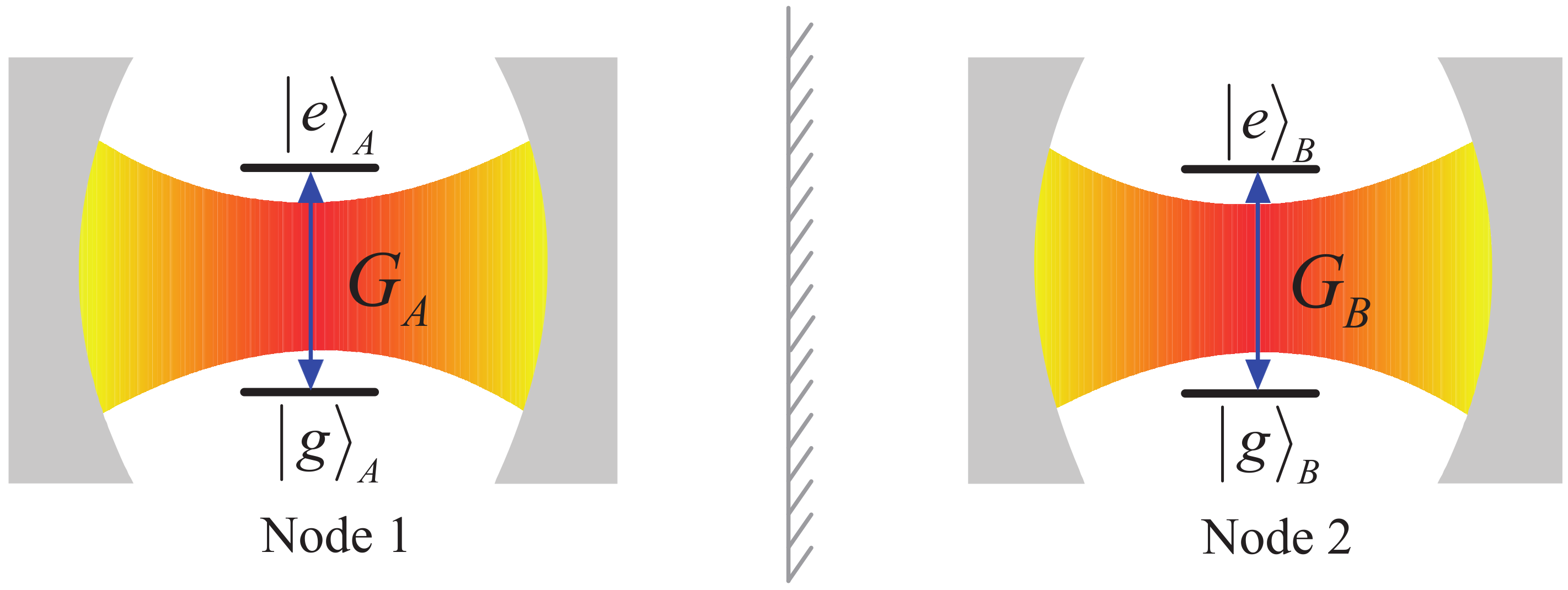
Figure 2.
Time-dependent evolution of C for: (a) ; (b) ; and (c) . The corresponding periods are , , and , respectively.
Figure 2.
Time-dependent evolution of C for: (a) ; (b) ; and (c) . The corresponding periods are , , and , respectively.
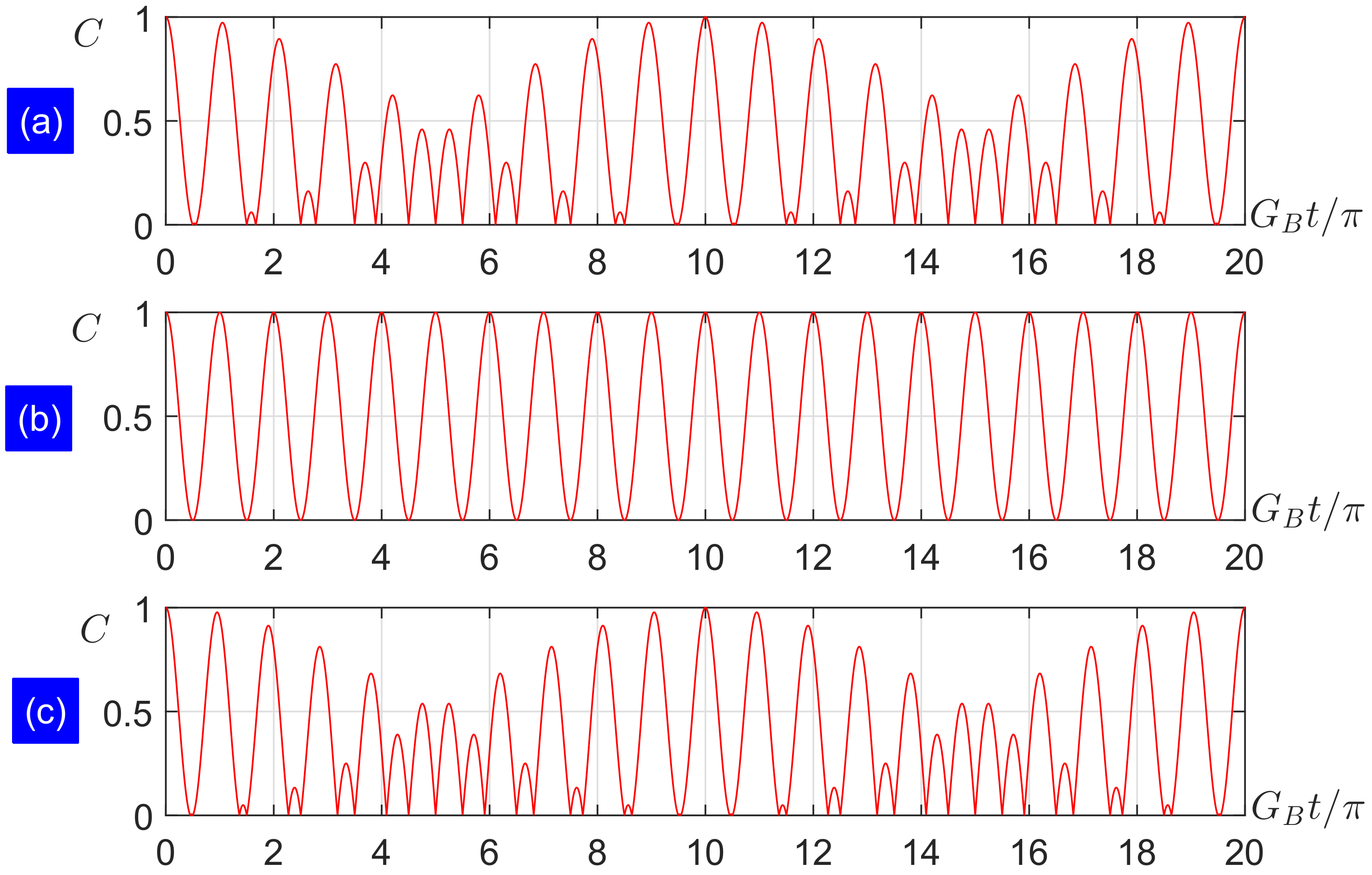
Figure 3.
Two-qubit concurrence as a function of the evolution time under different ratios with : (a) analytical results and (b) numerical results, where analytical results are based on the X-form in Equation (15) and numerical results are based on the original .
Figure 3.
Two-qubit concurrence as a function of the evolution time under different ratios with : (a) analytical results and (b) numerical results, where analytical results are based on the X-form in Equation (15) and numerical results are based on the original .

Figure 4.
Two-qubit concurrence evolves with time under different ratios for analytical results ((a) and (b) ) and numerical results ((c) and (d) ).
Figure 4.
Two-qubit concurrence evolves with time under different ratios for analytical results ((a) and (b) ) and numerical results ((c) and (d) ).
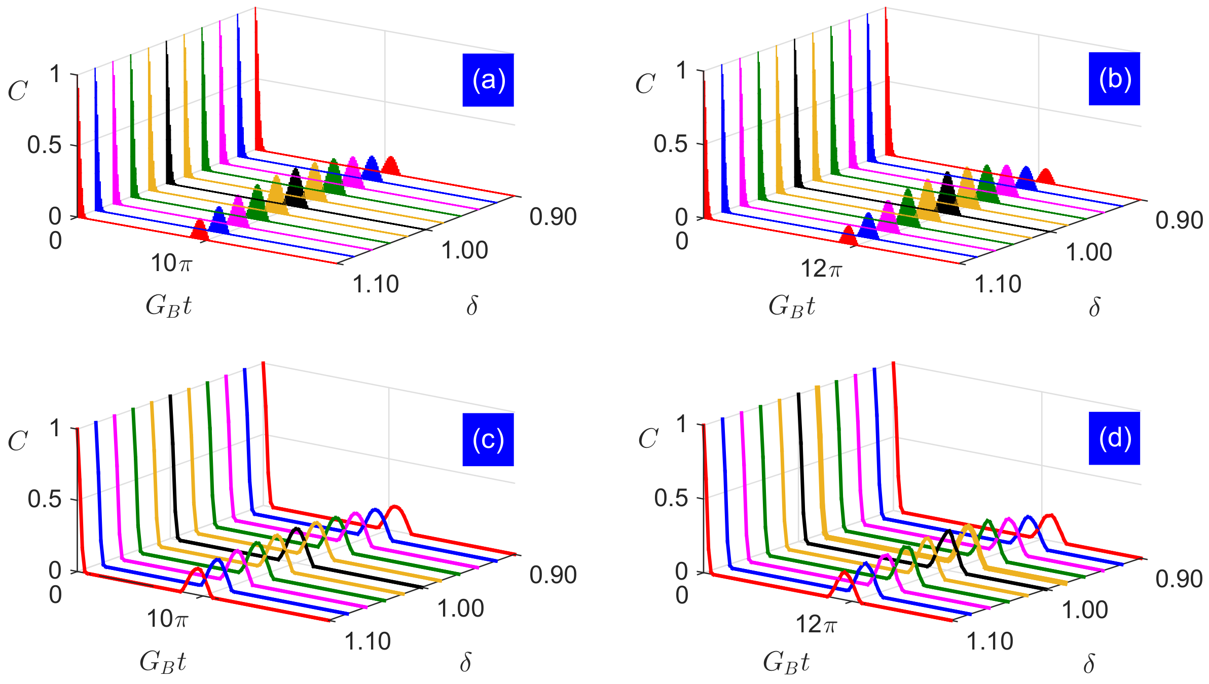
Figure 5.
Characteristics of the first revival envelope versus the ratio for different : (a) peek and (b) period .
Figure 5.
Characteristics of the first revival envelope versus the ratio for different : (a) peek and (b) period .

© 2017 by the authors. Licensee MDPI, Basel, Switzerland. This article is an open access article distributed under the terms and conditions of the Creative Commons Attribution (CC BY) license (http://creativecommons.org/licenses/by/4.0/).
Share and Cite
MDPI and ACS Style
Shen, L.-T.; Shi, Z.-C.; Wu, H.-Z.; Yang, Z.-B. Dynamics of Entanglement in Jaynes–Cummings Nodes with Nonidentical Qubit-Field Coupling Strengths. Entropy 2017, 19, 331. https://doi.org/10.3390/e19070331
AMA Style
Shen L-T, Shi Z-C, Wu H-Z, Yang Z-B. Dynamics of Entanglement in Jaynes–Cummings Nodes with Nonidentical Qubit-Field Coupling Strengths. Entropy. 2017; 19(7):331. https://doi.org/10.3390/e19070331
Chicago/Turabian StyleShen, Li-Tuo, Zhi-Cheng Shi, Huai-Zhi Wu, and Zhen-Biao Yang. 2017. "Dynamics of Entanglement in Jaynes–Cummings Nodes with Nonidentical Qubit-Field Coupling Strengths" Entropy 19, no. 7: 331. https://doi.org/10.3390/e19070331
Note that from the first issue of 2016, this journal uses article numbers instead of page numbers. See further details here.