Information Entropy in Predicting Location of Observation Points for Long Tunnel

Department of Hydraulic and Hydropower Engineering, Tsinghua University, Beijing 100084, China
*
Authors to whom correspondence should be addressed.
Entropy 2017, 19(7), 332; https://doi.org/10.3390/e19070332
Submission received: 3 May 2017
/
Revised: 24 June 2017
/
Accepted: 29 June 2017
/
Published: 4 July 2017
Abstract
:Based on the Markov model and the basic theory of information entropy, this paper puts forward a new method for optimizing the location of observation points in order to obtain more information from limited geological investigation. According to the existing data from observation points data, classification of tunnel geological lithology was performed, and various lithology distribution were determined along the tunnel using the Markov model and theory. On the basis of the information entropy theory, the distribution of information entropy was obtained along the axis of the tunnel. Therefore, different information entropy could be acquired by calculating different classification of rocks. Furthermore, uncertainty increases when information entropy increased. The maximum entropy indicates maximum uncertainty and thus, this value determines the position of the new drilling hole. A new geology situation will be decided by the maximum entropy for the lowest accuracy. Optimal distribution will be obtained after recalculating, using the new location of the geology situation. Taking the engineering for the Bashiyi Daban water diversion tunneling in Xinjiang as a case, the maximum information entropy of the geological conditions was analyzed by the method proposed in the present study, with 25 newly added geology observation points along the axis of the 30-km tunnel. The results proved the validity of the present method. The method and results in this paper may be used not only to predict the geological conditions of underground engineering based on the investigated geological information, but also to optimize the distribution of the geology observation points.
1. Introduction
Engineering geological investigation provides the basic information through the process of conducting a feasibility study, in addition to design and construction, when building a long tunnel. In fact, the number of investigation points could significantly contribute to determining the cost of a tunnel project [1]. As shown in Figure 1 [1], as the number of investigation points increases, there will be a richer amount of geological data obtained, a lower total project cost and lower construction cost. However, there is a plateau with this increase, as the details of the geological data do not increase to a significant extent after the number of investigation points reaches a certain value. At the same time, the construction cost remains unchanged, and the investigation cost is directly proportional to the number of investigation points, so the total project cost will increase rather than decrease.
The value of the minimum total cost of a project corresponds to the optimal number of observation points. Due to many influence factors affecting the cost, this present study did not set the total project cost as the optimization goal, but focused on optimizing the locations of new geological investigation sites. In order to obtain more geological information under the condition of less investigation points, this paper puts forward a new optimization method for geological investigation points based on the Markov model and the basic theory of information entropy.
Each single geological parameter is regarded as a discrete-state continuous-space Markov process in the Markov model [2,3,4,5]. Based on the current status of the system, the Markov approach can predict the future development trend and state of the system by establishing a transfer matrix [6,7]. It is widely used in the field of science and technology [8,9,10,11]. The Markov model has been used in simulations of stochastic reservoir lithofacies [12]. In addition, this approach has played an important role in simulation analysis of TBM construction [13,14].
Based on the second law of thermodynamics, the concept of entropy is a function of the state that describes an irreversible process. Shannon [15] first cited the entropy concept in information theory and defined it as information entropy, which indicates the average information content that occurs without redundancy. The information entropy is equal to the expected number of bits needed to identify which micro-state it is in, given the macro-state [16]. The information entropy has been used in the canonical genetic code [17]. Furthermore, the information entropy is regarded as the measurement of the relationship between nodes including direct and indirect neighbors [18].
In order to optimize the location of observation points, the information entropy based on the Markov model is introduced to calculate the geological uncertainty when predicting geological conditions along the tunnel. This method was selected for its rigorous mathematical logic, as well as the convenience for engineering practice. Section 2 presents the methodology of the geologic prediction based on Markov model and the information entropy approach comprehensively. The study in Section 3 aims to examine its application for the Bashiyi Daban water diversion tunnel project carefully. Furthermore, Section 4 offers some improvements and conclusions.
2. Methodology
2.1. Probabilistic Estimation of Geologic Parameters along the Tunnel
The characteristics of the Markov model stipulate that the future state of the system is not connected with the previous state, but is determined by the current state [19]. The formation of the geological stratum will obey the basic physical and chemical laws, despite numerous other random influences. For instance, many geological processes are related to the Markov properties, such as occurrence stratum, stratigraphic accumulation, sedimentary diffusion and magnetic activity [20]. Therefore, the Markov model can be applied to changes in lithology. This paper adopts the geologic prediction model created by Ioannou [3]. The Markov model implementation process is as follows:
Step 1: Estimate the transition probability (Pij) from the state i to the state j, in addition to the transition intensity coefficient (ξi) of the state i, using statistical procedures through the following equation:
where Hi represents the length for which geologic parameter remains within a particular state i; and E(Hi) is the expected length that is occupied by the state i of the geologic parameter.
Step 2: Calculate the transition intensity matrix A through the transition intensity coefficient and probability according to the following equation:
Step 3: Calculate the interval transition probability matrix W (S0, S) according to the following equation:
where wij (S0, S) is the probability of the geological parameter that the state will be j at the location S, given the state is i at the reference location S0. The interval transition probability is solved based on the expansion of the general solution of the Kolmogorov's differential equation [21,22].
Step 4: Calculate the state probability X(S) at the location S using the state probability X(S0) of the geologic parameter at the certain location S0.
Step 5: Calculate the posterior probabilities at the observation location according to the data from the observation points.
where l denotes the rock type; t denotes the rock types that are classified by the geological investigation code [23]; Sm denotes the observational location along the tunnel; m represents the mth observation site; and Y(Sm) denotes the rock type at the mth observation site. denotes the posterior probability matrix at the mth observation site.
Step 6: Update the posterior interval transition probabilities according to the data from the investigation points and the Bayesian technique as shown in Equation (8):
where Sd denotes the last observational location along the tunnel; and d represents the last observation site.
Step 7: Determine the final updated probability of the geologic parameters at location S through Equation (9):
where Xi(S0) denotes the probability of the geologic parameter being i at the location of a tunnel entrance; and Xj(S) denotes the probability being j at the location S.
As presented above, using the posterior probabilities at the observation location and all the desired parameter states, it is possible to obtain the rock types along the tunnel alignment. The purpose of the Markov model for geologic predictions is the formation of a ground class profile so that it would be used to calculate the geological uncertainty along the tunnel alignment.
2.2. Location Optimization of Geological Investigation Points
The priority aim of optimizing the locations of observation points is to acquire more information with fewer tunnel geological investigation points. The interval information entropy can be used to measure the information uncertainty of various locations along the tunnel alignment, while the location of the maximum information entropy corresponds to the optimal location of new geological investigation points. The different stages of locational optimization can be expressed as follows:
Stage 1: Calculation of the probability Xj(S) of the geologic parameters at various locations along the tunnel alignment based on the above Markov geologic prediction approach:
where Xj(S) denotes the probability being j at the location S; and t denotes rock types that are classified by the geological investigation code [23].
Stage 2: Calculation of the length interval information entropy at various locations according to the following equation [15]:
Furthermore, , which means the interval information entropy at the observational location is 0.
Stage 3: Calculation of the total information entropy ES for the tunnel. The total information entropy is used to measure the information uncertainty of the tunnel:
where Sstart denotes the starting point; and Send denotes the end point of the tunnel. As there is no definite mathematical expression related to H(S) in practical applications, we were unable to obtain the total information entropy through mathematical integration. In this present study, the trapezoidal method was used to calculate the total information entropy ES.
Stage 4: Construction of the optimization model for adding exploration points:
where Sbi denotes the new exploration point. According to the equation , the following equations can be obtained:
Stage 5: Solution of the optimization model. The function of H(S) is a convex function, while the interval probabilities at the locations between Sm and Sm+1 are only determined by the geologic parameters at Sm and Sm+1. Therefore, the optimization model can be updated as the following:
where d denotes the total number of observation sites.
Stage 6: Determination of the other optimal locations. Based on the above processes, the probability Y(Sb1) would be complemented at the new investigation location Sb1. Therefore, the probability of the geologic parameters at various locations along the tunnel alignment would be updated. Following this, the next optimal location Sb2 can be determined using the same method. In the range of the permitted numbers, the other optimal locations of geological investigation would be determined in the same manner.
3. Case Study
The newly proposed method for optimizing the locations of the geological investigation points was applied to the engineering of the Bashiyi Daban water diversion tunneling in Xinjiang province to demonstrate its validity. The length of the water diversion tunnel is 30,691 m, while the rock properties are categorized into II, III1, III2, IV and V types, according to the geological investigation code in China [23].
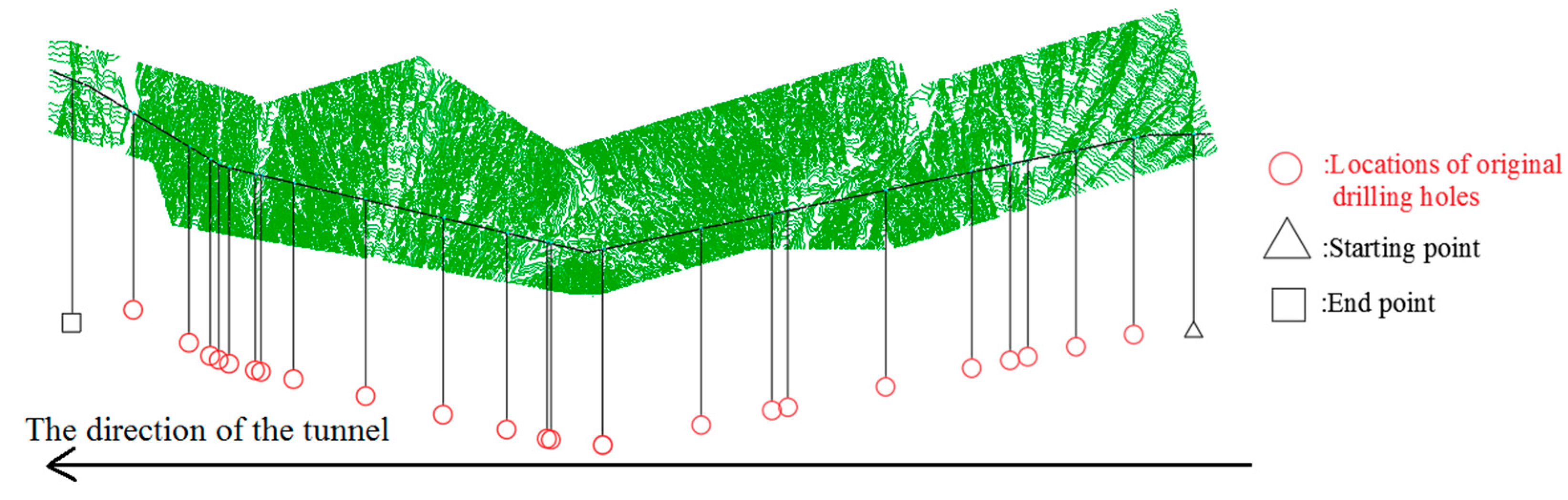
There are 25 boring observation points, including the starting point and the end point along the tunnel alignment. The distribution of various observation sites is illustrated in Figure 2. The locations and rock types of 25 observations are presented in Table 1.
Regardless of measurement error, it is considered that the probability of the boring observation points is 1. For example, the fifth observation point is located 4841 m away from the tunnel entrance, with the surrounding rock being the fourth (IV) type through geological examination. Thus, the following equation is satisfied:
where 1–5 represent the II, III1, III2, IV and V types of surrounding rock, respectively.
The explored geologic information would be used to update the posterior interval transition probabilities according to the Bayesian technique. The transition probability matrix P for all types of surrounding rock was determined by Equation (1) to be as follows:
According to Equation (2), mentioned previously, the transition intensity coefficients of all the types of surrounding rocks were calculated to be: ξ1 = 0.00218, ξ2 = 0.000349, ξ3 = 0.000791, ξ4 = 0.000788 and ξ5 = 0.000351. The transition intensity matrix A was calculated through Equation (3) to be as follows:
Based on the 25 observation points, the probabilistic rock type along the tunnel alignment was determined using Equation (9), as shown in Figure 3.
Three points are selected for the prediction of positions of other points to calculate the information entropy. These points were the starting point Sstart, the end point Send and the mid-point of Bashiyi Daban tunnel. Following this, the information entropy was calculated by real observation points. Therefore, the advantage of the optimal method would be illustrated by comparing the two information entropies obtained.
Step 1: Calculating the length interval information entropy at various locations. The information entropy distribution according to the original 25 observation points is shown in Figure 4. As the total information entropy ES is a definite integration, we used numerical integration to calculate it, setting the integration step to 1 for simplicity. The total information entropy Es can be calculated based on Equation (13), which was found to be 12,773, according to this method.
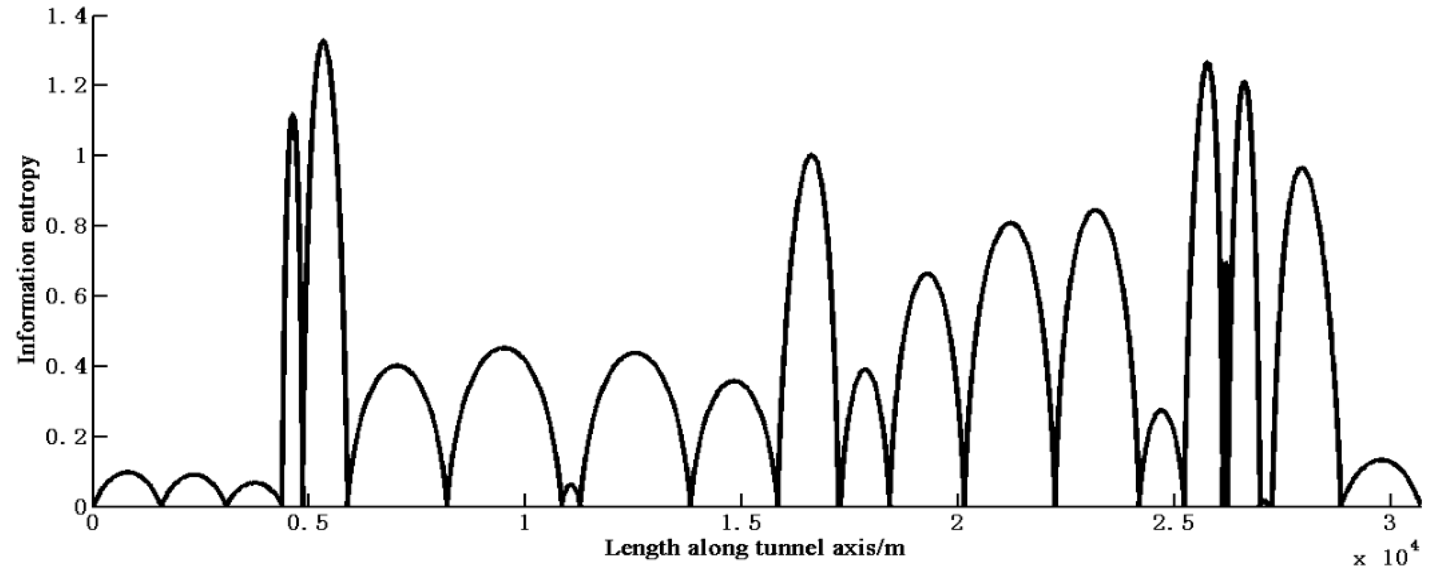
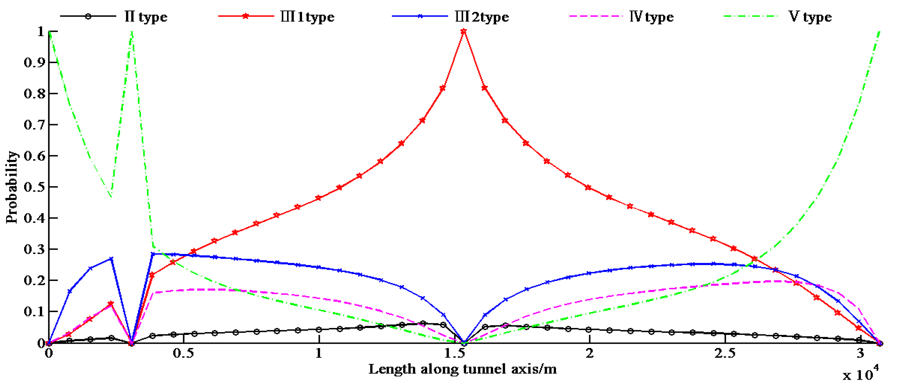
Step 2: Calculating the probabilistic rock type along the tunnel alignment and the interval information entropy at various locations (1 m as a unit) based on the three existing observations. Figure 5 shows the probability distribution of rock types. The information entropy distribution is also shown in Figure 6, while the total information entropy Es is 37,129 according to Equation (15) (on the condition of Si = 1, for simplicity) at that time.
where the arrow position Sb1 is the optimal location and it is also the new geological investigation location.
Step 3: Calculating the probabilistic rock type and the interval information entropy based on the new optimal location. As the engineering for the Bashiyi Daban water diversion tunneling has been completed, the rock types along the tunnel alignment have been revealed. Therefore, the rock type of the new observation points is type IV.
Figure 7 shows the updated distribution of probability based on the 4 observations. The updated information entropy distribution and the next optimal location are shown in Figure 8, with the total information entropy Es being 35,172 at that time.
Step 4: Determine the other optimal locations according to the same process. Table 2 includes the quantities, locations, the calculated rock types and the information entropy of the new additional observation sites.
Table 2 shows that the total information entropy is 8489, based on the optimal method of investigation site location, which is far lower than the value obtained in the original method. Furthermore, using only 16 geological observations in accordance with the optimal method achieves the same level of certainty as using 25 observation sites with the original method. Therefore, the proposed method for positioning of exploration points can achieve the goal of reducing the number of observation points. The updated distribution of probability and information entropy are shown in Figure 9 and Figure 10.
4. Discussion
The Markov model for geologic predictions is a good complement for geophysical prospecting, because it can predict the surrounding rock type in a probabilistic way. Based on the provided probabilities of the surrounding rock types, information entropy can be used to evaluate the uncertainty along the tunnel alignment.
In order to compare the results of the actual geology, the encountered geological profile is illustrated in Figure 9. It shows that the predicted rock type is fairly consistent with the actual rock type. Therefore, the Markov model was able to be used to predict the rock type, and the optimized method of the geological investigation points is validated.
Figure 11 shows the relationship between the number of investigation points and total information entropy. As shown in Figure 11, there will be less information entropy with an increase in the number of investigation points. Furthermore, using only 16 geological investigation observations for the optimal method can achieve the same requirement as the original 25 observation sites. In essence, using the optimized 16 geological observation points can obtain the same information obtained by the 25 observation points without optimization. In order to highlight the improvement in the proposed method for positioning of the exploration points, we compared the total information entropy of equidistant distributions. We calculated the total information entropy of 14–25 observation points, which have an equidistant distribution along the tunnel. As shown in Figure 11, for the equidistant distribution method, the values of the total information entropy do not all decrease with an increase in the number of investigation points. Furthermore, the total information entropy of the equidistant distribution method is higher than our proposed method with the same number of observation points.
Apart from the merits presented above, this new optimization method has some flaws and shortcomings. Essentially, in the probabilistic assessment of Markovian geophysical prospecting, more empirical data are needed to ensure the accuracy of the estimation. Expert judgments are reliable for the evaluation of mean values, but not for assessing the variances [24].
5. Conclusions
In this study, a new optimization method for the positioning of geological investigation points based on the Markov model and the basic theory of information entropy was proposed. The additional locations based on the new optimization method are able to obtain more information than the original method, so total information entropy would decrease.
The case study of the engineering for the Bashiyi Daban water diversion tunneling in Xinjiang demonstrates the proposed optimal method. Based on the information from the original 3 investigation points, the other optimal locations for geological investigation were determined with the subsequent total information entropy being smaller than the original method. In this case, the total information entropy was reduced by 33.5% using the optimal method, while only using 16 observation points achieved the same requirements as the original 25 observations.
In this paper, we did not consider the fault zones and unexpected interlayers. This is a shortcoming of this study, but it is also the focus for our future investigations. In future research, we plan to set up a new Markov model based on different parameters, which include RQD, ground water, rock type and other geological parameters. Following this, the fault zones and unexpected interlayers would be predicted.
The position of exploration points could be determined based on the Markov model and the basic theory of information entropy. Furthermore, this optimization method can be easily implemented in other similar engineering practices.
Acknowledgments
The National Basic Research Program of China (Grant No. 2011CB013500), the National Key Research and Development Plan (Grant No. 2016YFC0501104), the National Natural Science Foundation of China (Grant No. U1361103, 51479094, 51379104), the National Natural Science Foundation Outstanding Youth Foundation (Grant No. 51522903), and the Open Research Fund Program of the State Key Laboratory of Hydroscience and Engineering (Grant 2013-KY-06, 2015-KY-04) are gratefully acknowledged.
Author Contributions
Xiaoli Liu designed the research; Chen Xu performed the research; Chengke Hu and Sijing Wang contributed materials/analysis tools; and Chen Xu wrote the paper. All authors read and approved the manuscript.
Conflicts of interest
The authors declare no conflict of interest.
References
- Xuan, T.; Li, J.H.; Li, D.Q.; Song, L. Optimization of locations of site investigation using ordinary Kriging method. Eng. J. Wuhan Univ. 2016, 21, 714–719. [Google Scholar]
- Felletti, F.; Beretta, G.P. Expectation of boulder frequency when tunneling in glacial till: A statistical approach based on transition probability. Eng. Geol. 2009, 108, 43–53. [Google Scholar] [CrossRef]
- Ioannou, P.G. Geologic Prediction Model for Tunneling. J. Constr. Eng. Manag. 1987, 113, 569–590. [Google Scholar] [CrossRef]
- Ioannou, P.G. Dynamic Probabilistic Decision Processes. J. Constr. Eng. Manag. 1989, 115, 237–257. [Google Scholar] [CrossRef]
- Ioannou, P.G. UM-CYCLONE Discrete Event Simulation System User’s Guide. Available online: http://cem.umich.edu/Ioannou/CYCLONE/userguid.pdf (accessed on 29 June 2017).
- Ching, J.; Chen, Y.C. Transitional Markov Chain Monte Carlo Method for Bayesian Model Updating, Model Class Selection, and Model Averaging. J. Eng. Mech. 2007, 133, 816–832. [Google Scholar] [CrossRef]
- Miranda, T.; Correia, A.G.; Sousa, L.R.E. Bayesian methodology for updating geomechanical parameters and uncertainty quantification. Int. J. Rock Mech. Min. Sci. 2009, 46, 1144–1153. [Google Scholar] [CrossRef]
- Alagoz, O.; Hsu, H.; Schaefer, A.J.; Roberts, M.S. Markov Decision Processes: A Tool for Sequential Decision Making under Uncertainty. Med. Decis. Mak. 2010, 30, 474–483. [Google Scholar] [CrossRef] [PubMed]
- Baasch, A.; Tischew, S.; Bruelheide, H. Twelve years of succession on sandy substrates in a post-mining landscape: A Markov chain analysis. Ecol. Appl. A Publ. Ecol. Soc. Am. 2010, 20, 1136–1147. [Google Scholar] [CrossRef]
- Farahat, A. Markov stochastic technique to determine galactic cosmic ray sources distribution. J. Astrophys. Astron. 2010, 31, 81–88. [Google Scholar] [CrossRef]
- Liu, L.M.; Tong, C.N.; Wu, Y.K. Markovian jump model for networked control systems with dynamic output feedback controllers. Acta Autom. Sin. 2009, 35, 627–631. [Google Scholar]
- Liu, Z.F.; Hao, T.Y.; Fang, H. Modeling of stochastic reservoir lithofacies with Markov chain model. Acta Pet. Sin. 2005, 26, 57–60. [Google Scholar]
- Liu, D.; Xuan, P.; Li, S.; Huang, P. Schedule Risk Analysis for TBM Tunneling Based on Adaptive CYCLONE Simulation in a Geologic Uncertainty–Aware Context. J. Comput. Civ. Eng. 2015, 29, 04014103. [Google Scholar] [CrossRef]
- Liu, D.H.; Zhou, Y.Q.; Wang, S.; Zhang, Y.L. Stochastic Simulation and Risk Analysis of Water Tunnel TBM Construction Scheduling Based on Geologic Prediction Using Markov Process. J. Syst. Simul. 2009, 21, 558–562. [Google Scholar]
- Shannon, C.E. A mathmatical theory of communication. Bell Syst. Tech. J. 1948, 27, 379–423. [Google Scholar] [CrossRef]
- Jaynes, E.T. Information Theory and Statistical Mechanics. Phys. Rev. 1957, 106, 620–630. [Google Scholar] [CrossRef]
- Nemzer, L.R. Shannon information entropy in the canonical genetic code. J. Theor. Biol. 2016, 415, 158–170. [Google Scholar] [CrossRef] [PubMed]
- Chen, N.; Liu, Y.; Chen, H.; Cheng, J. Detecting communities in social networks using label propagation with information entropy. Phys. A Stat. Mech. Appl. 2017, 471, 788–798. [Google Scholar] [CrossRef]
- Jing, Y.; Wang, S.C.; Yuan, Q.Y. Application of Markov process in geology. Beijing Geol Publ. House 1986, 21, 5–115. [Google Scholar]
- Haas, C.; Einstein, H.H. Updating the Decision Aids for Tunneling. J. Constr. Eng. Manag. 2002, 128, 40–48. [Google Scholar] [CrossRef]
- Garg, H. An Approach for Analyzing the Reliability of Industrial System Using Fuzzy Kolmogorov’s Differential Equations. Arab. J. Sci. Eng. 2015, 40, 975–987. [Google Scholar] [CrossRef]
- Kolmogoroff, A. Über die analytischen Methoden in der Wahrscheinlichkeitsrechnung. Math. Ann. 1931, 104, 415–458. (In German) [Google Scholar] [CrossRef]
- Technical Code for Building Pile Foundations. Available online: http://morgain.com/Help/JGJ94-2008/JGJ94-2008.htm (accessed on 29 June 2017). (In Chinese).
- Špačková, O.; Straub, D. Dynamic Bayesian Network for Probabilistic Modeling of Tunnel Excavation Processes. Comput. Aided Civ. Infrastruct. Eng. 2013, 28, 1–21. [Google Scholar] [CrossRef]
Figure 1.
Relationship between the engineering project costs and the number of exploration points. (With permission from Editorial Department of Journal of Wuhan University).
Figure 1.
Relationship between the engineering project costs and the number of exploration points. (With permission from Editorial Department of Journal of Wuhan University).
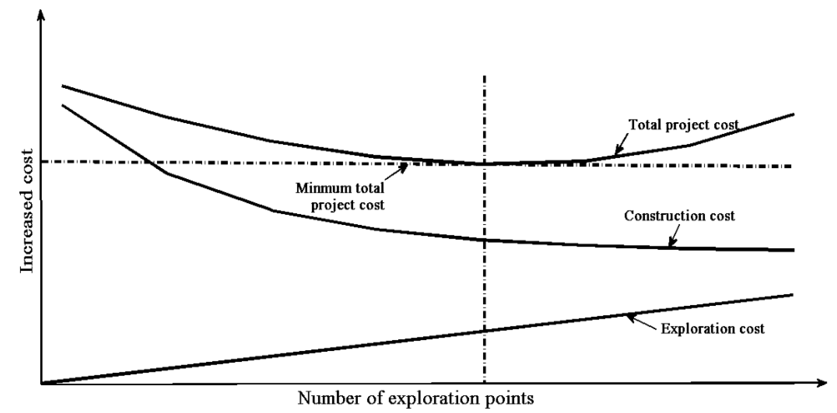
Figure 2.
Distribution and location of observation points.

Figure 3.
Probability distribution of rock types according to the original 25 observation points.
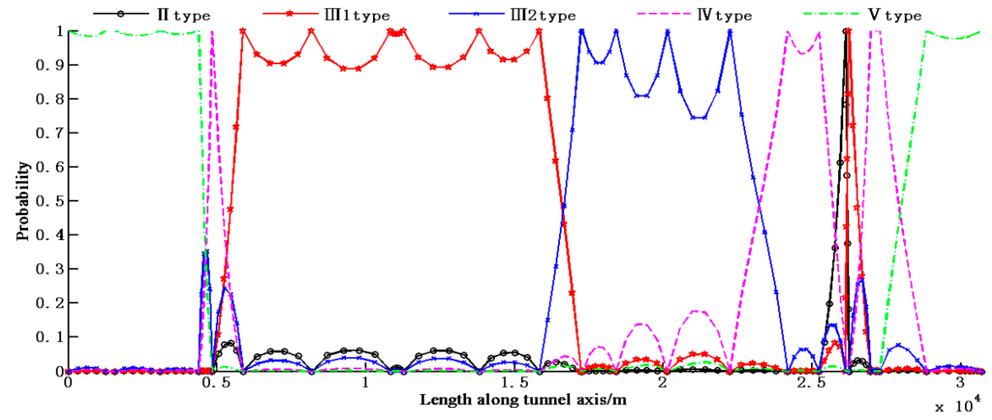
Figure 4.
Information entropy distribution according to the original 25 observation points.

Figure 5.
Probability distribution of rock types according to the new 3 observation points.

Figure 6.
Information entropy distribution according to the new 3 observation points.
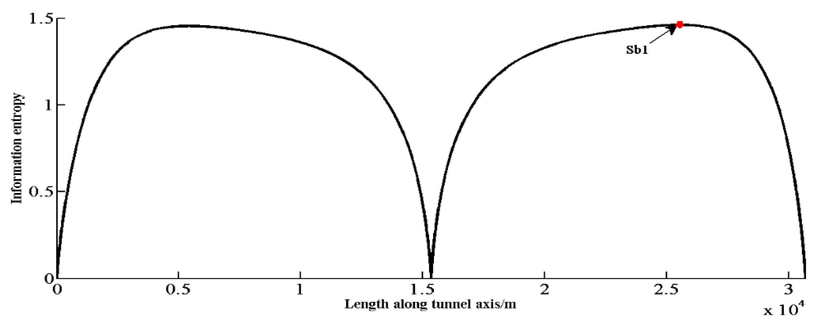
Figure 7.
Probability distribution of rock type according to the new 4 investigation points.

Figure 8.
Information entropy distribution according to the 4 new investigation points.

Figure 9.
Probability distribution of rock types according to the 25 new observation points.
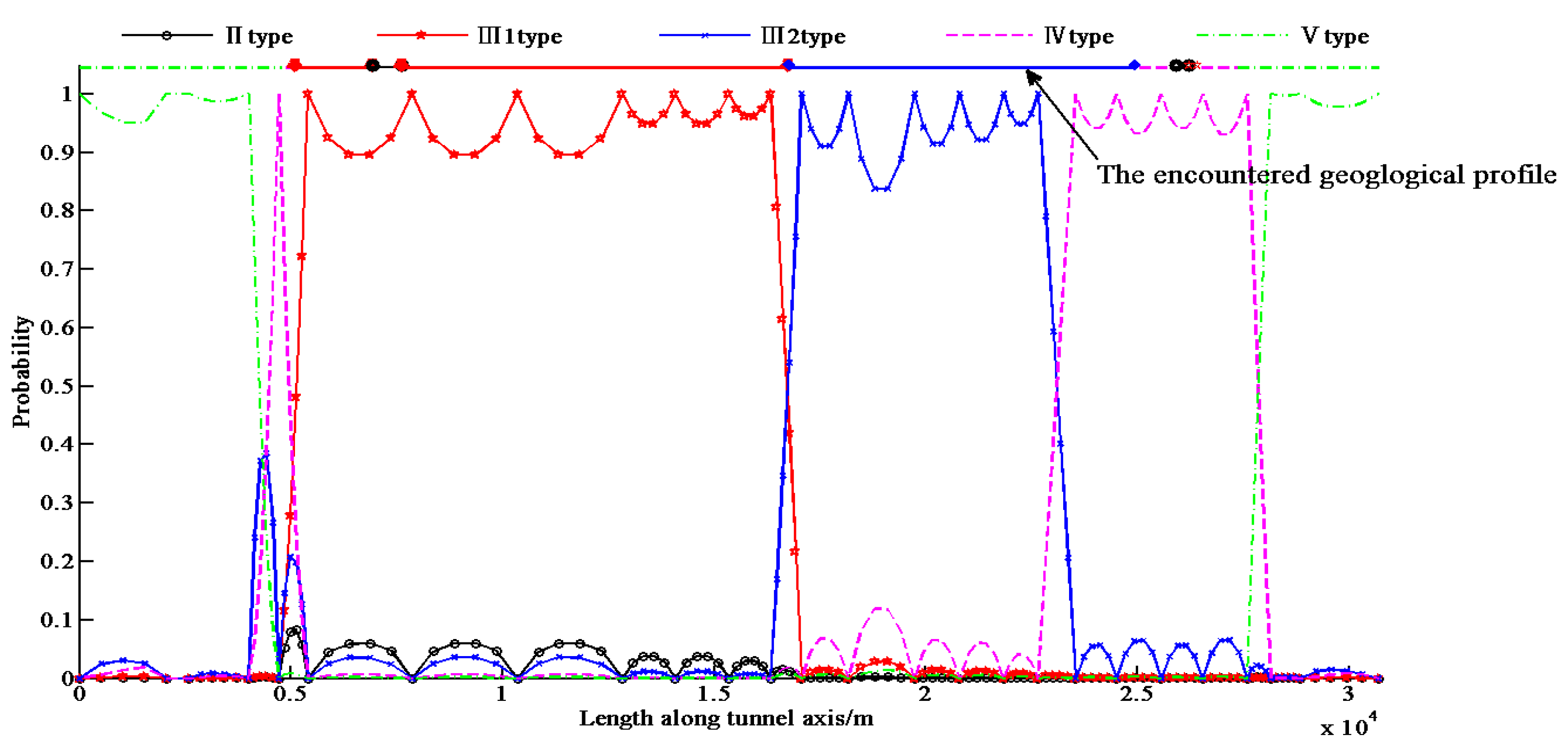
Figure 10.
Information entropy distribution according to the new 25 observation points.
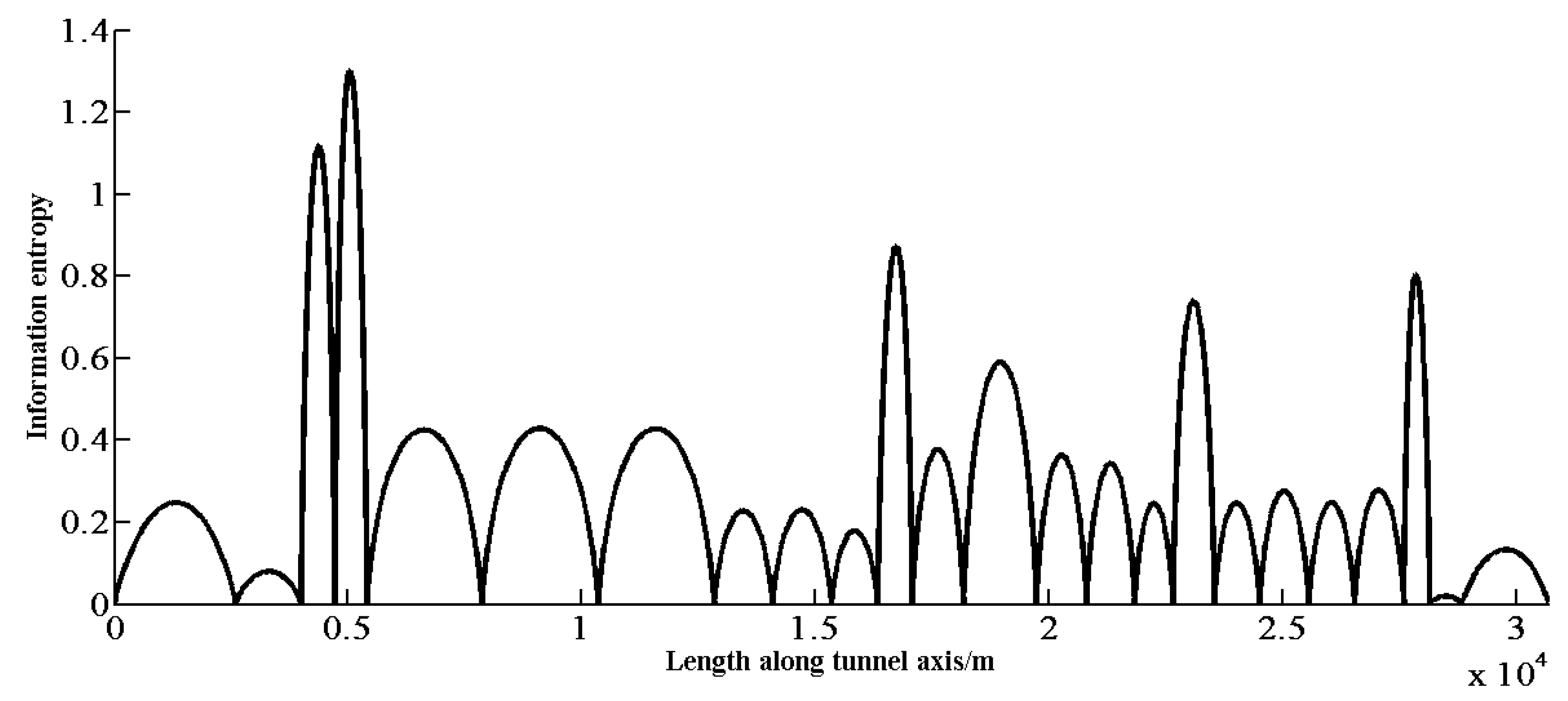
Figure 11.
Relationship between quantity and total information entropy.


Table 1.
Observation points along the Bashiyi Daban water diversion tunnel.
| Location (along the Tunnel; m) | Surrounding Rock | Location (along the Tunnel; m) | Surrounding Rock |
|---|---|---|---|
| 0 (starting point) | V type | 18,416 | III2 type |
| 1570 | V type | 20,144 | III2 type |
| 3080 | V type | 22,242 | III2 type |
| 4380 | V type | 24,187 | IV type |
| 4841 | IV type | 25,234 | IV type |
| 5880 | III1 type | 26,126 | II type |
| 8185 | III1 type | 26,239 | III1 type |
| 10,836 | III1 type | 26,974 | IV type |
| 11,264 | III1 type | 27,165 | IV type |
| 13,815 | III1 type | 27,274 | IV type |
| 15,832 | III1 type | 28,847 | V type |
| 17,230 | III2 type | 30,691 (end point) | V type |
| 17,284 | III2 type | - | - |
Table 2.
New additional observations along the Bashiyi Daban water diversion tunnel.
| Additional Quantities | Total Quantities | Optimal Location (along the Tunnel; m) | Surrounding Rock | Total Information Entropy |
|---|---|---|---|---|
| 1 | 3 | - | - | 37,129 |
| 2 | 4 | 25,566 | IV type | 35,172 |
| 3 | 5 | 5398 | III1 type | 31,665 |
| 4 | 6 | 21,837 | III2 type | 30,123 |
| 5 | 7 | 10,353 | III1 type | 26,647 |
| 6 | 8 | 19,732 | III2 type | 25,284 |
| 7 | 9 | 2580 | V type | 22,825 |
| 8 | 10 | 27,601 | IV type | 21,283 |
| 9 | 11 | 18,173 | III2 type | 20,137 |
| 10 | 12 | 23,540 | IV type | 18,943 |
| 11 | 13 | 12,836 | III1 type | 17,641 |
| 12 | 14 | 7862 | III1 type | 16,356 |
| 13 | 15 | 3999 | V type | 14,597 |
| 14 | 16 | 28,843 | V type | 13,357 |
| 15 | 17 | 17,070 | III2 type | 12,501 |
| 16 | 18 | 4711 | IV type | 12,381 |
| 17 | 19 | 16,339 | III1 type | 11,647 |
| 18 | 20 | 20,806 | III2 type | 10,906 |
| 19 | 21 | 22,661 | III2 type | 10,490 |
| 20 | 22 | 26,543 | IV type | 9928.6 |
| 21 | 23 | 24,513 | IV type | 9371.9 |
| 22 | 24 | 28,148 | V type | 8879.9 |
| 23 | 25 | 14,085 | III1 type | 8489 |
© 2017 by the authors. Licensee MDPI, Basel, Switzerland. This article is an open access article distributed under the terms and conditions of the Creative Commons Attribution (CC BY) license (http://creativecommons.org/licenses/by/4.0/).
Share and Cite
MDPI and ACS Style
Xu, C.; Hu, C.; Liu, X.; Wang, S. Information Entropy in Predicting Location of Observation Points for Long Tunnel. Entropy 2017, 19, 332. https://doi.org/10.3390/e19070332
AMA Style
Xu C, Hu C, Liu X, Wang S. Information Entropy in Predicting Location of Observation Points for Long Tunnel. Entropy. 2017; 19(7):332. https://doi.org/10.3390/e19070332
Chicago/Turabian StyleXu, Chen, Chengke Hu, Xiaoli Liu, and Sijing Wang. 2017. "Information Entropy in Predicting Location of Observation Points for Long Tunnel" Entropy 19, no. 7: 332. https://doi.org/10.3390/e19070332
Note that from the first issue of 2016, this journal uses article numbers instead of page numbers. See further details here.