Rate-Distortion Bounds for Kernel-Based Distortion Measures †


Department of Computer Science and Engineering, Toyohashi University of Technology, 1-1 Hibarigaoka Tempaku-cho Toyohashi, Aichi 441-8580, Japan
†
This paper is an extended version of my papers published in the Eighth Workshop on Information Theoretic Methods in Science and Engineering, Copenhagen, Denmark, 24–26 June 2015 and the IEEE International Symposium on Information Theory, Aachen, Germany, 25–30 June 2017.
Entropy 2017, 19(7), 336; https://doi.org/10.3390/e19070336
Submission received: 9 May 2017
/
Revised: 16 June 2017
/
Accepted: 2 July 2017
/
Published: 5 July 2017
(This article belongs to the Special Issue Information Theory in Machine Learning and Data Science)
Abstract
:Kernel methods have been used for turning linear learning algorithms into nonlinear ones. These nonlinear algorithms measure distances between data points by the distance in the kernel-induced feature space. In lossy data compression, the optimal tradeoff between the number of quantized points and the incurred distortion is characterized by the rate-distortion function. However, the rate-distortion functions associated with distortion measures involving kernel feature mapping have yet to be analyzed. We consider two reconstruction schemes, reconstruction in input space and reconstruction in feature space, and provide bounds to the rate-distortion functions for these schemes. Comparison of the derived bounds to the quantizer performance obtained by the kernel -means method suggests that the rate-distortion bounds for input space and feature space reconstructions are informative at low and high distortion levels, respectively.
1. Introduction
Kernel methods have been widely used for nonlinear learning problems combined with linear learning algorithms such as the support vector machine and the principal component analysis [1]. By the so-called kernel trick, kernel-based methods can use linear learning methods in the kernel-induced feature space without explicitly computing the high-dimensional feature mapping. Kernel-based methods measure the dissimilarity between data points by the distance in the feature space, which, in input space, corresponds to a distance measure involving the feature mapping [2]. If a kernel-based learning method is used as a lossy source coding scheme, its optimal rate-distortion tradeoff is indicated by the rate-distortion function associated with the distortion measure defined by the kernel feature map [3]. Successful applications of kernel methods in learning problems and flexibility to create various distance measures suggest that kernel-based distortion measures can be suitable for certain lossy compression problems. However, the rate-distortion function of such a distortion measure has yet to be evaluated analytically. Although there are several kernel-based approaches to vector quantization [4,5], their rate-distortion tradeoffs are still unknown.
In this paper, we derive bounds for the rate-distortion functions for kernel-based distortion measures. We consider two schemes to reconstruct inputs in lossy coding methods. One is to obtain a reconstruction in the original input space. Since kernel methods usually yield results of learning by the linear combination of vectors in feature space, we need an additional step to obtain the reconstruction in input space, such as preimaging [6]. The other is to consider the linear combination of feature vectors as the reconstruction and measure the distortion in the feature space directly. We formulate the two reconstruction schemes (Section 3.1 and Section 3.2), and prove that the rate-distortion function of input space reconstruction provides an upper bound of that of feature space reconstruction (Section 3.3). We derive lower and upper bounds to the rate-distortion function of input space reconstruction, which are computable only by -dimensional numerical integrations in the case of translation invariant and isotropic kernel functions (Section 4.1 and Section 4.2). We also provide an upper bound to the rate-distortion function of feature space reconstruction for general positive definite kernel functions (Section 4.4). In the usual applications of kernel-based quantization algorithms, one fixes the rate by determining the number of quantized points, and minimizes the average distortion for training data. The distortion-rate function, which is the inverse function of the rate-distortion function, shows the minimum achievable expected distortion (or distortion for test data) at the fixed rate. The derived bounds approximately characterize such optimal tradeoffs between the rate and expected distortion.
Furthermore, we design a vector quantizer using the kernel -means method and compare its performance with the derived rate-distortion bounds (Section 5). We also compute the preimages of the quantized points in feature space to investigate the performance of the quantizer in input space. It is suggested through the experiments using synthetic and image data that the rate-distortion bounds of reconstruction in input space are accurate at low distortion levels while the upper bound for reconstruction in feature space is informative at high distortion levels.
2. Rate-Distortion Function
Let X and Y be random variables of input and reconstruction taking values in and , respectively. For the non-negative distortion measure between x and y, , the rate-distortion function of the source is defined by
where is the mutual information and E denotes the expectation with respect to . shows the minimum achievable rate R under the given distortion measure d [3,7]. The distortion-rate function is the inverse function of the rate-distortion function and denoted by .
If the conditional distributions achieve the minimum of the following Lagrange functional parameterized by ,
then, the rate-distortion function is parametrically given by
The parameter s corresponds to the (negated) slope of the tangent of at and hence is referred to as the slope parameter [3]. Alternatively, if there exists a marginal reconstruction density that minimizes the functional,
then the optimal conditional reconstruction distributions are given by
(see, for example, [3,8]).
From the properties of the rate-distortion function , we know that for , where
and for [3] (p. 90). Hence, .
3. Kernel-Based Distortion Measures
In kernel-based learning methods, data points in input space are mapped into some high-dimensional feature space H by a feature mapping . Then, the similarity between the two points x and y in is measured by the inner product in H.
The inner product is directly evaluated by a nonlinear function in input space
which is called the kernel function. Mercer’s theorem ensures that there exists some such that Equation (4) holds if K is a positive definite kernel [1]. This enables us to avoid explicitly computing the feature map in the potentially high-dimensional space H, which is called the kernel trick. A lot of learning methods that can be expressed by only the inner products between data points have been kernelized [1].
We identify the feature space H with the reproducing kernel Hilbert space (RKHS) associated with the kernel function K by the canonical feature map, [9] (Lemma 4.19). We assume that the input space is a subset of , and the kernel function K is continuous [9] (Lemma 4.29). We focus on the squared norm in feature space as the distortion measure, and consider two reconstruction schemes in the following respective subsections.
3.1. Reconstruction in Input Space
If we restrict ourselves to the reconstruction in input space, that is, the reconstruction is computed for each input , the distortion measure is naturally defined by
Note that the reconstruction of is restricted to the subset of the feature space, . To obtain a reconstruction in input space, we need a technique such as preimaging [6].
This is a difference distortion measure if and only if the kernel function is translation invariant, that is, for any . In this case, the distortion measure is expressed as
where and . The rate-distortion function (distortion-rate function, resp.) for this distortion measure is denoted by (, resp.) and the maximum distortion in Equation (3) is denoted by , that is,
which is in the translation invariant case, .
3.2. Reconstruction in Feature Space
Suppose we have a sample of length n in input space, so that spans a linear subspace in feature space. If we compute the reconstruction by the linear combination for , and consider it as the reconstruction in feature space, the distortion can be measured by
where ,
and is the Gram matrix. Note that the reconstruction is identified with the coefficients whose domain is not identical to the input space . Although the distortion measure depends on the sample S, we omit the dependence in the notation since we consider a fixed design of S for a sufficiently large n. The sample does not have to be distributed according to the source distribution, while it is required to overspread the support of the source.
The rate-distortion function (distortion-rate function, resp.) for this distortion measure is denoted by (, resp.) and the maximum distortion in Equation (3) is given by
which is derived from the direct minimization of the quadratic function of , .
3.3. and
The following theorem claims that provides an upper bound of when n is sufficiently large.
Theorem 1.
If the input space is bounded, and there exists a conditional density achieving the infimum in the definition of , for any , , and sufficiently large n, the following inequality holds:
The proof is given in Appendix A. This theorem shows that the feature space reconstruction gives better rates since a single feature vector can be approximated by a linear combination when n is sufficiently large.
4. Rate-Distortion Bounds
Since the rate-distortion problem (Section 2) is rarely solved in a closed form [8], we derive bounds to and .
4.1. Lower Bound to
Although the Shannon lower bound to is defined for difference distortion measures in general [3] (p. 92), it diverges to for the distortion measure in Equation (6) since diverges to ∞. Hence, we consider an improved lower bound, which was introduced by [3] (p. 140). Let be the probability that . Then, is lower-bounded as
where h denotes the differential entropy,
and u is the step function. is the set of all probability densities for which for and .
In the case of the distortion measure in Equation (6), the maximum in Equation (10) is explicitly given by
where for s related to D by . Since its differential entropy is
we arrive at the following theorem.
Theorem 2.
The rate distortion function is parametrically lower-bounded as
If we further assume that the kernel function is radial, that is, for some function k, the integrations above reduce to -dimensional ones,
and
where is the area of the m-dimensional unit sphere, and is the gamma function.
4.2. Upper Bound to
If in Equation (5) is a difference distortion measure, that is, K is translation invariant, by choosing for the density in Equation (12), the following upper bound is obtained,
where is given by Equation (13) and is the convolution between and p. This type of upper bound was used to prove the asymptotic tightness of the Shannon lower bound (as ) for a class of general sources and distortion measures [3,10,11,12]. However, this upper bound requires the evaluation of the differential entropy of the convolution.
The following theorem is derived from the facts that the spherical Gaussian distribution maximizes the entropy under the constraint that is no greater than a constant, and that holds for .
4.3. Rate-Distortion Dimension
In this section, we evaluate the rate-distortion dimension [13] of the kernel-based distortion measure in Equation (5) to investigate its property. We focus on the radial kernel, , also in this section, and assume that
holds for some and . For example, the Gaussian kernel, , satisfies Equation (19) for and .
To examine the limit of , we consider the asymptotic case of . Since , it follows that
and
Thus, we have from Equations (14) and (17),
for both the lower and upper bounds, and from Equation (13),
Since in Equation (5) is a norm squared for a valid RKHS kernel K, the rate-distortion dimension of the source distribution p is defined by [13],
From Theorems 2 and 3 and Equation (20), we conclude the following.
Theorem 4.
This theorem shows that the rate-distortion dimension is dependent only on the dimensionality of the input space and independent of the dimensionality of the feature space. In the case of the linear kernel, , with , the distortion measure in Equation (5) reduces to the usual squared distortion measure, . It can be shown that under norm-based distortion measures including the squared distortion measure, the rate-distortion dimension of a source with an m-dimensional density is m [11,12]. From the preceding theorem, this is also the case for a general radial kernel if the kernel function has the order as the Gaussian kernel. Expression (22) of the rate-distortion dimension will be examined through a numerical experiment in Section 5.1.
4.4. Upper Bound to
We construct an upper bound to the rate-distortion function . We choose the conditional distribution of the reconstruction by
where ,
and denotes the n-dimensional normal density with mean and covariance matrix . Here, we have introduced the regularization constant with the identity matrix . The conditional distribution in Equation (23) is implied by Equation (2) and the approximation . This reconstruction distribution yields the following upper bound:
where ,
which is independent of the input x, and
If , is the mean of the variance of the prediction by the associated Gaussian process [14].
Further upper-bounding the differential entropy by the Gaussian entropy, we have the following theorem.
Theorem 5.
The rate distortion function is upper-bounded as
where
The proof is put in Appendix B. In the simplest case where , , and the source is the Gaussian, , the upper bound in Equation (27) reduces to
which is an asymptotically (as ) tight upper bound of the well-known rate distortion function for the Gaussian source under the squared distortion measure, [3,7].
5. Experimental Evaluation
We numerically evaluate the rate-distortion bounds obtained in the previous section. Designing a quantizer by the kernel -means algorithm, we compare its performance with the bounds.
We focus on the case of the Gaussian kernel,
with the kernel parameter .
5.1. Synthetic Data
As a source, we first assumed the uniform distribution on the union of the two regions, and , where and have equal volumes and has volume 1. This suggests that and in Equation (10) and succeeding equations in Section 4.1 and Section 4.2.
We used the trapezoidal rule to compute the -dimensional integrations in the lower bound and the upper bound . We generated i.i.d sample of the size from the source to compute and for in Equation (27). Generating another 4000 data points, we approximated the required expectations. We optimized the regularization coefficient c to minimize the upper bound for each D.
Using the same data set of the size 4000 as a training data set, we run the kernel -means algorithm 10 times with random initializations to obtain the minimum distortion for each rate. Varying the number of quantized points from to , for each , we counted the effective number of quantized points which have at least one assigned data point and computed the rate by as the quantizer is first order, that is, the block length is one. The kernel parameter was chosen so that the clear separation of and is obtained when .
After the training, we computed the distortion and rate for the test data set, by assigning each of 20,000 test data generated from the same source to the nearest quantized points in the feature space.
For each quantized point, we obtained its preimage. That is, if the kth quantized point is expressed as , its preimage is
We used the mean shift procedure for the maximization, although this procedure only guarantees the convergence to a local maximum [15,16].
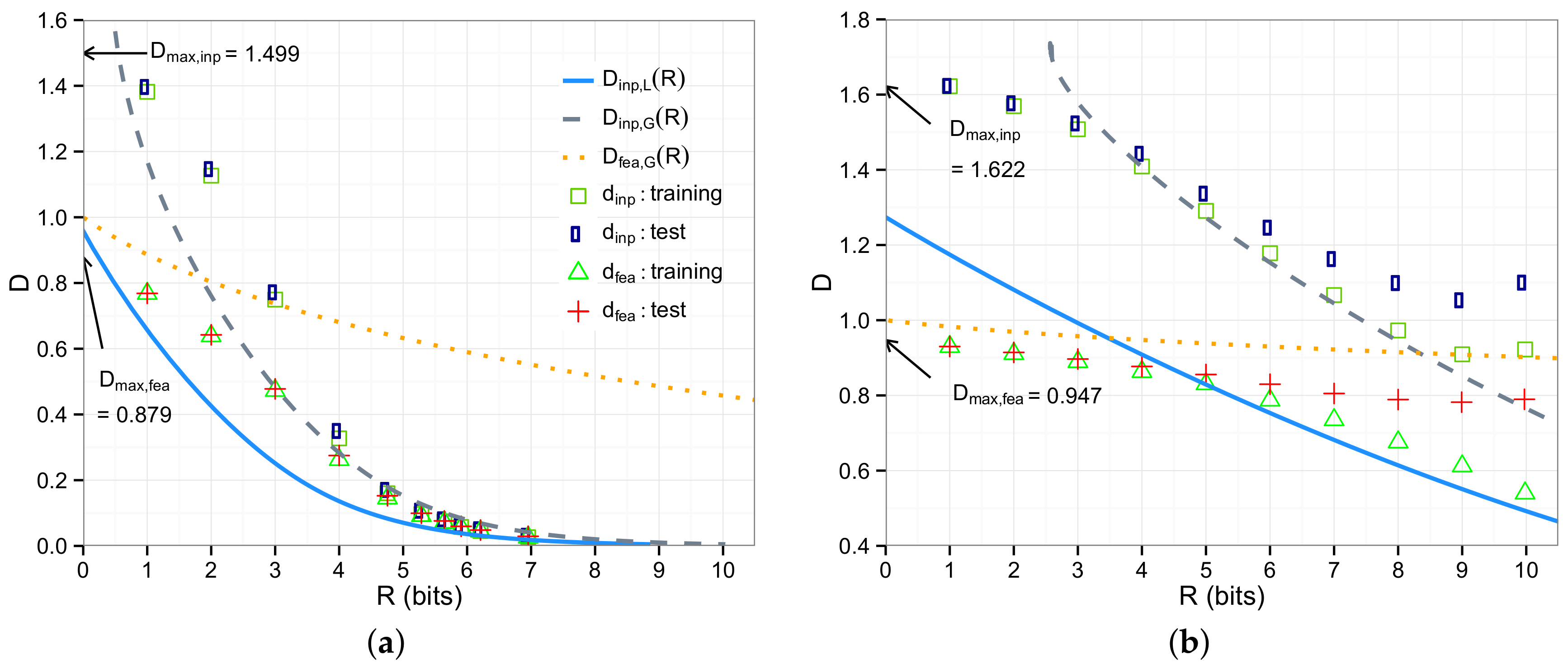
The obtained bounds and the quantizer performances are displayed in Figure 1a,b and for and , respectively, in the forms of distortion-rate functions. The values of in Equations (7) and (9) are also indicated in the figures.
In both dimensions, the upper bound is smaller than at low rates while the bound is above the quantizer performance. However, the value of suggests that the bound is informative at low rates. As the rate becomes higher, the lower and upper bounds of the input space reconstruction, and , approach each other. In fact, they sandwich the quantizer performance tightly in the -dimensional case, which suggests that the rate-distortion function for the feature space reconstruction, is close to the rate-distortion function of the input space reconstruction at high rates.
We see that the quantizer performances for and those for approach each other as the rate R grows. The upper bound reasonably approximates the quantizer performance by the preimages, and it indicates that, in the -dimensional case (Figure 1a), the results for and 3 bits can be improved by at least about 1 bit.
At low distortion levels, each source output should be reconstructed within a small neighborhood in the feature space where we can find another point y in the input space whose feature map is sufficiently close to the reconstruction. This suggests that the rate-distortion function of feature space reconstruction is well approximated by the rate-distortion function of input space reconstruction. In other words, combining multiple input points to make a reconstruction in feature space does not do any good for reducing distortion and only a single input point is enough when it is mapped into feature space. Hence, the rate-distortion bounds of input space reconstruction may be informative at low distortion levels.
In the 10-dimensional case (Figure 1b), the distortion in the test data set is close to or above it at high rates. This may be due to overfitting of the kernel -means to the training data set of the size, 4000. That is, as the the rate grows, the distortion in the training data set decreases and the discrepancy between the distortions in the training and test sets increases.
To examine the asymptotic behavior of discussed in Section 4.3, we computed and for small D, that is, for large s. As well as the Gaussian kernel Equation (29), which has in Equation (19), we applied the Laplacian kernel,
which corresponds to . The kernel parameter of the Laplacian kernel was set to the square root of the value used in the Gaussian kernel.
The rate-distortion bounds, and divided by for small distortion levels are shown in Figure 2a,b and for and , respectively. We can see that, in each case, the ratio tends to , that is, the rate-distortion dimension evaluated in Equation (22) as . For the distortion levels smaller than those presented in Figure 2, the ratios start oscillating due to the errors of numerical integrations.
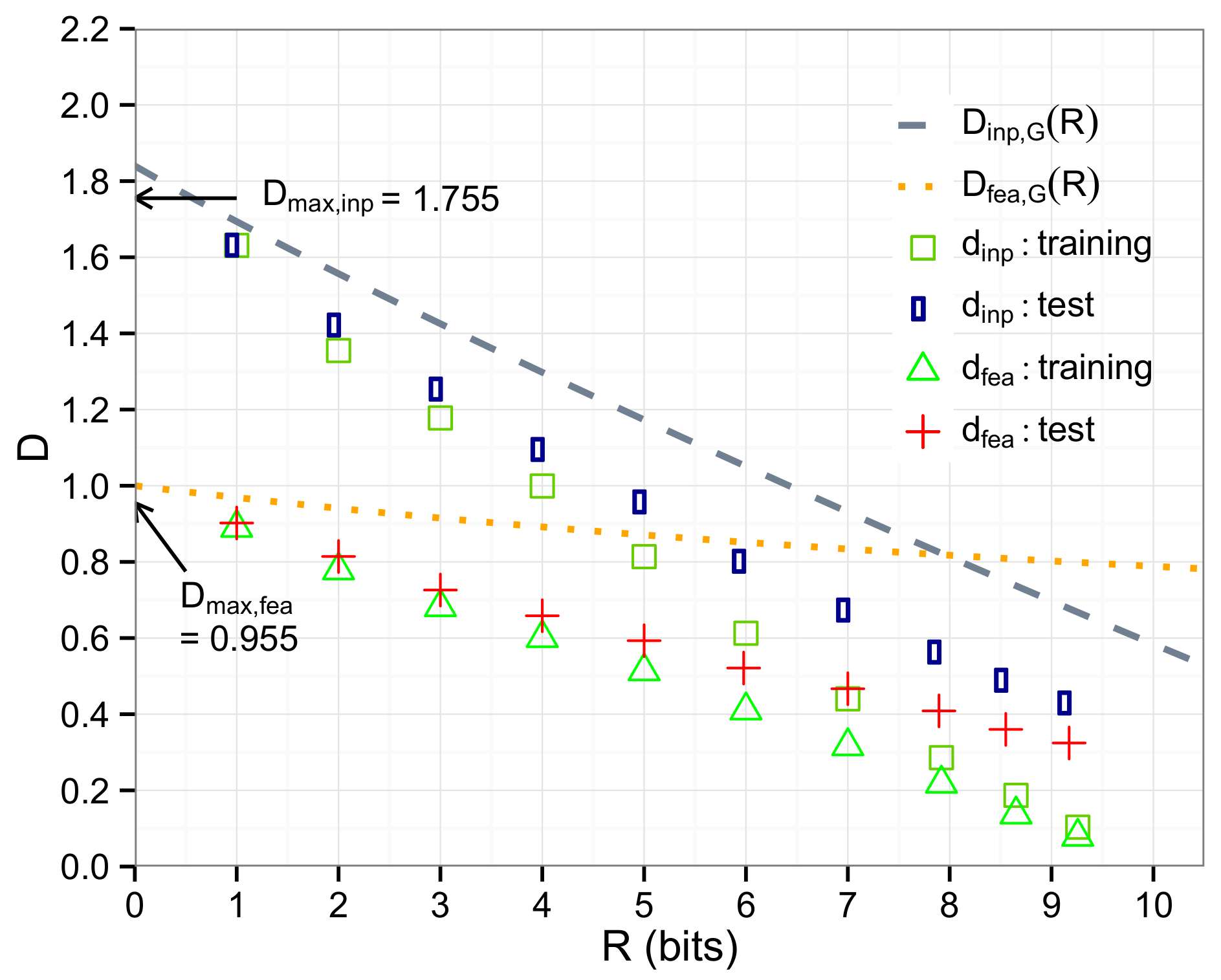
5.2. Image Data
We carried out a similar evaluation of the rate-distortion bounds and quantizer performances for a grayscale image data set extracted from the COIL20 data set [18]. We used the first category from 20 categories of images, which consisted of 72 images of size . Dividing each image into small patches of size (), we obtained 256 data from each image, and 18,432 data in total. Removing duplicate data points, we finally obtained 13,368 data. We used first 2048 data as the training data and the remaining 11,320 data as the test data. The training data set was also used for approximating expectations of kernel functions required to compute , and the first data points were used as the sample data in the definition of . We evaluated only the upper bounds, and , since the lower bound requires estimating the source entropy from empirical data, which depends heavily on the estimation method, and hence is to be addressed more in detail.
Each dimension was normalized so that it has mean 0 and variance 1. Hence, in was approximated by the empirical variance, 1. The boundary B in was approximated by the maximum norm of the training data points.
The upper bounds and quantizer performances are presented in Figure 3. Although the upper bounds are loose and above the respective quantizer performances, the upper bound is roughly predictive of the quantizer performance in the input space, and so does for the reconstruction in the feature space.
6. Conclusions
In this paper, we have shown upper and lower bounds for the rate-distortion functions associated with kernel feature mapping. As suggested in Section 5, the upper bound for the reconstruction in feature space is informative at high distortion levels while the bounds for the reconstruction in input space are informative at low distortion levels. We have also evaluated the rate-distortion dimension of sources with bounded support under kernel-based distortion measures, which shows the asymptotic behavior of the rate-distortion function. Our future directions include deriving tighter bounds and exact evaluation of the rate-distortion function in some special cases. In particular, it is an important undertaking to derive a lower bound to the rate-distortion function of the reconstruction in feature space.
Acknowledgments
The author would like to thank the anonymous reviewers for their helpful comments and suggestions. This work was supported in part by the Japan Society for the Promotion of Science (JSPS) grants 25120014, 15K16050, and 16H02825.
Conflicts of Interest
The author declares no conflict of interest.
Appendix A. Proof of Theorem 1
Proof.
Let be the conditional density for that achieves the infimum of . Then, for , it holds that and
Since the input space is bounded and separable, and the kernel function K is continuous, for any and , there exist coefficients such that
holds when n is sufficiently large.
Appendix B. Proof of Theorem 5
References
- Schölkopf, B.; Smola, A.J. Learning with Kernels: Support Vector Machines, Regularization, Optimization, and Beyond; MIT Press: Cambridge, MA, USA, 2001. [Google Scholar]
- Aizerman, M.A.; Braverman, E.A.; Rozonoer, L. Theoretical foundations of the potential function method in pattern recognition learning. Autom. Remote Control 1964, 25, 821–837. [Google Scholar]
- Berger, T. Rate Distortion Theory: A Mathematical Basis for Data Compression; Prentice-Hall: Englewood Cliffs, NJ, USA, 1971. [Google Scholar]
- Girolami, M. Mercer kernel-based clustering in feature space. IEEE Trans. Neural Netw. 2002, 13, 780–784. [Google Scholar] [CrossRef] [PubMed]
- Filippone, M.; Camastra, F.; Masulli, F.; Rovetta, S. A survey of kernel and spectral methods for clustering. Pattern Recognit. 2008, 41, 176–190. [Google Scholar] [CrossRef]
- Schölkopf, B.; Mika, S.; Burges, C.J.C.; Knirsch, P.; Müller, K.R.; Ratsch, G.; Smola, A.J. Input space versus feature space in kernel-based methods. IEEE Trans. Neural Netw. 1999, 10, 1000–1017. [Google Scholar] [CrossRef] [PubMed]
- Cover, T.M.; Thomas, J.A. Elements of Information Theory; Wiley Interscience: Hoboken, NJ, USA, 1991. [Google Scholar]
- Gray, R.M. Entropy and Information Theory, 2nd ed.; Springer: Berlin/Heidelberg, Germany, 2011. [Google Scholar]
- Steinwart, I.; Christmann, A. Support Vector Machines; Springer: Berlin/Heidelberg, Germany, 2008. [Google Scholar]
- Linkov, Y.N. Evaluation of ϵ-entropy of random variables for small ϵ. Probl. Inf. Transm. 1965, 1, 18–26. [Google Scholar]
- Linder, T.; Zamir, R. On the asymptotic tightness of the Shannon lower bound. IEEE Trans. Inf. Theory 1994, 40, 2026–2031. [Google Scholar] [CrossRef]
- Koch, T. The Shannon lower bound is asymptotically tight. IEEE Trans. Inf. Theory 2016, 62, 6155–6161. [Google Scholar] [CrossRef]
- Kawabata, T.; Dembo, A. The rate-distortion dimension of sets and measures. IEEE Trans. Inf. Theory 1994, 40, 1564–1572. [Google Scholar] [CrossRef]
- Rasmussen, C.E.; Williams, C.K.I. Gaussian Processes for Machine Learning (Adaptive Computation and Machine Learning); The MIT Press: Cambridge, MA, USA, 2005. [Google Scholar]
- Fukunaga, K.; Hostetler, L. The estimation of the gradient of a density function, with applications in pattern recognition. IEEE Trans. Inf. Theory 1975, 21, 32–40. [Google Scholar] [CrossRef]
- Comaniciu, D.; Meer, P. Mean shift: A robust approach toward feature space analysis. IEEE Trans. Pattern Anal. Mach. Intell. 2002, 24, 603–619. [Google Scholar] [CrossRef]
- Watanabe, K. Rate-distortion analysis for kernel-based distortion measures. In Proceedings of the Eighth Workshop on Information Theoretic Methods in Science and Engineering, Copenhagen, Denmark, 24–26 June 2015. [Google Scholar]
- Nene, S.A.; Nayar, S.K.; Murase, H. Columbia Object Image Library (COIL-20). Available online: http://www.cs.columbia.edu/CAVE/software/softlib/coil-20.php (accessed on 4 July 2017).
Figure 1.
Rate-distortion bounds and quantizer performances for (a) and (b) [17].
Figure 1.
Rate-distortion bounds and quantizer performances for (a) and (b) [17].

Figure 2.
The ratios between the rate-distortion bounds and for (a) and (b) . The bounds are for the Laplacian kernel () and the Gaussian kernel ().
Figure 2.
The ratios between the rate-distortion bounds and for (a) and (b) . The bounds are for the Laplacian kernel () and the Gaussian kernel ().
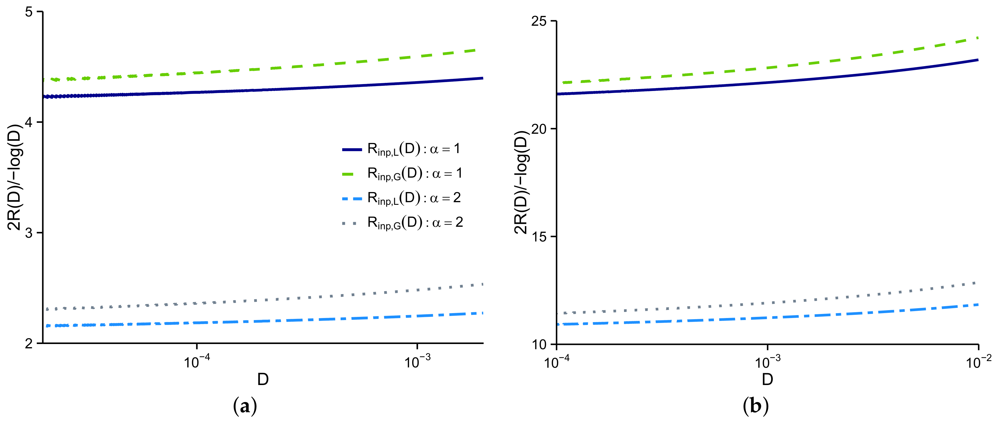
Figure 3.
Upper bounds of the rate-distortion functions and quantizer performance for image data.
© 2017 by the author. Licensee MDPI, Basel, Switzerland. This article is an open access article distributed under the terms and conditions of the Creative Commons Attribution (CC BY) license (http://creativecommons.org/licenses/by/4.0/).
Share and Cite
MDPI and ACS Style
Watanabe, K. Rate-Distortion Bounds for Kernel-Based Distortion Measures. Entropy 2017, 19, 336. https://doi.org/10.3390/e19070336
AMA Style
Watanabe K. Rate-Distortion Bounds for Kernel-Based Distortion Measures. Entropy. 2017; 19(7):336. https://doi.org/10.3390/e19070336
Chicago/Turabian StyleWatanabe, Kazuho. 2017. "Rate-Distortion Bounds for Kernel-Based Distortion Measures" Entropy 19, no. 7: 336. https://doi.org/10.3390/e19070336
Note that from the first issue of 2016, this journal uses article numbers instead of page numbers. See further details here.