A Novel Feature Extraction Method for Ship-Radiated Noise Based on Variational Mode Decomposition and Multi-Scale Permutation Entropy


School of Marine Science and Technology, Northwestern Polytechnical University, Xi’an 710072, China
*
Authors to whom correspondence should be addressed.
Entropy 2017, 19(7), 342; https://doi.org/10.3390/e19070342
Submission received: 28 June 2017
/
Revised: 5 July 2017
/
Accepted: 6 July 2017
/
Published: 8 July 2017
(This article belongs to the Section Complexity)
Abstract
:In view of the problem that the features of ship-radiated noise are difficult to extract and inaccurate, a novel method based on variational mode decomposition (VMD), multi-scale permutation entropy (MPE) and a support vector machine (SVM) is proposed to extract the features of ship-radiated noise. In order to eliminate mode mixing and extract the complexity of the intrinsic mode function (IMF) accurately, VMD is employed to decompose the three types of ship-radiated noise instead of Empirical Mode Decomposition (EMD) and its extended methods. Considering the reason that the permutation entropy (PE) can quantify the complexity only in one scale, the MPE is used to extract features in different scales. In this study, three types of ship-radiated noise signals are decomposed into a set of band-limited IMFs by the VMD method, and the intensity of each IMF is calculated. Then, the IMFs with the highest energy are selected for the extraction of their MPE. By analyzing the separability of MPE at different scales, the optimal MPE of the IMF with the highest energy is regarded as the characteristic vector. Finally, the feature vectors are sent into the SVM classifier to classify and recognize different types of ships. The proposed method was applied in simulated signals and actual signals of ship-radiated noise. By comparing with the PE of the IMF with the highest energy by EMD, ensemble EMD (EEMD) and VMD, the results show that the proposed method can effectively extract the features of MPE and realize the classification and recognition for ships.
1. Introduction
Ships are important equipment in the marine field. Ship-radiated noise can reflect some important physical properties of ships, so the research of ship-radiated noise is of great significance. Feature extraction of ship-radiated noise is one of the key problems in the field of underwater acoustic signal processing and plays a significant role in research and practical application. Ambient noise, which is constituted by contributions from numerous natural and anthropogenic sources, has made it difficult to extract the features of ships that can reflect properties of the ship from the ship-radiated noise [1,2]. As a result, accurate feature extraction of ship radiated-noise becomes a very challenging work by traditional analysis in the time and frequency domains. For example, Fourier transform analysis cannot reflect time-varying characteristics of the signal well; also, the wavelet transform can provide signal time-frequency information at the same time, while it is limited by the selection of the wavelet basis function [3].
The Empirical Mode Decomposition (EMD) [4,5] method was put forward by Huang et al. in 1998. The EMD is completely self-adaptive and a data-driven method that is based on the scale characteristics of the signal itself. The intrinsic mode function (IMF) obtained by EMD can represent the real physical meaning of the signal, and it can also reflect the real physical characteristics of the system. The EEMD [6] method is an improved EMD method, which can effectively solve the problem of mode mixing. However, EMD, and its extended methods, are empirical algorithms and sensitive to noise, without a solid theoretical foundation in mathematics. In contrast to EMD and EEMD, variational mode decomposition (VMD) [7,8], first introduced by Dragomiretskiy et al., is a non-recursive method to analyze non-linear and non-stationary signals, which can adaptively decompose signals into a number of quasi-orthogonal IMFs. Each IMF is compact around a center frequency which can be estimated online. In addition, some studies show the VMD is superior to EMD and its extended methods in noise robustness, signal decomposition, and extraction.
With the development of the theory and practice of VMD, EMD, and its extended methods, they have been widely applied in the fields of fault diagnosis [9,10], biomedical science [11,12], geophysics [13], and underwater acoustic signal processing [14,15,16,17]. For example, research in [9] an EEMD-based methods for fault diagnosis of rotating machinery is proposed and applied to rub-impact fault diagnosis of a power generator and early rub-impact fault diagnosis of a heavy oil catalytic cracking machine set. In [16], the centre frequency of IMF with the highest energy by EEMD constructed a new characteristic parameter that can distinguish different types of ships. In [18], a denoising method, which combines VMD and detrended fluctuation analysis, addresses the selection of the number of modes. In addition, it shows low computational cost and the superior denoising performance on simulated and real signals. Research in [10] investigated the equivalent filtering characteristics of VMD, and proved that the multiple features can be better extracted with the VMD for rotor-stator fault diagnosis. Research in [19] investigated features of VMD illustrated three potential applications of VMD in extracting time-varying oscillations, detrending, as well as detecting impacts. Most of the above proved the feasibility and effectiveness of these decomposition methods for feature extraction. Moreover, VMD showed some advantages over EMD and EEMD in some studies.
Permutation entropy (PE) [20], as a nonlinear dynamics parameter, is a powerful tool which can describe the complexity of a time series. It only takes into account the temporal information in the time series, thus, it has the advantages of simple calculation, strong anti-noise ability, robustness, and low computational cost. MPE [21,22], which is based on PE, can describe the complexity of time series in different scales. Many studies have extracted features of signals by PE combining VMD, EMD, or EEMD in the fields of medicine [23,24,25], fault diagnosis [26,27,28,29,30], and underwater acoustic signal processing [31]. In [24], the energy, the renyi entropy, and the PE of the first three modes are calculated and used as diagnostic features by VMD, and experimental results show that the proposed method can distinguish accurately between shockable ventricular arrhythmia and non-shockable ventricular arrhythmia by a classifier. In [27], the PE of the first five IMFs by EEMD are regarded as the feature of a vibration signal, and optimized support vector machines are used to classify the fault type and severity; simulation results demonstrate that the proposed approach can effectively distinguish the fault type with high accuracy for motor bearing faults. In [28], a novel method of fault diagnosis for rolling bearings based on VMD, PE, and SVM is put forward, and PEs of all the IMFs by VMD are regarded as the characteristic vector, the comparison results showing that the proposed method outperforms the method bases on EMD and PE. However, few studies have extracted features of signals by MPE combining VMD, EMD, or EEMD in many fields.
In recent years, many scholars have conducted much research on the feature extraction of ship-radiated noise. In [14], the statistic centre frequency of eight IMFs by EMD construct a characteristic vector, which can achieve higher discrimination for different types of ships. Moreover, research in [15] extracts the energy difference between the high- and low-frequency characteristics from different ship-radiated noise signals by EEMD. In [31], PE is first used to extract features of ship-radiated noise combining EMD, and the proposed method has better separability than [15]. However, as far as we know, few studies have extracted features of signals by VMD combining MPE in the field of underwater acoustic signal processing.
In this paper, based on the above analysis, a new method for feature extraction of ship-radiated noise is presented by taking advantage of the VMD and MPE. The outline of this paper is as follows: Section 1 is the introduction; Section 2 is the basic theory of VMD and MPE; in Section 3, the review of the proposed method for feature extraction of ship-radiated noise is presented; in Section 4, the proposed method is applied to simulation experimental data; in Section 5, the proposed method is applied to ship-radiated noise signals; and, finally, Section 6 is the conclusion.
2. Basic Theory
2.1. VMD Method
VMD is a new multi-component signal decomposition algorithm based on Wiener filtering, Hilbert transform, and heterodyne demodulation. Unlike EMD and its extended algorithms, it defines the IMF as an amplitude-modulated-frequency-modulated (AM-FM) signal as follows:
where the envelope and instantaneous frequency are nonnegative. In addition, the change of and are more slower than . Each is compact around a respective centre frequency, and its bandwidth is obtained by means of Gauss smooth demodulation. When VMD is used to non-recursively decomposed multi-component signal, the constrained variational problem is defined as:
where denotes the number of the IMF, is the input signal, indicates each IMF, and represents the centre frequency of each IMF. In order to solve the constrained problem to Equation (2), the penalty parameter and the Lagrange multiplication operator are applied to change Equation (2) to the non-constraint problem. The augmented Lagrange is denoted as:
where is regarded as the balancing parameter of the data-fidelity constraint. By using the alternating direction multiplier method (ADMM), the saddle point of Equation (3) can be obtained and the estimated , corresponding centre frequency , and are updated in the frequency domain, which can be written as follows:
where is the update parameter. There are two different methods for setting the initialization of centre frequencies, namely, uniformly spaced distribution and zero initial. Specifically, the uniformly-spaced distribution for the centre frequency is defined as:
while the zero initial can be represented simply by:
The specific process of the VMD algorithm is summarized as follows:
- (1)
- Initialize , , , and n = 0.
- (2)
- Updated the value of and according to Equations (4)–(6).
- (3)
- Judge whether or not meets the convergence condition in Equation (9):
Repeat the process of (2) until the convergence stop condition is satisfied, where is the accuracy for convergence. The complete algorithm and the implementation of VMD can be found in [7].
2.2. Analysis of the Simulation Signal Based on VMD
To prove the validity of the VMD method, the decomposition of simulation signal is performed by EMD, EEMD, and VMD. The simulation signals are as follows:
where , , , and represent the four components of . EMD, EEMD, and VMD are used to decompose . The simulation signals and the decomposition result of EMD, EEMD, and VMD are presented in Figure 1. The sampling frequency is 10 kHz.
As it can be seen in Figure 1, EMD and EEMD separated into six and eight IMFs, which is more than the four components of . There is a certain degree of mode mixing by EMD and EEMD. However, when the number of decompositions is 4, VMD separated into four IMFs, and there is a consistent one-to-one match between each IMF and each component of . The correlation coefficients of the simulation signals and corresponding IMFs are shown in Table 1. As seen in Table 1, the simulation signal has no corresponding IMF by EMD, and the correlation coefficients by VMD are greater than the correlation coefficients by EMD and EEMD. It can be concluded that the VMD method is more efficient.
2.3. PE Method
The principle of PE was described in detail in [20]. Mathematically, the phase space of a time series can be constructed as:
where is the time delay and is the embedded dimension which determines the quantity of elements in the row vector of the matrix. Each row vector in the matrix can be regarded as a reconstruction component. The matrix consists of reconstruction row vector which is equal to . Each row vector can be arranged in an increasing order as:
if two elements in a vector have the same value as:
Their original order can be rearranged as:
Consequently, for any time sequence, each row vector has a group of symbol sequences as:
where , and , phase space with m dimensions has different symbol sequences , and symbol sequence is just one of the symbol permutations. If the probability of each symbol sequence is expressed as , then the PE of order for time sequences can be defined as:
when , the value of is (maximum value). For convenience, can be normalized as:
where the value of shows the degree of randomness of time sequence. A lower value shows more regular time sequence; while higher value indicates less regular time sequence. In this paper, the setting value of parameters of PE was the same with [28].
2.4. MPE Method
MPE is a kind of improvement based on PE. Its fundamental idea is to calculate the PE of the coarse-grained time sequence. The process of coarse graining for the time sequence whose length is L can be defined as:
where is the scale factor, and is the multi-scale time sequence. When the scale factor is 1, the time sequence is the original time sequence, and its MPE is the PE. After coarse-grained processing, the new time sequence can be used to calculate the MPE according to the PE method. The process of coarse-graining is important in the analysis of MPE, in which the time sequence is divided into sections and each section is equalized to obtain a new time sequence. Therefore, the selection of the scale factor is crucial in the analysis of the complexity of signals.
To compare the differences between the PE and MPE, the analysis of simulation signals is performed. The simulation signals are as follows:
where , , and represent the three simulation signals. The time delay and the embedded dimension are 1 and 3, respectively. The scale factor is from 1 to 10. The sampling frequency and data length are set as 1 kHz and 5000, respectively. The MPE of the simulation signals are presented in Figure 2.
As it can be seen in Figure 2, the PE, when the scale factor is 1, is very close for the three simulation signals. However, when the scale factor is greater than 1, there are some differences in MPE for the three simulation signals, especially when the scale factor is 10.
3. Feature Extraction Method Based on VMD and MPE
The key to feature extract is choosing the appropriate decomposition method to identify the type of signal. VMD has a strong ability of analysis in the time-frequency domain and widely used in many fields. Combined with the property of the MPE, a hybrid feature extraction approach can be designed as shown in Figure 3. The main steps are as follows:
Step 1: The three types of ship-radiated noise signals are sampled and then normalized. Additionally, the number of decompositions is selected according to the result of EMD. Then, we can obtain all the IMFs by VMD.
Step 2: The intensities of IMFs are calculated, and the optimal IMFs with the highest energy are selected to represent the original ship-radiated noise signals.
Step 3: The parameters of MPE are selected, and the MPE of the optimal IMF is calculated at different scales. After analysis and comparison, the optimal feature, which is easy to distinguish the four types of ship-radiated noise signals, is selected as the characteristic vector.
Step 4: Calculate the optimal features of 50 samples for each type of ship-radiated noise, and send them into the SVM as the training set and testing set. Then, we can obtain the classification results of three types of ship-radiated noise signals by SVM.
4. Analysis of Simulation Signal Based on VMD and MPE
4.1. The VMD of Simulation Signal
In order to verify the accuracy of MPE of IMF by VMD, the decomposition of simulation signal is performed by EMD, EEMD, and VMD. The simulation signals are as follows:
where , , and represent the three components of the simulation signal . , , . is the standard Gaussian white noise, is the noisy signal containing both and . The sampling frequency and data length are set as 1 kHz and 1000. The simulation signals and the decomposition results of EMD, EEMD, and VMD are presented in Figure 4.
As it can be seen in Figure 4, the first two IMFs are the noise modes for EMD and EEMD methods, and we can find the IMFs corresponding to , , and for the three decomposition methods; their correspondence is shown in Table 2. Compared with the EMD and EEMD methods, the VMD result is closer to the original simulation signal.
4.2. The MPE of IMF with the Highest Energy
The average intensity of each IMF can be calculated, and then the IMF with the highest energy can be obtained. In addition, before calculating the average intensity of each IMF, the noise modes should be removed for EMD and EEMD methods. The IMF with the highest energy corresponds to the simulation signal S1 for the three decomposition methods, the MPE of them is shown in Table 3. As seen in Table 3, compared with the EMD and EEMD methods, the MPE of IMF with the highest energy by VMD is closer to the MPE of simulation signal S1 in the scale from 1 to 2. Therefore, the MPE of IMF with the highest energy by the VMD method is more accurate than the EMD and EEMD methods.
5. Feature Extraction of Ship-Radiated Noise Based on VMD and MPE
5.1. The VMD of Ship-Radiated Noise
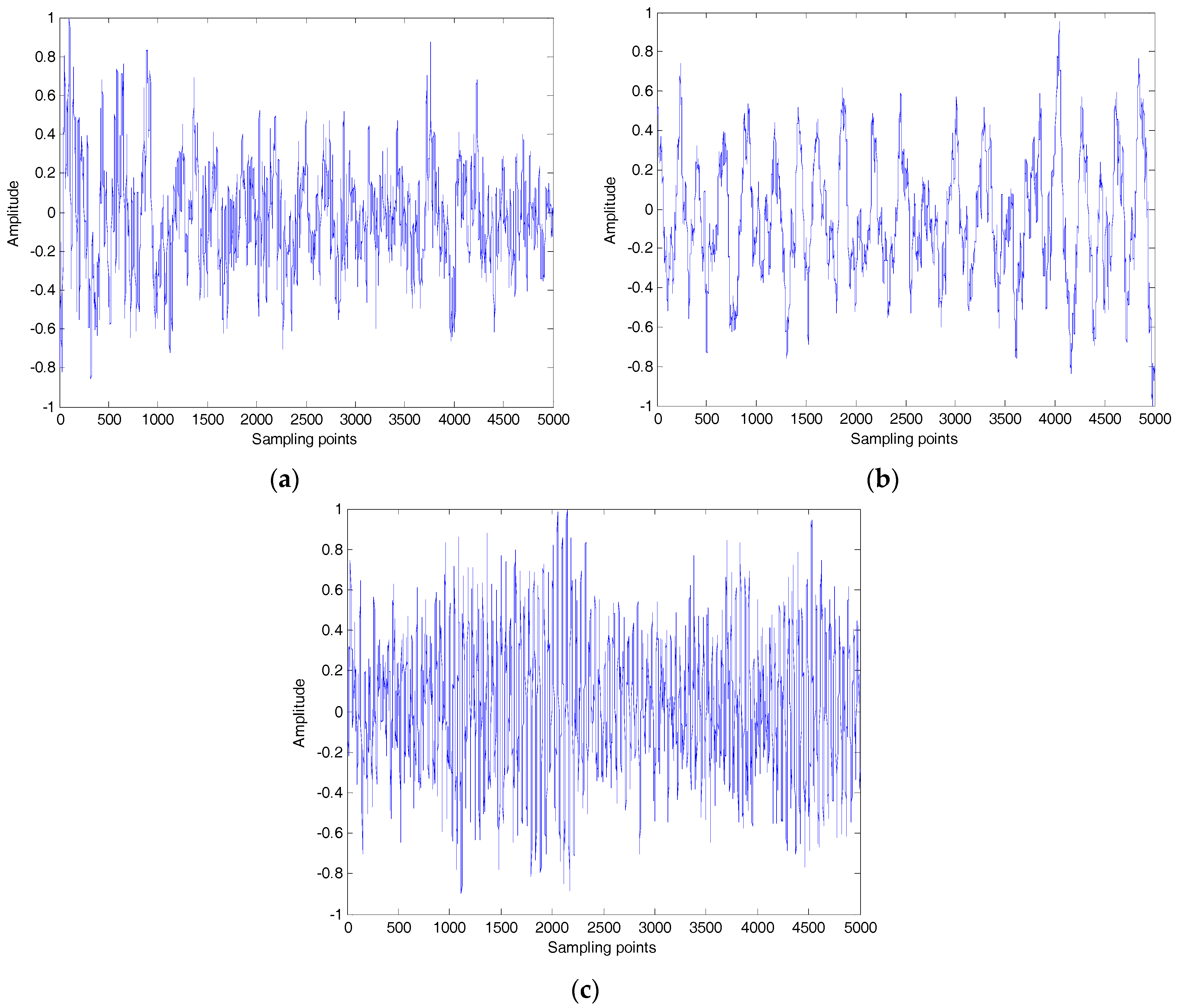
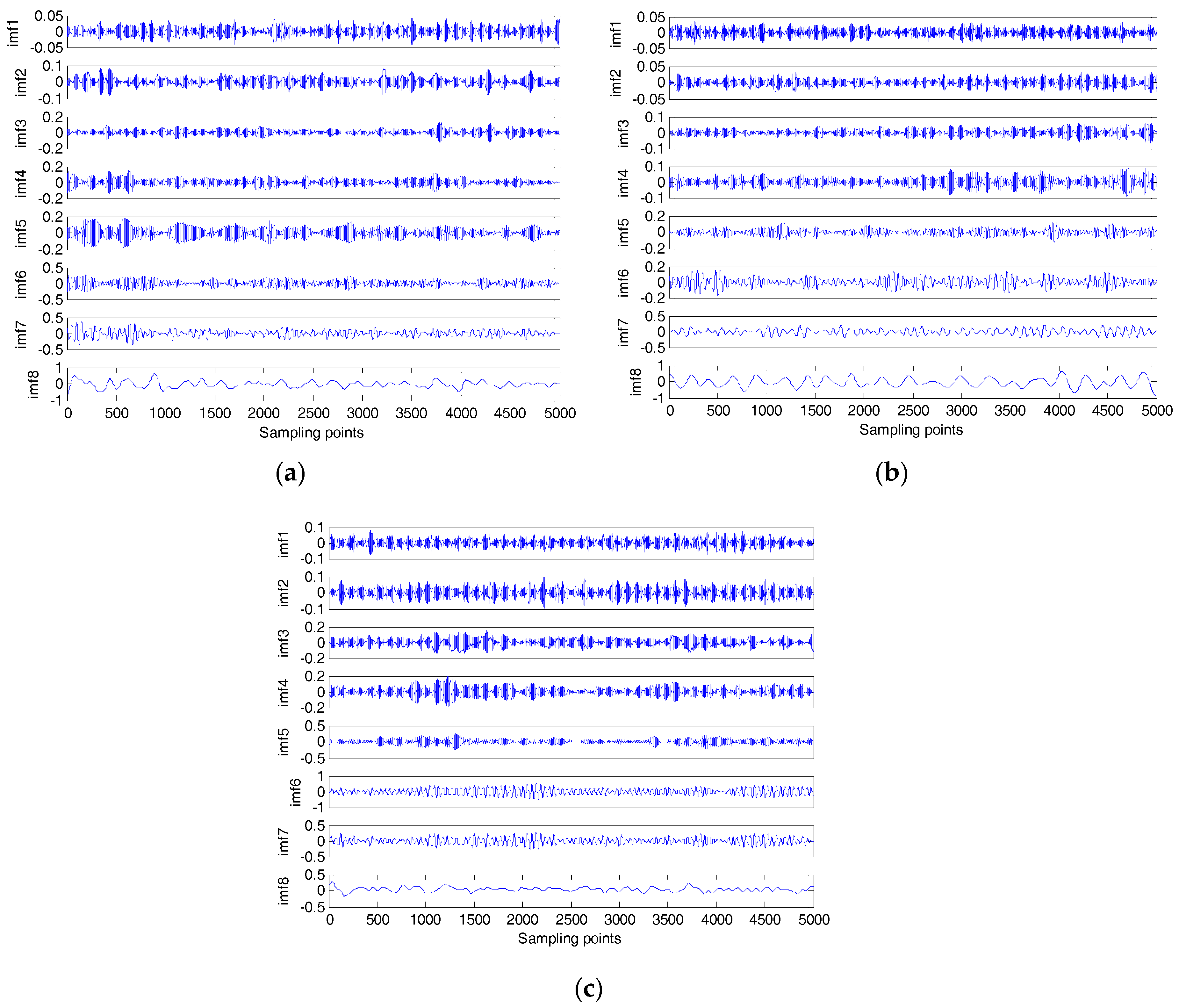
Three types of ship-radiated noise signals were recorded using calibrated omnidirectional hydrophones at a depth of 29 m in the South China Sea. During recording, there were no observed disturbances from biological or man-made sources. The distance between the ship and hydrophone is about 1 km. The sampling frequency and sampling points are set as 44.1 kHz and 5000, respectively. The samples are normalized to obtain the time-domain waveform for three types of ship-radiated noise signals shown in Figure 5. The number of decomposition and penalty parameter are set as 8 and 2000, respectively. Then the three samples after normalization are decomposed into IMFs by VMD, and the results of VMD are rearranged according to their frequency descending order in Figure 6.
5.2. Feature Extraction of Ship-Radiated Noise
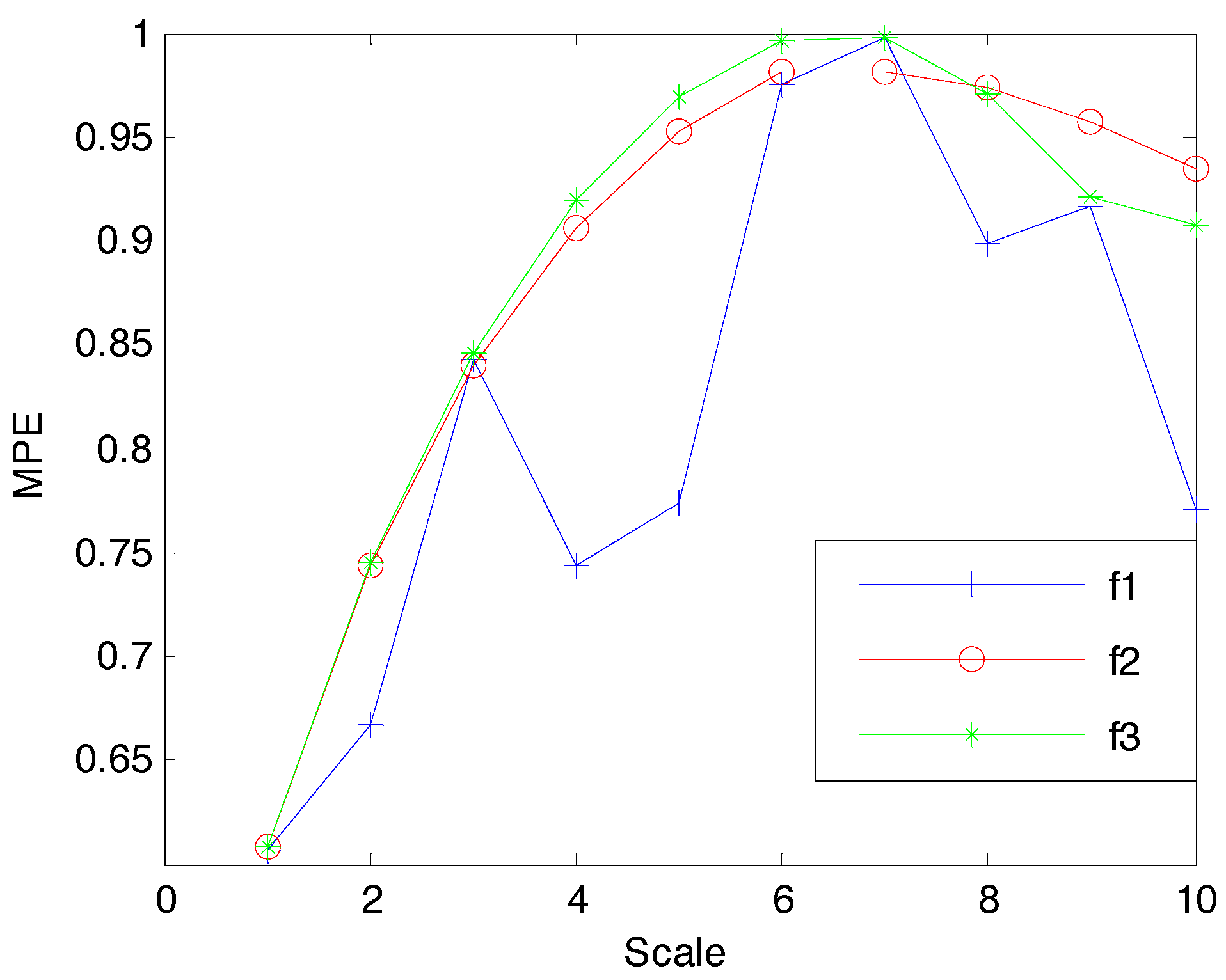
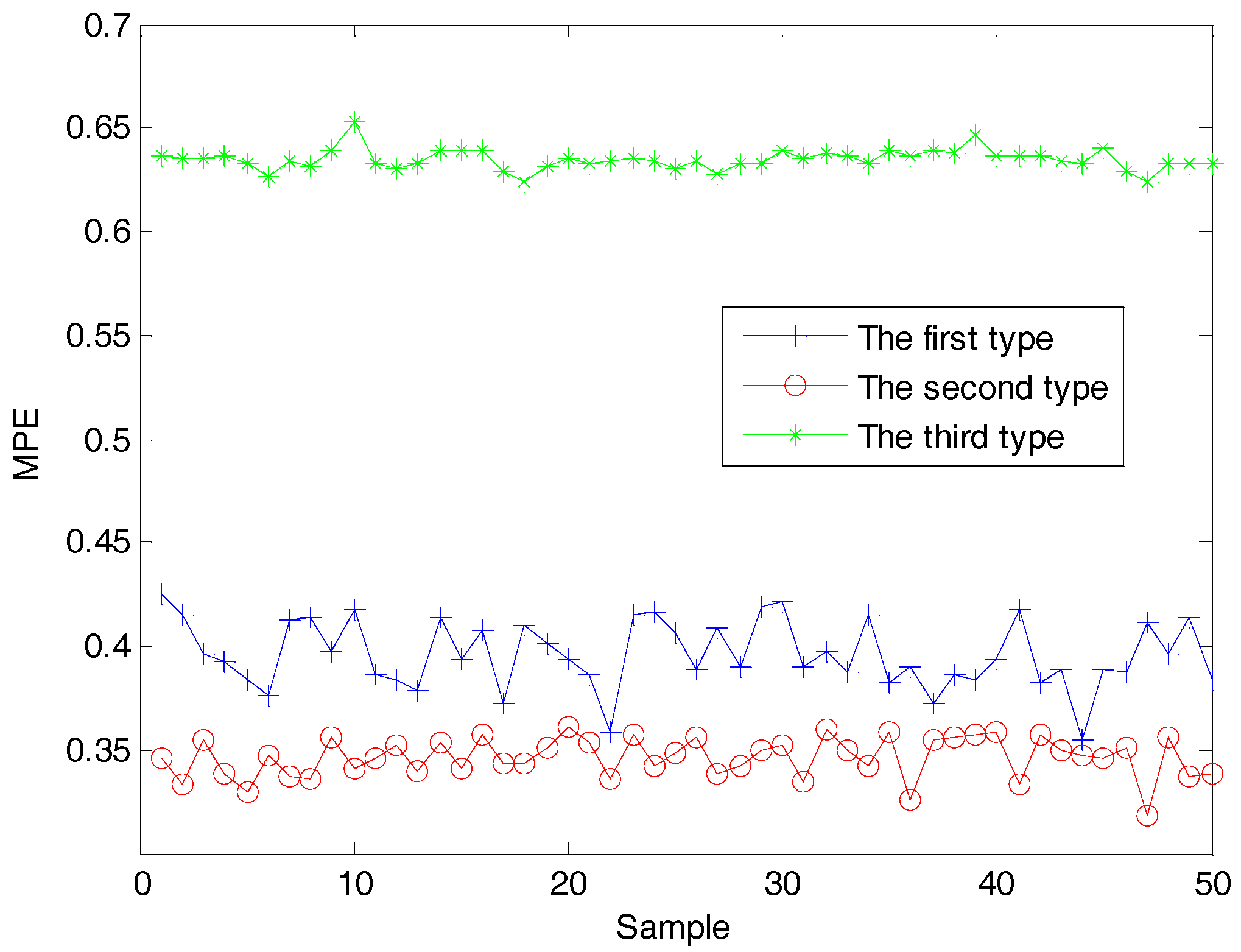
According to the VMD results, it was easy to obtain the IMF with the highest energy. The distribution of IMF with the highest energy by VMD is shown in Table 4. As shown in the Table 4, the first and second types are in the same level among them. According to the parameter settings of PE in [31], we select 4 as the embedding dimension and 1 as the time delay, the MPE of IMF with the highest energy by VMD is shown in Figure 7. As shown in the Figure 7, the MPE of IMF with the highest energy increases with the increases of scale, and the difference of MPE also increases with the increases of scale. Therefore, the MPE of IMF with the highest energy, when the scale is 5, is selected as the characteristic vector for the three types of ship-radiated noise.
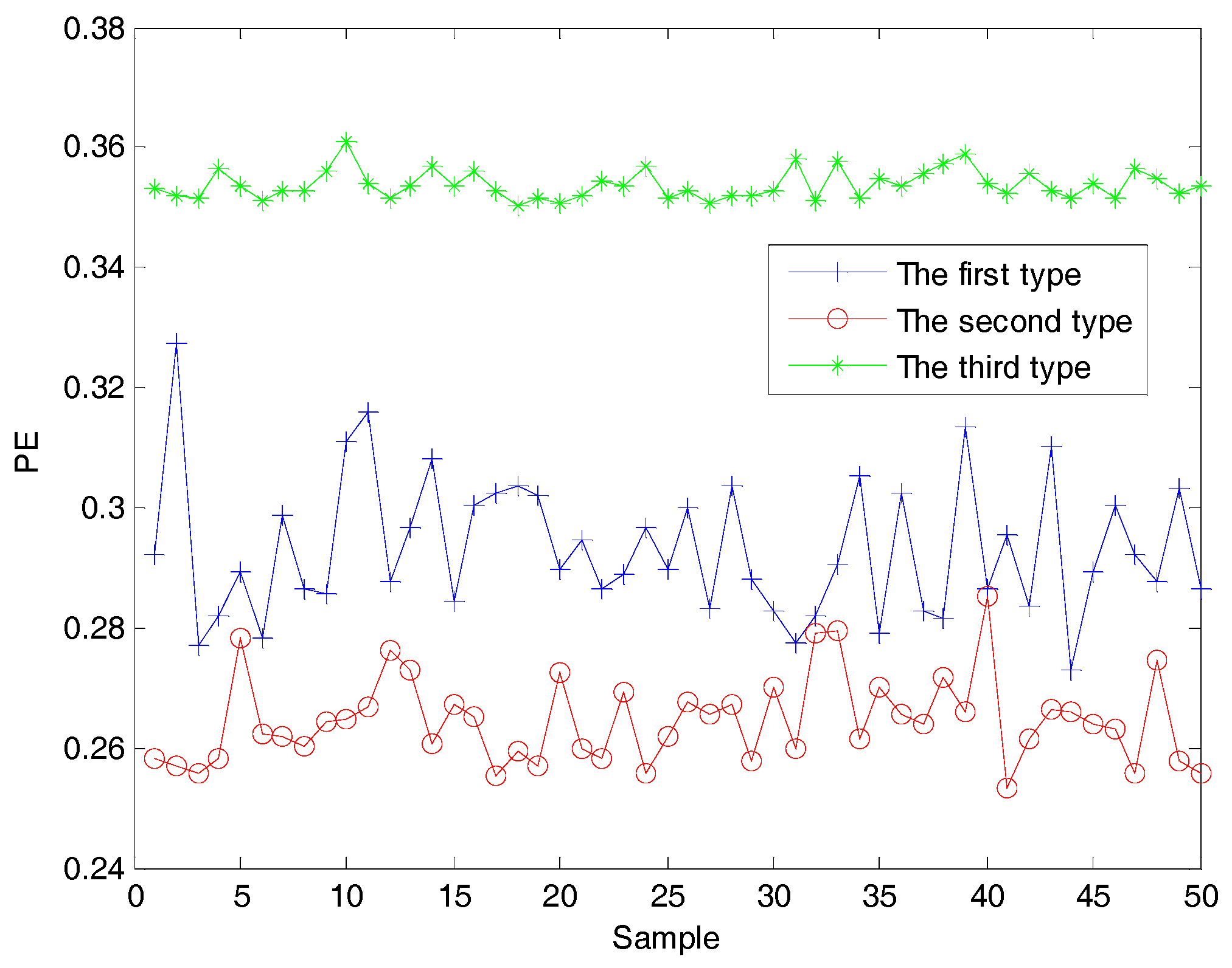
In order to prove the validity of the characteristic vector, 50 samples for each type of ship-radiated noise signals are randomly selected to calculate the characteristic vector by VMD. The PE distribution of three types of ship-radiated noise is shown in Figure 8. As shown in Figure 8, due to the presence of ocean background noise, the PE of the original three types of ship-radiated noise is greater than the PE of IMF, making it difficult to distinguish the three types of ship-radiated noise. For comparison, PEs of IMFs with the highest energy are also calculated by EMD, EEMD, and VMD, respectively. Figure 9, Figure 10 and Figure 11 are the PE distribution of IMF with the highest energy by EMD, EEMD, and VMD, and Figure 12 is the MPE distribution of IMF with the highest energy by VMD (scale = 5). As shown in the Figure 9, Figure 10, Figure 11 and Figure 12, the third type of ship-radiated noise is easy to distinguish by the four methods, however, for the first and second type of ship-radiated noise, the separability is different. The PE of IMF with the highest energy by EMD and EEMD cannot distinguish the first and second types of ship-radiated noise. The PE and MPE of IMF with the highest energy by VMD have better separability than by EMD and EEMD.
5.3. Classification of Ship-Radiated Noise
In order to further prove the effectiveness of the proposed method, the PE and MPE of IMF with the highest energy by VMD are sent into the SVM to train the SVM model and then obtain the SVM classifier. The classification results of the training sample and test sample by different methods are shown in Table 5 and Table 6. As shown in the Table 5 and Table 6, the correctness of the second and third type is 100%. However, for the first type of ship-radiated noise, the correctness is different, the correctness of the proposed method is more than 80% and the other method is less than 50%. The overall correctness of the proposed method is 94%, which is obviously superior to the other method.
6. Conclusions
To extract the characteristic vector of ship-radiated noise signals, a novel feature extraction method is proposed in the paper. The proposed method integrates VMD, MPE, and SVM. The VMD method is used to decompose the three types of ship-radiated noise signals, and the IMFs with the highest energy are obtained. Then, the MPEs of IMF with the highest energy are calculated at different scales. The optimal MPE is selected as the feature vector, which is sent into SVM to identify different types of ship-radiated noise. The effectiveness of the proposed method is fully evaluated by experiments and comparative studies. The proposed method mainly has the following advantages:
(1) Compared with [31], the proposed method uses VMD instead of EMD. Simulation results show that the VMD method is more accurate and effective than EMD and EEMD methods. The VMD method, which can effectively avoid mode mixing, is beneficial to the feature extraction of IMF.
(2) Compared with [31], the proposed method uses MPE instead of PE. PE can quantify the complexity only in one scale, while the MPE is used to extract features in different scales. The MPE can provide an optimal feature to distinguish different types of ship-radiated noise signal.
(3) By taking advantages of the VMD and MPE, the proposed method is an effective method for feature extraction of ship-radiated noise. Compared with the PE of IMF with the highest energy by EMD, EEMD, and VMD, the simulation results show that the proposed method has better separability and a higher recognition rate.
Acknowledgments
This work has been partially supported by NSFC (Natural Science Foundation of China), the fund numbers are 51179157, 51409214, and 11574250, respectively. The authors also gratefully acknowledge the helpful comments and suggestions of the reviewers, which have improved this paper.
Author Contributions
Yuxing Li and Yaan Li conceived and designed the research, Yuxing Li analysed the data and wrote the manuscript, Xiao Chen and Jing Yu collected the data. All authors have read and approved the final manuscript.
Conflicts of Interest
The authors declare no conflict of interest.
References
- Siddagangaiah, S.; Li, Y.A.; Guo, X.J.; Yang, K.D. On the dynamics of ocean ambient noise: Two decades later. Chaos 2015, 25, 103117. [Google Scholar] [CrossRef] [PubMed]
- Tucker, J.D.; Azimi-Sadjadi, M.R. Coherence-based underwater target detection from multiple disparate sonar platforms. IEEE J. Ocean Eng. 2011, 36, 37–51. [Google Scholar] [CrossRef]
- Wang, S.G.; Zeng, X.Y. Robust underwater noise targets classification using auditory inspired time-frequency analysis. Appl. Acoust. 2014, 78, 68–76. [Google Scholar] [CrossRef]
- Huang, N.E.; Shen, Z.; Long, S.R.; Wu, M.C.; Shih, H.H.; Zheng, Q.A.; Yen, N.; Tung, C.C.; Liu, H.H. The empirical mode decomposition and the Hilbert spectrum for nonlinear and non-stationary time series analysis. Proc. R. Soc. Lond. 1998, 454, 903–995. [Google Scholar] [CrossRef]
- Wu, Z.; Huang, N.E. A study of the characteristics of white noise using the empirical mode decomposition method. Proc. R. Soc. Lond. 2004, 460, 1597–1611. [Google Scholar] [CrossRef]
- Wu, Z.; Huang, N.E. Ensemble empirical mode decomposition: A noise-assisted data analysis method. Adv. Adapt. Data Anal. 2009, 1, 1–41. [Google Scholar] [CrossRef]
- Dragomiretskiy, K.; Zosso, D. Variational mode decomposition. IEEE Trans. Signal Process. 2014, 62, 531–544. [Google Scholar] [CrossRef]
- Wang, Y.X.; Liu, F.Y.; Jiang, Z.S.; He, S.L.; Mo, Q.Y. Complex variational mode decomposition for signal processing applications. Mech. Syst. Signal Process. 2017, 86, 75–85. [Google Scholar] [CrossRef]
- Lei, Y.; He, Z.; Zi, Y. Application of the EEMD method to rotor fault diagnosis of rotating machinery. Mech. Syst. Signal Process. 2009, 23, 1327–1338. [Google Scholar] [CrossRef]
- Wang, Y.X.; Markert, R.; Xiang, J.W.; Zheng, W.G. Research on variational mode decomposition and its application in detecting rub-impact fault of the rotor system. Mech. Syst. Signal Process. 2015, 60–61, 243–251. [Google Scholar] [CrossRef]
- Shih, M.T.; Doctor, F.; Fan, S.Z.; Jen, K.K.; Shieh, J.S. Instantaneous 3D EEG Signal Analysis Based on Empirical Mode Decomposition and the Hilbert-Huang Transform Applied to Depth of Anaesthesia. Entropy 2015, 17, 928–949. [Google Scholar] [CrossRef]
- Xie, P; Yang, F.; Li, X. Functional coupling analyses of electroencephalogram and electromyogram based on variational mode decomposition-transfer entropy. Acta Phys. Sin. 2016, 65, 118701. [Google Scholar]
- Xue, C.F.; Hou, W.; Zhao, J.H.; Wang, S.G. The application of ensemble empirical mode decomposition method in multiscale analysis of region precipitation and its response to the climate change. Acta Phys. Sin. 2013, 62, 109203. [Google Scholar]
- Yang, L. An empirical mode decomposition approach to feature extraction of ship-radiated noise. In Proceedings of the 4th IEEE Conference on Industrial Electronics and Applications, Xi’an, China, 25–27 May 2009; pp. 3682–3686. [Google Scholar]
- Yang, H.; Li, Y.; Li, G. Energy analysis of ship-radiated noise based on ensemble empirical mode decomposition. J. Vib. Shock 2015, 34, 55–59. [Google Scholar]
- Li, Y.; Li, Y.; Chen, X. Ships’ radiated noise feature extraction based on EEMD. J. Vib. Shock 2017, 36, 114–119. [Google Scholar]
- Zhang, Z.; Liu, C.; Liu, B. Ship noise spectrum analysis based on HHT. In Proceedings of the 2010 IEEE 10th International Conference on Signal Processing (ICSP), Beijing, China, 24–28 October 2010; pp. 2411–2414. [Google Scholar]
- Liu, Y.Y.; Yang, G.L.; Li, M.; Yin, H.L. Variational mode decomposition denoising combined the detrended fluctuation analysis. Signal Process. 2016, 125, 349–364. [Google Scholar] [CrossRef]
- Wang, Y.; Marker, R. Filter bank property of variational mode decomposition and its applications. Signal Process. 2016, 120, 509–521. [Google Scholar] [CrossRef]
- Zanin, M.; Zunino, L.; Rosso, O.A.; Papo, D. Permutation entropy and its main biomedical and econophysics applications: A review. Entropy 2012, 14, 1553–1577. [Google Scholar] [CrossRef]
- Wu, S.D.; Wu, P.H.; Wu, C.W.; Ding, J.J.; Wang, C.C. Bearing fault diagnosis based on multiscale permutation entropy and support vector machine. Entropy 2012, 14, 1343–1356. [Google Scholar] [CrossRef]
- Gao, Y.; Villecco, F.; Li, M.; Song, W. Multi-Scale permutation entropy based on improved LMD and HMM for rolling bearing diagnosis. Entropy 2017, 19, 176. [Google Scholar] [CrossRef]
- Sharma, R.; Pachori, R.B.; Acharya, U.R. Application of entropy measures on intrinsic mode functions for automated identification of focal electroencephalogram signals. Entropy 2015, 17, 669–691. [Google Scholar] [CrossRef]
- Tripathy, R.K.; Sharma, L.N.; Dandapat, S. Detection of shockable ventricular arrhythmia using variational mode decomposition. J. Med. Syst. 2016, 40, 1–13. [Google Scholar] [CrossRef] [PubMed]
- Shumbayawonda, E.; Fernández, A.; Hughes, M.P.; Abásolo, D. Permutation entropy for the characterisation of brain activity recorded with magnetoencephalograms in healthy ageing. Entropy 2017, 19, 141. [Google Scholar] [CrossRef]
- Hsieh, N.K.; Lin, W.; Young, H.T. High-speed spindle fault diagnosis with the empirical mode decomposition and multiscale entropy method. Entropy 2015, 17, 2170–2183. [Google Scholar] [CrossRef]
- Zhang, X.Y.; Liang, Y.T.; Zhou, J.Z.; Zang, Y. A novel bearing fault diagnosis model integrated permutation entropy, ensemble empirical mode decomposition and optimized SVM. Measurement 2015, 69, 164–179. [Google Scholar] [CrossRef]
- Tang, G.J.; Wang, X.L.; He, Y.L.; Liu, S.K. Rolling bearing fault diagnosis based on variational mode decomposition and permutation entropy. In Proceedings of the 13th International Conference on Ubiquitous Robots and Ambient Intelligence (URAI), Xi’an, China, 19–22 August 2016; pp. 626–631. [Google Scholar]
- Cheng, G.; Chen, X.H.; Li, P.; Liu, H.G. Study on planetary gear fault diagnosis based on entropy feature fusion of ensemble empirical mode decomposition. Measurement 2016, 91, 140–154. [Google Scholar] [CrossRef]
- Villecco, F.; Pellegrino, A. Entropic measure of epistemic uncertainties in multibody system models by axiomatic design. Entropy 2017, 19, 291. [Google Scholar] [CrossRef]
- Li, Y.X.; Li, Y.A.; Chen, Z.; Chen, X. Feature extraction of ship-radiated noise based on permutation entropy of the intrinsic mode function with the highest energy. Entropy 2016, 18, 393. [Google Scholar] [CrossRef]
Figure 1.
The simulation signals and the decomposition result of EMD, EEMD, and VMD. (a) Simulation signals; (b) EMD result; (c) EEMD result; and (d) VMD result.
Figure 1.
The simulation signals and the decomposition result of EMD, EEMD, and VMD. (a) Simulation signals; (b) EMD result; (c) EEMD result; and (d) VMD result.
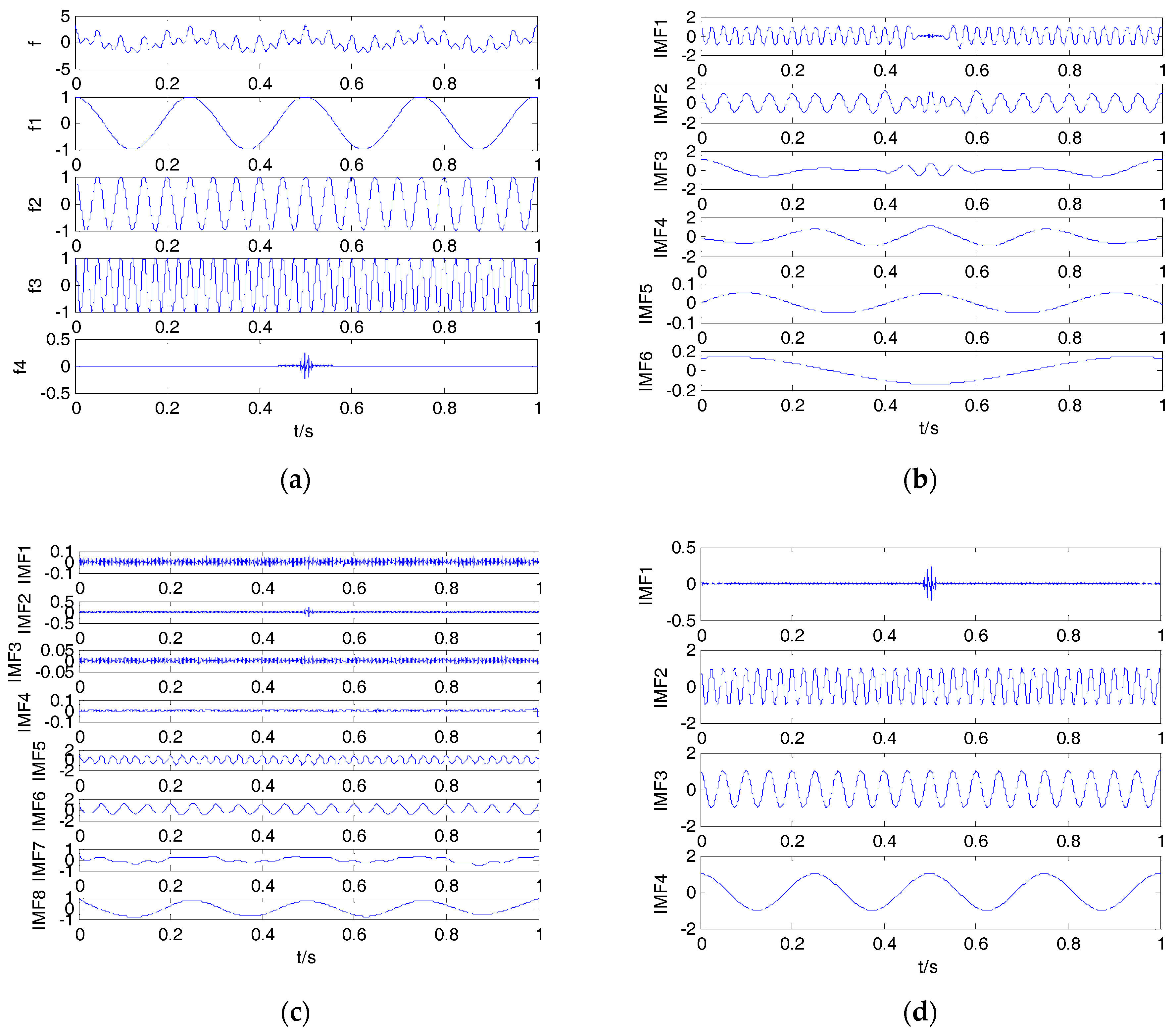
Figure 2.
The MPE of the simulation signals.

Figure 3.
The flowchart of proposed feature extraction method.
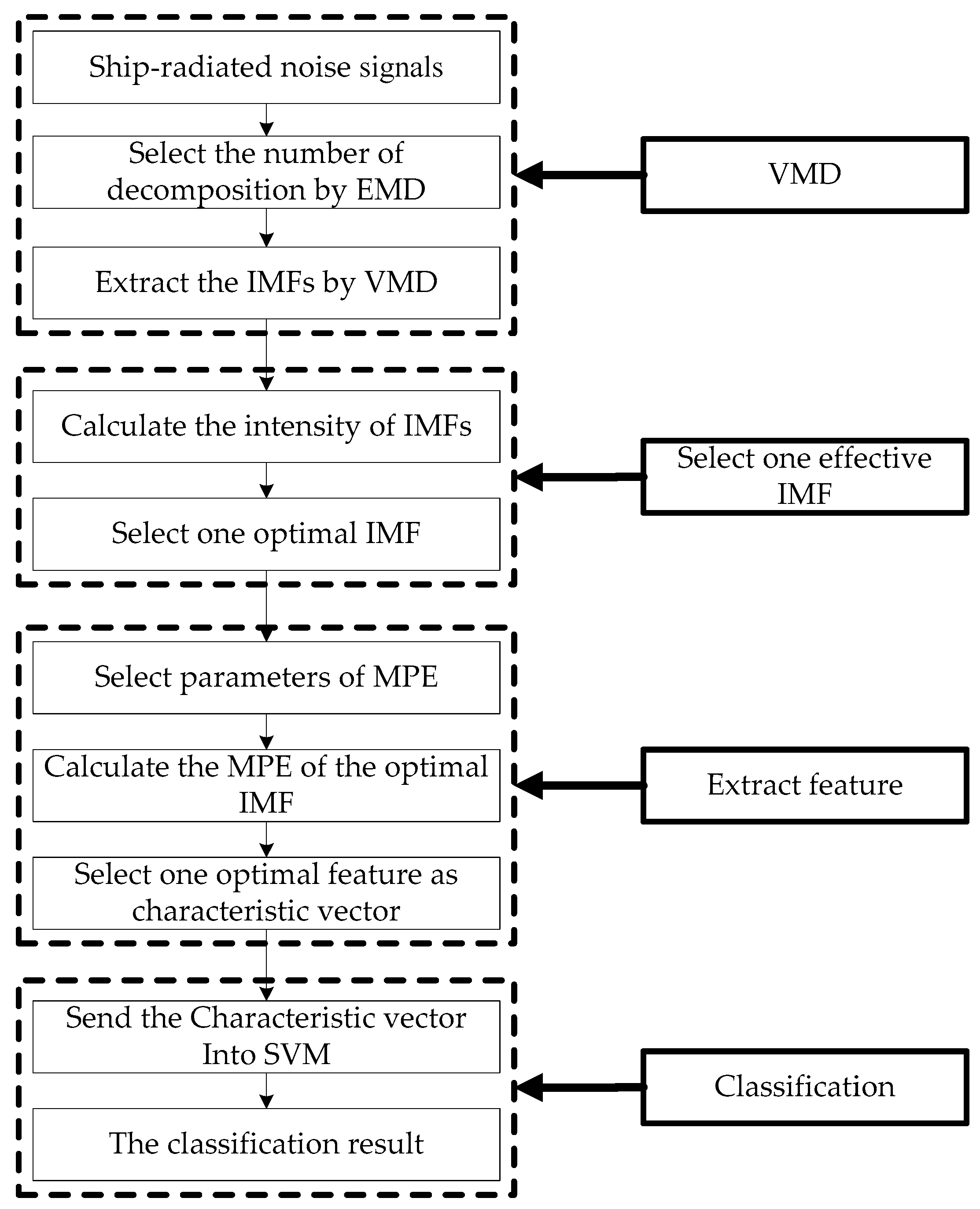
Figure 4.
The simulation signals and the decomposition result of EMD, EEMD, and VMD. (a) Simulation signals; (b) EMD result; (c) EEMD result; and (d) VMD result.
Figure 4.
The simulation signals and the decomposition result of EMD, EEMD, and VMD. (a) Simulation signals; (b) EMD result; (c) EEMD result; and (d) VMD result.
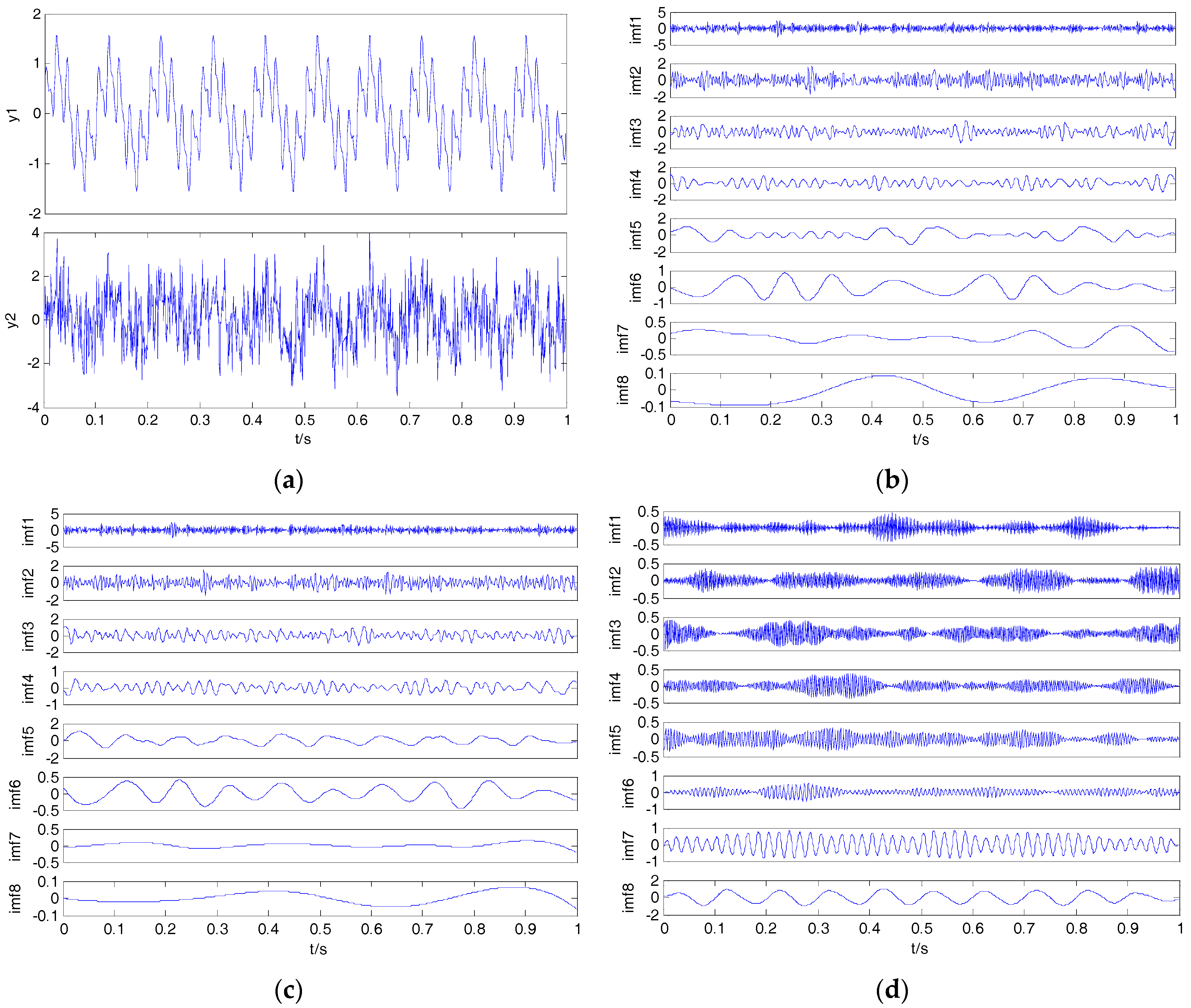
Figure 5.
The time-domain waveform for three types of ship-radiated noise. (a) The first type of ship-radiated noise; (b) the second type of ship-radiated noise; and (c) the third type of ship-radiated noise.
Figure 5.
The time-domain waveform for three types of ship-radiated noise. (a) The first type of ship-radiated noise; (b) the second type of ship-radiated noise; and (c) the third type of ship-radiated noise.

Figure 6.
The results of VMD for three types of ship-radiated noise. (a) The first type of ship-radiated noise; (b) the second type of ship-radiated noise; and (c) the third type of ship-radiated noise.
Figure 6.
The results of VMD for three types of ship-radiated noise. (a) The first type of ship-radiated noise; (b) the second type of ship-radiated noise; and (c) the third type of ship-radiated noise.

Figure 7.
The MPE of IMF with the highest energy by VMD.
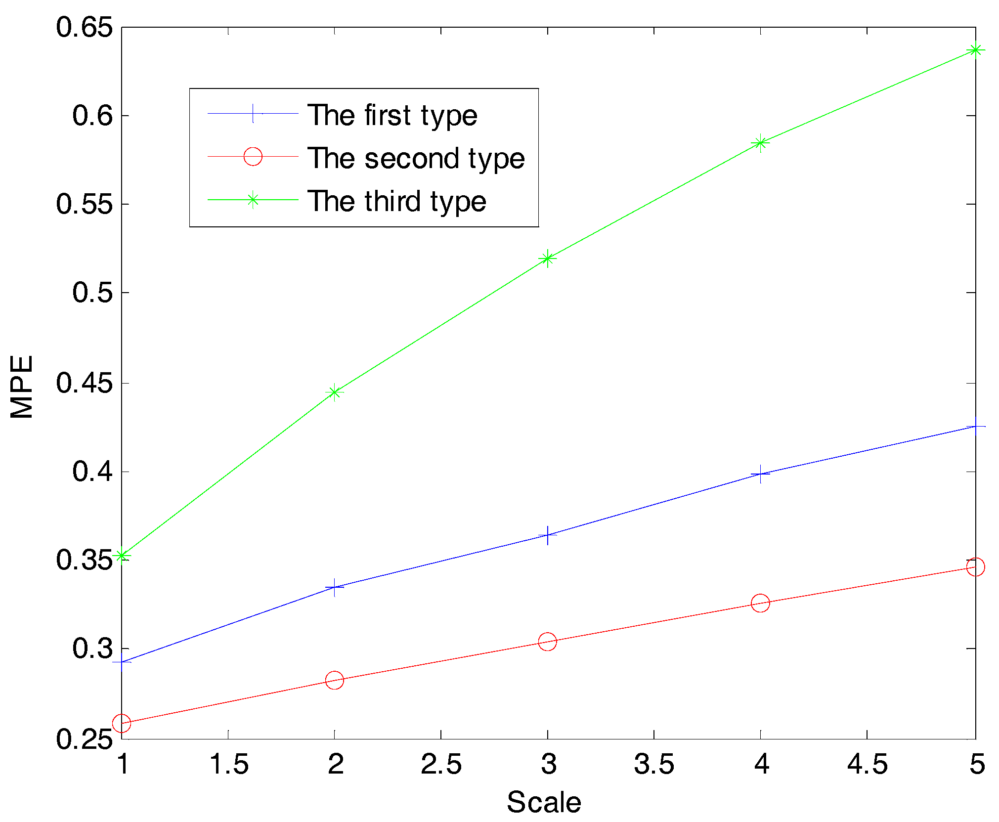
Figure 8.
The PE distribution of three types of ship-radiated noise.

Figure 9.
The PE distribution of IMF with the highest energy by EMD.
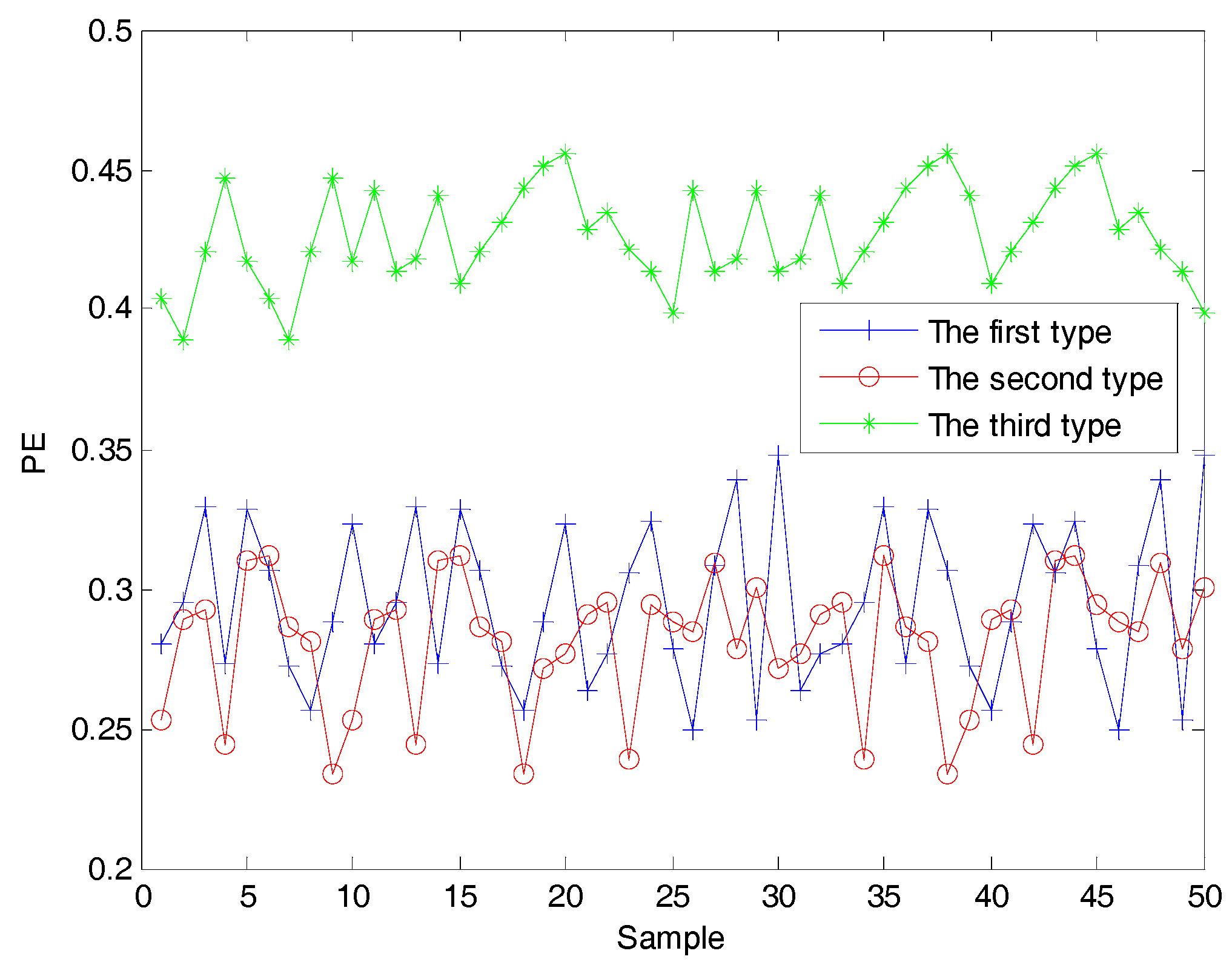
Figure 10.
The PE distribution of IMF with the highest energy by EEMD.
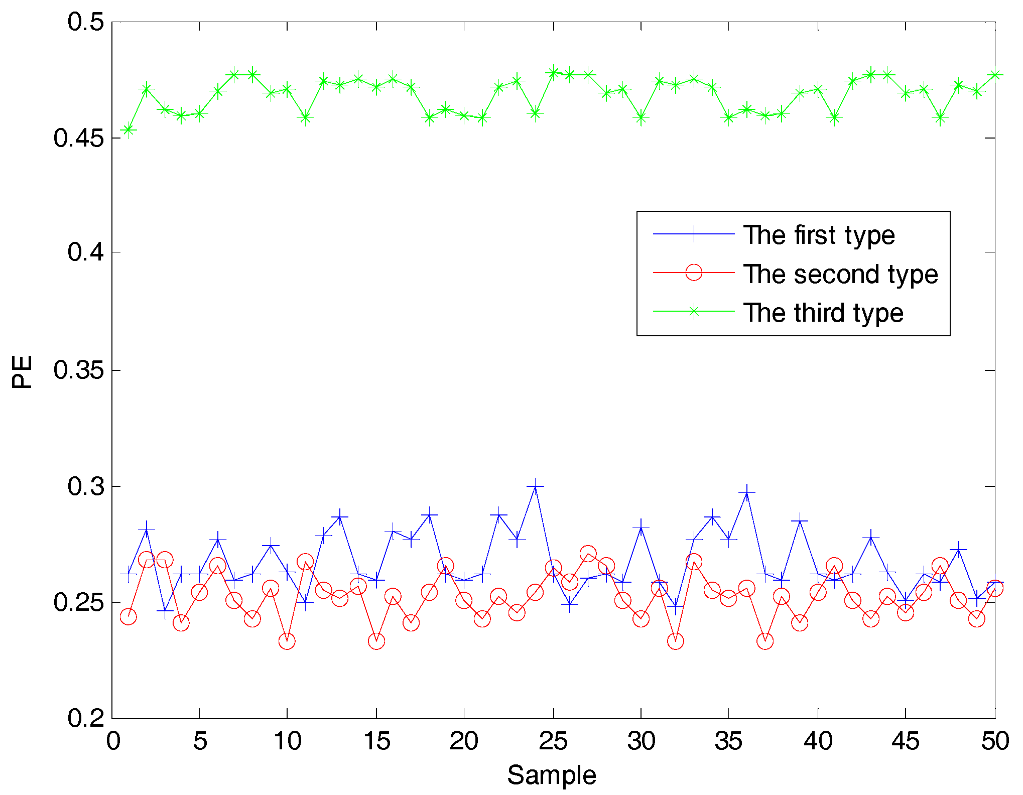
Figure 11.
The PE distribution of IMF with the highest energy by VMD.

Figure 12.
The MPE distribution of IMF with the highest energy by VMD (scale = 5).


Table 1.
The correlation coefficients of simulation signals and corresponding IMFs.
| EMD | EEMD | VMD | ||||
|---|---|---|---|---|---|---|
| — | — | IMF2 | 0.8947 | IMF1 | 0.9833 | |
| IMF1 | 0.9538 | IMF5 | 0.9928 | IMF2 | 1 | |
| IMF2 | 0.9188 | IMF6 | 0.9731 | IMF3 | 1 | |
| IMF4 | 0.8274 | IMF8 | 0.9664 | IMF4 | 1 | |
Table 2.
The IMFs corresponding to the simulation signals.
| EMD | EEMD | VMD | |
|---|---|---|---|
| S1 | IMF5 | IMF5 | IMF8 |
| S2 | IMF4 | IMF4 | IMF7 |
| S3 | IMF3 | IMF3 | IMF6 |
Table 3.
The MPE of IMF with the highest energy by different decomposition methods.
| S1 | EMD | EEMD | VMD | |
|---|---|---|---|---|
| MPE (scale = 1) | 0.4478 | 0.4869 | 0.4578 | 0.4504 |
| MPE (scale = 2) | 0.4809 | 0.5584 | 0.5122 | 0.4947 |
Table 4.
The distribution of IMF with the highest energy by VMD
| The First Type | The Second Type | The Third Type | |
|---|---|---|---|
| IMF(level) | 8 | 8 | 6 |
Table 5.
The PE classification results by VMD.
| Types of Ships | Train Sample | Test Sample | Overall Correctness (%) | ||
|---|---|---|---|---|---|
| Number | Correctness (%) | Number | Correctness (%) | ||
| First type | 20 | 45 | 30 | 30 | 78.67 |
| Second type | 20 | 100 | 30 | 100 | |
| Third type | 20 | 100 | 30 | 100 | |
Table 6.
The MPE classification results by VMD (scale = 5).
| Types of Ships | Train Sample | Test Sample | Overall Correctness (%) | ||
|---|---|---|---|---|---|
| Number | Correctness (%) | Number | Correctness (%) | ||
| First type | 20 | 80 | 30 | 83.33 | 94 |
| Second type | 20 | 100 | 30 | 100 | |
| Third type | 20 | 100 | 30 | 100 | |
© 2017 by the authors. Licensee MDPI, Basel, Switzerland. This article is an open access article distributed under the terms and conditions of the Creative Commons Attribution (CC BY) license (http://creativecommons.org/licenses/by/4.0/).
Share and Cite
MDPI and ACS Style
Li, Y.; Li, Y.; Chen, X.; Yu, J. A Novel Feature Extraction Method for Ship-Radiated Noise Based on Variational Mode Decomposition and Multi-Scale Permutation Entropy. Entropy 2017, 19, 342. https://doi.org/10.3390/e19070342
AMA Style
Li Y, Li Y, Chen X, Yu J. A Novel Feature Extraction Method for Ship-Radiated Noise Based on Variational Mode Decomposition and Multi-Scale Permutation Entropy. Entropy. 2017; 19(7):342. https://doi.org/10.3390/e19070342
Chicago/Turabian StyleLi, Yuxing, Yaan Li, Xiao Chen, and Jing Yu. 2017. "A Novel Feature Extraction Method for Ship-Radiated Noise Based on Variational Mode Decomposition and Multi-Scale Permutation Entropy" Entropy 19, no. 7: 342. https://doi.org/10.3390/e19070342
Note that from the first issue of 2016, this journal uses article numbers instead of page numbers. See further details here.