Program for the Special State Theory of Quantum Measurement

Physics Department, Clarkson University, Potsdam, NY 13699-5820, USA
Entropy 2017, 19(7), 343; https://doi.org/10.3390/e19070343
Submission received: 1 May 2017
/
Revised: 26 June 2017
/
Accepted: 5 July 2017
/
Published: 8 July 2017
(This article belongs to the Special Issue Foundations of Quantum Mechanics)
Abstract
:Establishing (or falsifying) the special state theory of quantum measurement is a program with both theoretical and experimental directions. The special state theory has only pure unitary time evolution, like the many worlds interpretation, but only has one world. How this can be accomplished requires both “special states” and significant modification of the usual assumptions about the arrow of time. All this is reviewed below. Experimentally, proposals for tests already exist and the problems are first the practical one of doing the experiment and second the suggesting of other experiments. On the theoretical level, many problems remain and among them are the impact of particle statistics on the availability of special states, finding a way to estimate their abundance and the possibility of using a computer for this purpose. Regarding the arrow of time, there is an early proposal of J. A. Wheeler that may be implementable with implications for cosmology.
1. Introduction
The interpretation of the quantum measurement process has been a puzzle for about a century now. For most applications, the puzzle can be ignored. However, when one deals with the interface of the macroscopic and microscopic—and, in particular, when a microscopic system is “measured” and the information is passed to a macroscopic observer (human or not)—there still rage disputes.
Perhaps a personal remark will not be out of place: proposing a solution to such a long-standing puzzle requires, as Bohr said [1], “a sufficiently crazy theory.” And there has been no shortage. I will not review the various solutions, but I do claim, as you may agree after reading this theory, that what is presented below satisfies Bohr’s criterion. In fact, I myself have trouble believing these ideas, but what motivates me is that the alternatives are even more difficult to accept [2,3].
In Section 2 is a review of the entire theory with the first subsection devoted to quantum aspects (Section 2.1). Following that (Section 2.2) I discuss the way in which there is a departure from the usual arrow of time. In a final review, Section 2.3, I deal with recovery of the Born probabilities.
Once the theory is reviewed, I discuss the numerous open problems. First, there is the matter of an experimental test. In my book [4], in-principle tests were proposed, but they did not seem practical. However, more recently, do-able experiments have been formulated [5,6,7] and this will be discussed here. Then, there are theoretical problems. Although the recovery of probabilities might attain a level of mathematical elegance, it is in fact an avoidance of contradiction, rather than a positive demonstration. There is also the matter of the abundance of special states. One aspect that demands investigation is the influence of particle statistics on abundance. Then, there is the matter of overall abundance itself. I will argue that the need for definite measurements (and thus special states) is ubiquitous, not only in formal measurements, but in essentially all macroscopic interactions. Can there be enough special states for this?
As indicated by the title of this article, it is an outline of a program. Most of the questions just posed await answers. My feeling has been that the experimental test is the primary issue—given a positive result, theory will follow.
Finally, I remark on the fact that there is an experimental test. This means that the theory to be advanced is not an interpretation, not a hidden variable theory. It has well-defined predictions and outcomes that differ from those predicted by either the Copenhagen interpretation or the Many Worlds interpretation (MWI) and their many variants.
2. Theory Review
In the following subsections, I give a brief review of the special state theory of quantum measurement. In this theory, measurement is not a deviation from the usual quantum mechanics: it is just unitary time evolution. I remark that, since the early days of quantum mechanics, experimental technique has blurred the line between macro and micro, and there has never been any indication of any dynamics but unitary time evolution. The special state theory thus shares a common view with the Many Worlds interpretation. The difference is that I have only one world. This requires significant modification of statistical mechanics, as well as the existence of particular quantum states, states that I call special. I begin with the quantum aspects.
2.1. Special States in Quantum Mechanics
To see how special states operate, I consider an example.
Suppose there is a single 2-state system in contact with a heat bath of bosons [8]. Initially, the system is in its excited state (spin-up) and the boson coupling induces the decay. This model of measurement misses much of the real world, like “registering” the measurement, i.e., making sure the system does not return to its excited state (irreversibility). These features are assumed to result from parts of the system that I do not model [9]. I use the spin boson model with a single boson, for which I can take the Hamiltonian [10] to be
The Pauli spin matrices are the operators for the 2-state (spin) system, a and are the boson operators and , and are parameters.
As indicated, the single spin starts (say) as , and the coupling to the bath tends to flip it over. The special states are particular initial conditions of the bath such that the microscopic final state of the spin is (either) all up or all down (i.e., or for real ). “Final” in this case refers to a specific time, namely that time at which a large, irreversible system notes the state of the spin. Such “special” states would be rare, since, after any reasonable amount of time, the microscopic state would be partly up, partly down, something of the form for nonzero and .
Let us be specific. The system has Hamiltonian (1) with , , and . The spin starts in , with the oscillator state unspecified. The finiteness of the computer requires that the oscillator be cut off, and I only considered 250 states. (This led to an error in in the diagonal term, but not elsewhere. To reduce the effect of this, only states with relatively small probability in the highest levels were considered.) For these parameters at time-0.15 (which is the specific time, the time at which a large irreversible “observer” [11] looks at the spin), there is about a 50% probability of decay, namely if one would trace out over the oscillator states, the density matrix for the spin would be half-half.
However, it is not the average that concerns us here. It’s the issue of whether there are any states that have either entirely decayed, or not decayed at all. The way to learn this [4] is to define a projection operator [12] on the spin: . Using this operator, the probability of being all up at time t is
with and where I have used . Defining and using , I have . Defining , it follows [13] that the issue of whether any initial state (of the bath) can lead to a measurement of up, using purely unitary time evolution becomes the issue of whether B has eigenvalues equal to one. Similarly, the issue of whether there any fully decayed states requires of B that it have eigenvalue zero. (Note that B’s eigenvalues are real and in the interval .)
Indeed, there are such states. One probability distribution for each case is shown in Figure 1. The figure only indicates the magnitudes of the special states; the relative phase of each component is also fixed, but not shown in the figure. Thus, the state that at time is entirely in the up position had an initial bath state of the form , with the values of shown in Figure 1a (and the particular values of , not shown). At time-0.15 this state is undecayed despite the fact that a random or average state would be a superposition of both decayed and undecayed states, with the trace (over bath states) giving about 1/2 for each eventuality. Similarly, the state whose probabilities are shown in Figure 1b has decayed almost completely at this time. (In fact, there is a slight residual probability both for decay and non-decay. In the illustration, the for the “non-decay” state is about , while of the “decay” state . This issue will be discussed near the end of Section 2.2.)
What good are these states? They constitute the main idea for avoiding many worlds while holding on to unitary time evolution.
Suppose a cat (à la Schrödinger) is placed in a chamber with the usual vial of poison. Let the dispersal of the poison be governed by the spin state just discussed. The spin-cum-bath system is also in the chamber and the entire setup isolated. Its isolation ceases at time-0.15 and the irreversible “registration” is due to the observer, who looks to see if the cat is dead or alive. (It is important to realize that with the observer included the Hilbert space of interest grows enormously [14] and the Hamiltonian Equation (1) no longer describes all of the spin’s interaction with the (now larger) world. It is in the enlarged Hilbert space that the measurement is irreversible and “registered.”) The usual problem is that there can be significant probability for both options. However, there is no problem if the initial state of the bath is one of the “special” states I have been describing. For the non-decay state, there is a living cat; for the decay state, it is dead. This is accomplished with no black magic; it is the result of unitary time evolution from the specified initial conditions.
This is the main idea of the special state theory: no macroscopic superpositions because of particular initial conditions. I mention also that there is no entanglement. At time-0.15 the spin state is wholly in one state or the other and a trace over the other coordinates would leave the oscillator state unchanged.
The next—obvious—question is: why should Nature arrange to have a “special” state as the initial conditions for every situation where a potential split into many worlds occurs? Moreover, “’final” states for one potential but avoided macroscopic superposition are initial conditions for the next. Thus, this implies both an extreme form of determinism and a sufficient abundance of special states. I don’t have justification for these assumptions, except to say that this is the conclusion I am driven to by insisting that no magic dynamics occurs in the measurement process and that there is only one world. What I can offer though is perspective. How strange is it for there to be particular, non-random, initial conditions? For this, I turn to the next subsection.
2.2. Thermodynamics and the Arrow of Time
As discussed in [4], the usual arrow of time is equivalent to using random initial conditions. However, this assumption has never been verified experimentally; its main virtue is that answers arrived at based on this agree with experiment—not to be sneered at, but not a proof.
I will use a simple model of mixing dynamics to show that the assumption of random initial conditions is unnecessary. The model is the cat map [15], a transformation of the unit square (with coordinates ) into itself
Imagine an ideal gas of N such points in the unit square, each moving in discrete time under the cat map. For example, in Figure 2, I show the behavior of a collection of points initially satisfying and . This system is headed for chaos. A quantitative measure of this “chaos” is the information entropy, where it assumed that perfect knowledge of the state is not available to the evaluator of the entropy. This imprecision is expressed by a coarse graining of the x-y coordinates. For example, one can imagine that only the first decimal place of a point’s location is known, i.e., the grains are the 100 1/10 by 1/10 squares contained in the unit square. The entropy is then calculated by counting the number of points in each grain. With this coarse graining, the entropy is
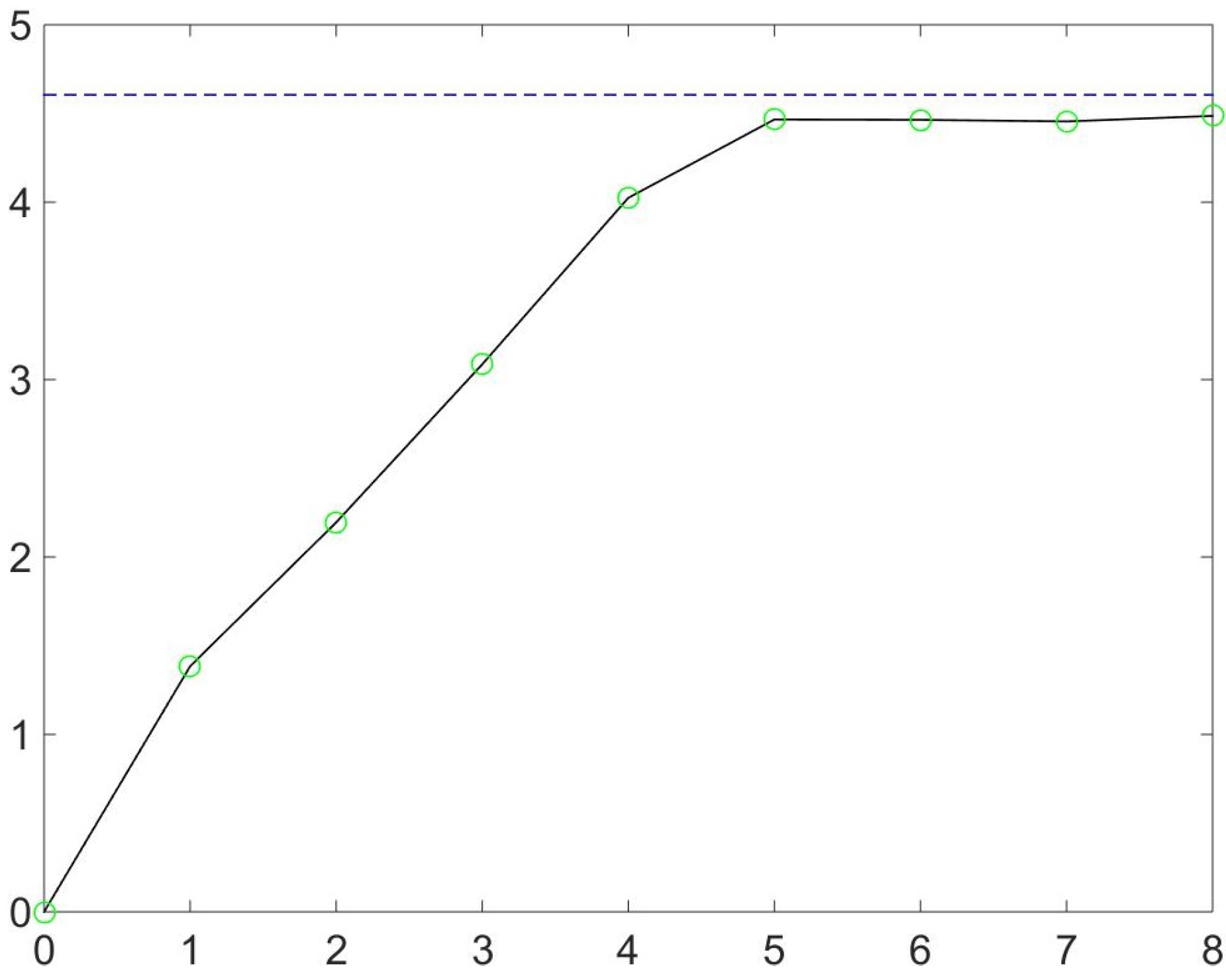
where k labels the coarse grain and is the number of points in the grain. The time dependence of the entropy for the evolution in Figure 2 is shown in Figure 3.
This is a manifestation of the normal arrow of time: the initial points were selected randomly within a particular grain and the entropy increases monotonically until close to equilibrium, after which it fluctuates below that value.
However, consider a simulation for which the initial points were not selected randomly, although for the first few time steps, it will look that way. The simulation runs 18 time steps from the initial square and is shown in Figure 4. The images should be read left-to-right and row-by-row. There are 4000 points and most time steps are shown. Note that every point in this simulation evolves by pure cat map dynamics. So how did I get these images? It was easy. I randomly occupied the first little square ( and ) at time-0 with about 120,000 () points. Then, I imposed two conditions. First, at time-18, they needed to occupy a different little square of the same size as the original. This reduced the acceptable points by a factor 25. Then, I also demanded that, at time-9, the points resembled the face of a cat. This reduced the numbers further, but I nevertheless was able to keep 4000 points that satisfied all conditions. For non-interacting points, the 3-time boundary value problem was easy to solve: removing one point did not affect the others.
The message of this demonstration is most poignant when phrased in terms of entropy. For each configuration in the sequence with the initial conditions of Figure 4, the entropy is computed (using grain sizes of 1/5 × 1/5) and is given by the circles in Figure 5. A second curve, with markers in the form of stars, is also shown. It is the entropy for 4000 points initially starting in the same coarse grain, but purely random, with no future boundary conditions. Compare the two curves. My point is that for times prior to about 7, you cannot tell the difference.
The conclusion is clear: there may be future constraints, but you would not know about it. The arrow of time does not (necessarily) point as fixedly as one might have supposed.
Alternatively, you could say that the initial points that yielded Figure 4 were not random but had a cryptic constraint. It was a difficult to discern, but as the dynamics unfolded, it dominated the images.
This example is intended to justify the idea that there could be other cryptic constraints. Not every imaginable state occurs in Nature, only those which are “special” in the sense that I use the term. This is a severe restriction, but it is one that can be invisible. The formulation of this restriction that I find most palatable is a two-time boundary condition. This contradicts the usual arrow of time, but as demonstrated, its effect need not be noticed except near the boundaries, which may be well-separated [16].
What kind of two-time boundary condition could select special states? First, consider initial conditions. As Wald [17] has pointed out, in the early universe, the entropy was low, for unknown reasons. He even has trouble defining entropy, but it is clear that the universe was “special”—his word, in this case. Let’s go one step further: assume the von Neumann entropy was also low; there was little or no entanglement. In these speculations, it is not clear what is or is not permitted to be entangled. Nowadays, we have an idea of macro and micro, but it would not apply to a primordial era. Nevertheless, we’ll assume that at some stage it became meaningful to speak of entanglement and that it was minimal.
Now imagine that our entire cosmology is roughly time symmetric. This possibility is not popular today due to the discovery of accelerated expansion. However, that phenomenon is poorly understood and there have been suggestions of a periodic cosmology despite the acceleration (a small sample is [18,19]). One additional component enters, the connection first suggested by T. Gold [20], relating the arrow of time to an expanding universe. One then expects [21] that under contraction the arrow will be reversed. Recalling the connection between boundary conditions and the arrow of time, one can now enunciate a possible boundary condition that would demand special states: little entanglement at the beginning, little entanglement at the end [22].
To see how this condition demands special states, consider a Schrödinger cat. At the end of the experiment—and again demanding only unitary time evolution—in the MWI, there is a portion of the wave function with a dead cat and a portion of the wave function having support on a macroscopic state recognized as a living cat. The dead one is buried, the living one doesn’t want more of this experimentation and disappears from the lab. However, how can these portions of the wave function be recombined coherently, as they would need to be if there is a no-entanglement demand in our future. Because they have decohered, it would take tremendous coordination to accomplish this coherently. Having a special state is also an unlikely way to avoid entanglement, but it is much less unlikely than recombining after a superposition of macroscopically distinct states has formed.
With the two-time boundary condition rationale, one can consider the small amount of leftover wave function, as seen in my special state example above. As indicated, the special state for decay has a small but non-zero probability of non-decay (in the examples, it is roughly ). In the context of a boundary value problem, one does not need perfection. The measure of possible error in “specializing” is given by the tolerance of that boundary value problem. I also expect that even this level of error is much larger than what occurs in nature and represents a limitation of my computer modeling. This will be discussed in Section 3.
Aside on cosmology and Wheeler’s idea: John A. Wheeler proposed [23] the following way to bound the big bang-big crunch time (if there would be a big crunch). Take a laboratory sample of (say) (lifetime year, not the example he gave) and check how it decays. Is it exponential or would a better fit be a hyperbolic cosine? If the decay resembled a cosh, then it would reflect a two-time boundary condition and would give an estimate of the lifetime of the universe. You didn’t even have to look out the window of your laboratory. I analyzed this idea using a simple model [24,25] and found it to be flawed, and that at the least you’d need to know the overall abundance (in the universe) of the isotope in question.
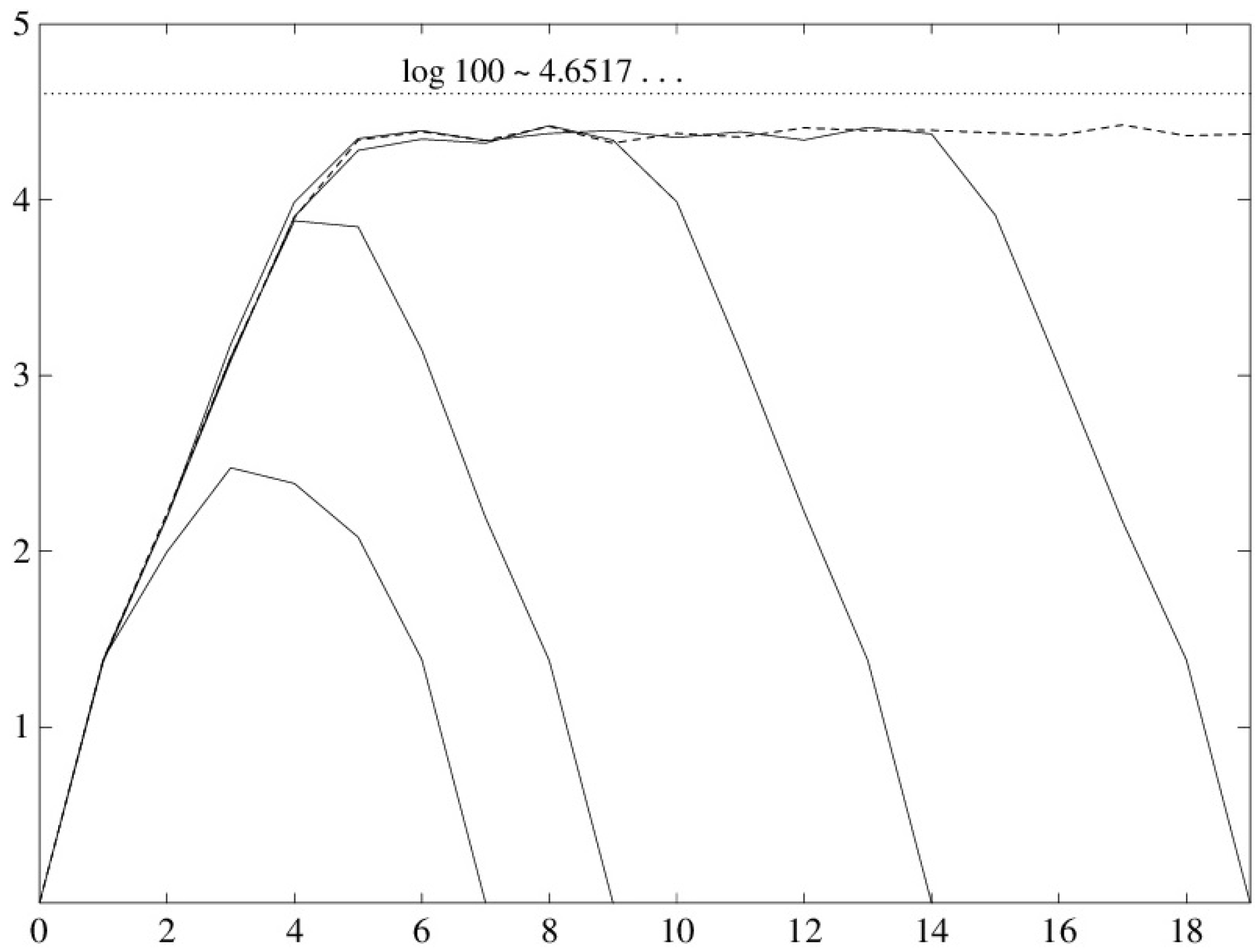
However, there was still a way to implement the idea. Find a process with relaxation time on the scale of the lifetime of the universe and see if the relaxation is normal. As you can see in Figure 6, if the relaxation time is long enough, anomalies will be evident. One such process is the formation of the galaxy distribution described by large scale structure. These days, most cosmologists favor the idea that the universe is not only going to expand forever, but that expansion will become ever more rapid. However, I have seen enough cosmological theories go out of fashion to believe that it is still worth thinking about testing this effect.
Finally, there is the issue of recovering the Born probabilities. If every experiment involves interaction with apparatus and special states, why is it that probabilities can be calculated using only the wave function of the system being studied? This is our next subject.
2.3. Recovering the Born Probabilities
In the usual interpretations of quantum mechanics, you don’t need to pay much attention to the apparatus: to calculate the probability of various outcomes, you only need the wave function of the system being measured. By contrast, the special state theory must also construct the wave function of the apparatus. It therefore seems necessary to make the following claim: the abundance of special states of the apparatus reflects the wave function of the system being measured. For example, suppose you have two outcomes to an experiment, with respective amplitudes and (so ). Then, the number of special states (whose consideration requires looking at a much larger space) for each outcome will correspond to the same relative probabilities, that is, and . Thus, although the space of special states is small compared to that of all states, nevertheless, the vector space for each outcome is still comprised of many dimensions and the relative dimensions reflect the usual probabilities. In this way, “probability” in quantum mechanics becomes like probability in classical mechanics [26]. The outcome is determined (by unitary time evolution), but since you don’t know which special state is involved, you must fall back on probabilities. This is not a hidden variable theory. The ignorance of which special state is involved reflects the macroscopic nature of the apparatus. In principle, if one knew the microscopic state, one would know the outcome with certainty.
I will come back to this claim in Section 3. For now, I will establish a much weaker result. The actual special states will not be identified, but their possible statistics will be studied. What looks at first to be impossible will turn out to require a particular structure in the abundance issue.
Consider the simplest quantum measurement problem, determining the state of a two-level system. For convenience, I study a Stern–Gerlach (SG) apparatus measuring the spin along the z-axis. Let the initial spin state be
(In this basis, up means an eigenstate of the z-component of spin with a magnitude 1 entry in the upper portion—correspondingly for down.) There are of course many other degrees of freedom in this problem. Foremost is the position of the spin (riding perhaps on a K atom); then, there is the macroscopic magnet, macroscopic screen, and much more. However, I am now working backwards and will assume that lurking in various corners of this enormous Hilbert space are special states for the various outcomes (up or down). It is the statistics of these states that I study. In particular, I will consider the abundance of different special states for different angles, , of the spin orientation. At first, it will seem that this abundance issue is impossible to satisfy, but then it will be seen to impose a particular structure on the space of all spacial states.
The first step in any assessment of the availability of special states is to seek the least unlikely way in which they could occur. Of course, they are rare, but there are different levels of rarity and I seek the kind of special state that imposes the fewest conditions on the wave function. For an SG (Stern–Gerlach) experiment, the atom must ultimately be absorbed in one or another region of the target area, but not in between (or elsewhere). This can be accomplished by combining the output wave functions after they’ve left the magnet, or by rotating the spin so there is only one wave packet that emerges from the magnet (I assume familiarity with the SG setup). Rough estimates (see [6]) suggest that recombining the spins is far less achievable than rotating the spin before it even enters the magnet. Thus, the problem becomes one of rotating the spin from its initial value () to be up or down.
We assume that’s what happens; perhaps what one takes to be a stray magnetic field provides just the right force to bring the spin to 0 or , prior to its entry into the inhomogeneous field. The function of the strong, inhomogeneous field is to make the eventual position coordinate dependent on the spin with which the atom entered that field (as usual in the SG experiment).
Let us call this apparently (but not truly) random change in a “kick.” If you imagine doing several experiments with different initial ’s, the number of kicks to one or the other special value also varies. Let be the probability of obtaining a kick of size . Of course, for any one experiment, only kicks of size (with n an integer) enter, but it is reasonable to assume that, as varies, there is some well-defined distribution, manifested in our situation as a probability. Thus, to get spin up, one must have a kick of size or, if one allows for larger kicks, for positive or negative n’s. Similarly, to get spin down, one requires a kick of size (again, with integer n). Thus the probability of spin up is . Similarly, for spin down, one adds to each summand in the argument of f. On the other hand, standard quantum mechanics, i.e., the Born rules, dictate that the ratio of down to up is . Therefore, our requirement on f (hence on g) is
(In Equation (6), in the definition of g, use has been made of f’s symmetry as well as the fact that n is a dummy variable.) There is an explicit solution to Equation (6), namely . Unfortunately, this solution is not normalizable, as a probability should be. (In fact, there is no normalizable solution to Equation (6); see Appendix B of [5].) However, for close to 0, it is possible to cut off the function and eliminate the singularity without experimental implications. A convenient cutoff makes use of the Cauchy distribution
which, for small enough a, changes Equation (6) very little. The deviations from standard probabilities are the largest for and are of order ; since a is unknown, one can only bound it, since as far as I know deviations from the standard results have not been found. The distribution does not have a second moment (it is a Lévy distribution), and this may be necessary for any function f satisfying Equation (6). In [5], Appendix B I report partial proofs, but I emphasize that for the purposes of the experimental tests described below and in [6], the Cauchy distribution is not required.
3. Program: Open Problems
There are many theoretical questions about the ideas of Section 2, but I will begin discussion of the program by mentioning experiments that can be done to confirm or deny those ideas. This is because, if an experiment were to prove positive, the theory would fall into place.
3.1. Experiments
In [4], a number of experiments were proposed, but they were more for the purpose of demonstrating that the work presented was different physics, not merely another interpretation. The experiments mentioned did not seem practical. Another possibility came up in dealing with the time it took for a quantum system to change states [27], but there too it was not clear (to me at least) how practical this proposal would be.
More recently, there have been proposed experiments that should be feasible. They would be challenging, and I have not (yet?) convinced anyone to carry them out, but I believe they are in the realm of experimental technique. I have explored both variations on the SG setup and and optical versions involving photons [5,6]. In this article, I will review the experiment involving the modified SG apparatus.
3.1.1. Force-Free Rotation?
Our context is again the SG experiment, but one that has been in a sense doubled. The system passes through two strong, inhomogeneous fields, one to orient it along a particular direction (and those not so oriented, about half of them, are removed from the experiment), and the second field to measure the spins of those prepared in this way. Actually, Stern himself undertook an experiment of this sort, but, at first, he and Phipps [28] ran into trouble because, unless the magnetic field between the magnets vanishes, the spins follow the residual field adiabatically. Later, in Stern’s laboratory, Frisch and Segrè [29] overcame this problem and the four of them published their results jointly [30]. In the analysis, Frisch and Segrè used work of Majorana [31] that confirmed that the experiment was theoretically successful. (Majorana’s analysis is analytic, but it is amusing that in, the 21 century, one could use a computer to get slightly sharper results (unpublished).)
For simplicity, assume that the two strong magnetic fields sort along perpendicular directions, so that (choosing axes) the initial wave function is the plus eigenstate of . At the end of the experiment, we’ll get up or down, i.e., eigenstates of . Does this mean some force acted to rotate the spin?
In the MWI, there is no need for any force to be applied in order to go from an eigenfunction of to an eigenfunction of . The same is true for the Copenhagen interpretation. However, in the special state theory, there is! That’s the basis for the experiment.
First, see how it works in MWI. Individual observers do have a change in their perceptions of the value of the angular momentum, and this occurs because of a change in the overall wave function, but there is no need for angular momentum non-conservation. Imagine an (already) up spin sent into this apparatus. There is no transfer of , although there is a very small transfer of linear momentum, since the atom (carrying the spin) is deflected. Similarly, a down spin induces no transfer. In equations
In these equations, is the time evolution operator and represents anything not the spin or the observer, in particular the magnets and the atom’s translational degrees of freedom. I emphasize: although there is a small transfer of linear momentum, there is no transfer of z-component of angular momentum in either case. However, now consider an initial state whose spin is not oriented along the z-axis (and ),
By the superposition principle, this yields one observer who had prepared the state at a non-trivial angle to the z-axis, but found at the end a spin pointing along that axis. The same is true of the other observer (who is the same person except for this one experience, although they may diverge subsequently in other ways). Each has seen a change in the perception of the z-component of angular momentum. On the other hand, since the wave function in Equation (9) is a superposition of the initial wave functions of Equation (8), the dynamics can be separately considered for each, and there is no transfer of z-component of angular momentum at any stage. How can this be? The (version of the) observer who saw “up” will say, ’Oh, I was on the “” component of the wave function’ (in our notation), while the other (version of the) observer would make a similar statement, with replacing .
One should not find this shocking. Despite the observer’s possible perplexity, there is conservation of angular momentum. The total Hamiltonian commutes with the (total) operator; it is just that each observer, decohered from the other, sees a peculiarity.
The explanation would be slightly different for (my understanding of) the Copenhagen interpretation. Until you actually measure , it has no value, since does not commute with the projector for the spin state in Equation (9).
However, with only one world—the contention of the special state theory—there can be no change in the wave function without a proximate cause. If a quantity is changed, the single observer can, if it is practically possible, determine what caused the change. This proximate cause lies in the special state itself. If (of the spin) changes its value, something else has to pick it up [32]. This “something” can only be due to the peculiarities of the special state, what has been called a kick earlier. (Recall, the kick is not a deviation from the laws of nature, but like the cat at time-9 in the progression of Figure 4, it is the result of exact obedience to the rules, but happening because of unusual initial conditions [33].)
As discussed, the most likely (or least unlikely) form of the kick is that a short term magnetic force acts to bring to or (up to phase factors). The first point to investigate is how large a field is needed. Unfortunately, I do not know much about the special state that does this rotating; presumably, it involves quite a few degrees of freedom. However, I do know that in the end it must affect the spin through its interaction Hamiltonian, which is . What will be demanded of the field is that it causes the angle in Equation (1) to rotate by an angle (with n an integer) in order to bring the spin entirely to an up or down state. Therefore, I require that be at least of order unity, i.e.,
where is the time during which the special state acts. This assumes that is roughly constant during its action. From the known values of ℏ and , this requires that
This is a lower bound. If, as argued in [5], the ’s are Cauchy distributed then the distribution has neither a first nor a second moment. This implies that occasionally there will be large values of n (hence B) occurring, making detection easier. In an earlier article [7], the expectation value for the angles involved in the kick are computed, but the sums involved only exist when matching positive and negative kicks (n’s) are added [34]. As a result, large fluctuations are expected.
Without knowing the source of the field (in Equation(11)), it is difficult to estimate , but, whatever it is, it must not be longer than the traversal time from one SG setup to the next. The distance scale is centimeters (call it L and take cm) and velocities are about 500m/s [35], so that s. Using Equation (11), this implies that must be at least T or about 0.0005 Gauss. This is about one-thousandth the earth’s field, but is well within the range of measurement. Presumably, this field is also time-dependent, so that, by Maxwell’s equations, there is necessarily an electric field. From , I make the rough estimate V/m.
A number of practical issues enter and it is not clear whether any of them presents an insurmountable problem. Nevertheless, in the interest of full disclosure, I list anticipated problems.
- Vacuum. This measurement must be done in a vacuum. Molecular beams require a good vacuum ( Torr in the indicated references [35]).
- Zero field along the way. In Stern’s double SG experiment [30], it was difficult (but eventually possible) to create a region of zero magnetic field, necessary to avoid having the spins adiabatically follow the magnetic field.
- Fluctuations in the field near the magnets. The fields along the principal direction in the SG experiment is about 1/2 T, and the gradient about 1/6 T/mm. With such strong fields, you would need considerable stability to distinguish the relatively small fields that provide the kicks. This is especially true for the regions where the atom enters and exits the magnets, where significant variation is expected [7].
- Looking for the kick along the whole path. Using Equation (1), I assumed a particular orientation for the spin. However, the only way of knowing this is the preparation process itself. Therefore, one must look along the entire path of the atom, from the exit from one magnet, to the entry to the other.
Besides looking for a magnetic field that does not need to be there for MWI or Copenhagen, there is another possible observation that would establish the existence of special states. Here, I do not have an estimate, so only if it is seen would there be positive information. This deals with a beam having many spins riding on many atoms. The test would be this: are the successive (in time) spin values, as detected by the (SG) screen independent of one another, or do they tend to have many up, followed by many down, etc., keeping the average correct. Why should this be? If the special state depends on fluctuations in the magnetic fields, it is plausible that fewer unusual field values would be needed if successive “kicks” were correlated. Such correlations would also increase the squared deviation of the average from zero (this quantity, without correlations, is easy to compute as a Brownian motion).
3.2. Theoretical Issues
The most compelling argument against the theory reviewed above is that there might not be enough special states to accomplish all the “specializing” needed. The final state of one experiment becomes the special initial state of the next. Moreover, the word “experiment” is misleading. An experiment, in this terminology, is any process that could lead to superpositions of macroscopically distinct outcomes [36].
Much theorizing and speculation can be done in response to this problem—and some will be mentioned below—but my reason for optimism is the enormous size of phase space. For example, the earliest notions of ergodicity, that the system visits “all” of its phase space (to within an appropriate power of ℏ), is absolutely impossible to justify. In [37], estimates show that even 1 mole of neon gas has only visited a fraction (considerably) smaller than 1 part in of its phase space since the Big Bang (when there wasn’t any neon anyway). What I don’t know is how to scale things. In other words, as a system becomes larger, the need for special states grows, but the size of phase space also grows. For the ergodicity issue, the scaling is clear: phase space grows exponentially with the number, N, of particles in the system, while the number of states visited grows like a polynomial in N. However, for special states, I don’t know what the comparison is.
I should mention that messing about with the arrow of time doesn’t bother me in the least. The usual feelings about random initial conditions seem to me typical of whole sets of assumptions that the human race once regarded as obvious, which it no longer accepts as true. I’m not saying that I necessarily have some future boundary conditions: what I am saying is that even if there were such constraints, they would not be noticed today.
Here though is a brief discussion of points that do bother me.
- Identical particles. On the one hand, the fact that all electrons (etc.) are the same reduces the size of phase space. On the other hand, the wave function of one electron can be substituted for any other (where the word “other” is also meaningless). Thus, the living and dead cats of Section 2.1 could be re-united using whatever pieces of electron (etc.) wave function were available.
- Are there ways to justify special states other than the two-time boundary condition? The connection to boundary value problems seems to tie the special states notion to cosmology. However, there may be entirely different reasons for a particular subset of all possible states to be selected. Similarly, a “two time boundary condition” may only be a palatable way for us to formulate such a constraint. Moreover, in a deterministic world, conditions at a single time are sufficient, so again the use of two times (with incomplete data at each time) is a human convenience.Even if one phrases the special state-yielding constraint as a two-time boundary condition, which (two) times are to be selected? Big Bang, Big Crunch? Pre/post inflation (or maybe a bounce)? My use of the two-time language was to make such a selection plausible, but I can say nothing beyond that.
- Non-zero amplitude for “wrong” outcomes. I remind the reader that the special states in the example of the boson gas (Section 2.1) were not perfect. For a space of 250 dimensions (bosons of the right parity), there was probability in the undesired outcome of or . As noted earlier, with a boundary condition rationale for “specializing,” the degree of perfection desired depends on the boundary conditions. Given that the phase space size (dimension) is enormously larger than 250, one could imagine that the wrong-outcome amplitude would be sufficiently small. Or it might not—this is an open question.
- For the example given in Section 2.1, the probabilities for the relative outcomes were about half-half. Suppose they were 30–70%; matching the Born probabilities requires that the special states come in the same ratio. In my computer calculations until now, this has not been the case. This may mean the whole story is wrong. It is more likely though that the distribution of really special states has not been probed. Note that N bosons in principle have an infinity of possible dimensions, but even cutting them off at dimensions implies a Hilbert space of dimensions. The 250 in my spin-boson calculation begins to look small. If the theory is correct, there are two implications: I need a much larger phase space and I want the special states to have the Cauchy distribution (cf. Section 2.3). With the Cauchy distribution, I know analytically that the probabilities come out right.
- Something that has been found to favor special states and reduced entanglement is my result in [38]. For various reasons, it is often maintained that in time wave functions become Gaussians. If that is true, it was found that as packets scatter off one another, there is a cessation of entanglement. You might wonder how that can be, since conservation of momentum seems to demand continuing levels of entanglement, but the Gaussian has only quadratic terms in the exponent. If the spread of the wave function is inversely proportional to mass, the cross term due to momentum conservation disappears. Moreover, even if this spread does not initially have this proportionality, it acquires it in relatively few scattering events.
- Is there any way to estimate the number of special states needed? Their rarity surely involves large exponentials, but that doesn’t say much. For example, if you were challenged to take a pail of water and have it turn into a statue of a polar bear while making the local environment colder, you’d say, “impossible!” Well, it is not impossible, just unlikely. Imagine you take an ice statue of a polar bear and let it melt. There would be an increase in entropy. That amount of entropy, with the right sign and appropriately exponentiated and normalized, would be the likelihood of your bucket of water turning into the ice statue. If one is ready to compromise the arrow of time, then unlikely occurrences have a cost, but the cost, while high, is finite. However, all this does not provide quantitative estimates, by which I mean something like the comparison of number of states (exponential in particle number) and the number of possible visits (polynomial), as discussed earlier.
- For a two-state system, recovery of the Born probabilities makes use of the Cauchy distribution, as described above. Remarkably, as discussed in [4], this also works for a multi-state recovery. However, there is one peculiarity in this demonstration that I never understood. The way to do the recovery is to get rid of one dimension at a time. Let me explain. Suppose you were dealing with a spin-1 object. Its wave function would be with . Then, the way to recover the Born probabilities is first to get rid of one of them, say , rotating it into one of the other states. There’s some probability of doing this, given by the Cauchy distribution. So you now have (say) , with calculated according to the rotation implemented. Next, you get rid of one of the others, say , yielding for real . This has some probability and gives the probability of taking this route to having a measurement yield (or ) for the spin. Next, you add up all probabilities for all the routes to get to . This turns out to be just . You do the same for the other two options (1 and 0) and you get their respective, usual, probabilities. At a symposium in honor of Nathan Rosen [39], I declared that finding agreement in this case made me feel that “I was discovering things, rather than inventing them.” Despite my good feelings on this subject, it would be nice to have a rationale for this particular procedure, as opposed, for example, to a single rotation from the initial to .
- General relativity. There is an entire industry devoted to reconciling quantum mechanics and gravity, the latter expressed through the general theory of relativity. In some versions of “quantum gravity”, time only emerges semiclassically. When I speak of unitary time evolution, I am making implicit reference to a time-like surface, which presupposes that time already makes sense.At present, there does not seem to be any experimental consequence of the conflict between these two great world pictures, so that my view is that the reconciliation will remain speculative even in the unlikely event that it is claimed to have occurred. A further view is that whatever replaces quantum mechanics (whether because of reconciliation with gravity or because of phenomena in the vast scale spread between contemporary particle physics distances and Planck lengths) will itself have a deterministic formulation and that this finer scale will be consistent with the views expressed in this article. In this, I am promoting determinism the way Eddington [40] promoted the second law of thermodynamics. Of course, I am not original in this view, the most famous recent proponent being Einstein.
4. Conclusions
The theory outlined above presents a coherent view of quantum measurement. At present, the special state theory is seldom included in lists of quantum measurement ideas, although there is no experimental or theoretical evidence against it. My own take on this is that it advances two radical ideas. A good science fiction story only has one, and my story is not even supposed to be fiction.
The first radical idea is the existence of special states, states that lead to definite results for a measurement, rather than a superposition of macroscopically distinct states. In a way, this is a technical issue, a question that can be addressed within a well-defined context, namely quantum mechanics. To the extent that the idea has been tested numerically and analytically, it seems OK, but I still have to admit that it assumes a great deal.
The second idea is more radical. This concerns modifications of the arrow of time, determinism and even violation of the second law of thermodynamics. Yes, Eddington famously declared that the propounder of such ideas must “collapse in deepest humiliation” [40], but, if you’ll look at Figure 4 and Figure 5, you’ll see that such a violation is exactly what I’ve produced. To be precise, the special state theory does not demand violation, but the motivation I provide for the selection of special states does.
However, the issues of cryptic constraints and violations of the second law don’t bother me at all. They seem typical of things that are intuitive, believed by (almost [41]) all, but never tested.
Moreover, the fact that there are some special states also seems evident. However, I do have two major concerns: are there enough special states and do they recover the Born probabilities? Details of these worries are given in Section 3.2.
However, the bottom line is, what is nature truly doing? What is the decision provided by experiment? The fact that I have experiments (Section 3.1) that are do-able is heartening. What is not so heartening is that no one has yet performed them. For an experimentalist who must keep the grant money flowing, there may not be sufficient motivation to divert resources to this difficult version of the Stern–Gerlach experiment or its optical analog. Nevertheless, should an experiment prove positive, I feel the theoretical issues would be overcome.
Acknowledgments
I am grateful to Marcos da Luz, Bernard Gaveau and Amos Ori for helpful discussions.
Conflicts of Interest
The author declares no conflict of interest.
Appendix A. One Way to Find Special States
For the purposes of the present article, I define “special” to mean the system is initially in some subspace of Hilbert space () at time-0 and in a second subspace (possibly the same one) at a particular later time, T. In the spin-boson example of Section 2.1, the initial subspace was . Let the projector for this subspace be called P. Let the final subspace have projector Q. For our spin-boson example, or , which is why it was appropriate to call the quantity the survival probability, survival in the subspace . If the initial state is in , letting , then the amplitude in at time-t is , with . The probability of going from one subspace to the other is thus [42] , so that to say that a vector leaves one entirely in at time-t is to say that has an eigenvalue 1. Finding the spin to be entirely down would mean that the overall state vector is in the subspace with , which is to say, the operator B has an eigenvalue 0. The search for special states thus takes the form of studying the spectrum of the operator B. This is what is done with respect to the model given in Equation (1).
Appendix B. “Parity” for the Hamiltonian Equation (1)
We use the notation introduced in Section 2.1.
For the Hamiltonian of Equation (1), there is a constant of the motion, conventionally called “parity.” For the single oscillator, the operator in question is “parity”, and . (This equality remains true for our cutoff boson operators.) Our “B” also commutes with because the projections involved (P and ) themselves commute with , since they are functions of the operator (and the identity in the bath variables). Hence, the eigenstates of B also can be sorted by their parity. In general, if the projections do not commute with particular symmetries of the Hamiltonian, there would be no need for B and H to have a common spectrum.
Note that, although for the states of Figure 1, both special initial wave functions only involve evens̃tates, and, in general, special states can be of either parity.
References
- Apparently Niels Bohr expressed this “requirement” on several occasions—And not only in connection with quantum measurement theory. Available online: https://en.wikiquote.org/wiki/Niels_Bohr (accessed on 8 July 2017).
- As stated this is a personal response. Since I will expose a lot of dirty laundry in the sequel let me elaborate on what I cannot believe. First, I cannot believe there is any dynamics other than quantum dynamics. True, there remains the mystery of quantum gravity, suggesting that our present day quantum notions will ultimately change. But my guess is that the next theory will be even less intuitive, but just as deterministic. Demanding determinism already excludes any versions of the “Copenhagen” ideas I’ve seen. (See [3] for a discussion of decoherence.) This approach (including decoherence) may be consistent, but again my own prejudices intervene. Like Einstein, I can’t believe that the world is governed by throws of the dice. And if the wave function is so central to a calculation I can’t believe it to be irrelevant once a new measurement has taken place (whatever “measurement” means). And finally there’s the many worlds interpretation, which is deterministic, but once again I cannot accept its fundamental tenet: I can’t believe in many worlds. What am I left with? Deterministic, unitary evolution and a single world. And the only way I know how to do that is to use special states, with all the baggage they entail. (Surely I have not done justice to the many views of quantum measurement and just as surely the proponents of these views will quibble with my characterization of their theories. But those views have been eloquently expressed elsewhere, and there is no need for a presentation here.
- In response to an external request I am adding material on decoherence. First, the word “decoherence” may be original with those usually given credit for this concept, but the idea is older. Already in the 4th chapter of the first edition of Gottfried’s Quantum Mechanics text [43] the basic ideas were given. Specifically, Gottfried is concerned with the trace of the square of the density matrix, which is one for a pure state, but becomes less than one after a measurement, despite the fact under unitary time evolution this quantity should be constant. His answer is that there is no operator that we can practically construct that will connect the different branches (to use modern terminology) of the wave function. Therefore, for all practical purposes you can replace the true density matrix by one for which the trace is less than one, ignoring off-diagonal terms that are un-measurable—un-measureable for practical reasons. Again, to use modern terminology, the branches have decohered. Note that as for the Copenhagen interpretation this does not say why one or another outcome is observed in a measurement. I also comment on the role of thermal baths in decoherence theories and in the present work. I (will) use them and the decoherence people use them, but in different ways. One can achieve decoherence by means of a thermal bath because once a measurement is made the many degrees of freedom in the bath respond in slightly different ways to the various outcomes of the measurement, so that the (multiplicity of) bath states resulting from the measurement are (nearly) orthogonal to each other. This is the registration of the measurement, the fact that (in Gottfried’s words) it is no longer practical to measure any phase relations (or anything else) connecting the two states. In my case (in Section 2.1) the role of the bath is different. It is in a particular microscopic state, and it is this “special” state that determines the outcome of the experiment. I also may have a second bath to insure irreversibility, but that is only briefly touched upon in this article and does not appear in my Equation (1).
- Schulman, L.S. Time’s Arrows and Quantum Measurement; Cambridge University Press: New York, NY, USA, 1997. [Google Scholar]
- Schulman, L.S. Special states demand a force for the observer. Found. Phys. 2016, 46, 1471–1494. [Google Scholar] [CrossRef]
- Schulman, L.S.; Da Luz, M.G.E. Looking for the source of change. Found. Phys. 2016, 46, 1495–1501. [Google Scholar] [CrossRef]
- Schulman, L.S. Experimental Test of the “Special State” Theory of Quantum Measurement. Entropy 2012, 14, 665–686. [Google Scholar] [CrossRef]
- Schulman, L.S. Special States in the Spin-Boson Model. J. Stat. Phys. 1994, 77, 931–944. [Google Scholar] [CrossRef]
- The irreversible “registration” of the result of a measurement by the observer has been studied in many contexts. For example, in [44] the “measurement” is accompanied by the bath’s (not the same as the bath in our current Equation (1) changing in an irreversible fashion. Other models of measurement (e.g., [45,46]) show the same feature. As a result, our considerations in the present article do not pursue the registration (or irreversibility) issue once the observer is coupled to the system, that coupling taking place (in our forthcoming example) at 0.15 time units.
- The full spin boson model is generally taken to have Hamiltonian , but I will take a much simpler version for our example, as given in Equation (1).
- The “observer” need not be human. The word refers to anything that irreversibly records the spin state. In the many worlds interpretation this would mean that the system decoheres into two worlds, each having a different value of the spin. It is the “observer” that induces the decoherence.
- This topic is treated more generally in Appendix A.
- Note that Pr(up), A and B are all functions of time, t.
- To be a bit more precise, prior to observation (at time-0.15 in the example) the entire Hilbert space was a (non-interacting) Kronecker product of the spin-bath space and the observer-cat-etc. space. At the time of observation the isolation ceases and one must take into account the entire space. By definition, the “interaction” represents coupling of the “cat” and the observer.
- Arnol’d, V.I.; Avez, A. Ergodic Problems of Classical Mechanics; Benjamin: New York, NY, USA, 1968. [Google Scholar]
- Thomas Gold introduced the idea that the thermodynamic arrow of time is a consequence of the expanding universe [20]. Some reviled this idea claiming the absurdity of an opposite arrow if our universe has a big crunch in its future. There was a failure to appreciate how a two-time boundary value problem deals with this issue. See also [47].
- Wald, R.M. The Arrow of Time and the Initial Conditions of the Universe. Stud. Hist. Phil. Mod. Phys. 2006, 37, 394–398. [Google Scholar] [CrossRef]
- Khoury, J.; Steinhardt, P.J.; Turok, N. Designing Cyclic Universe Models. Phys. Rev. Lett. 2004, 92, 031302. [Google Scholar] [CrossRef] [PubMed]
- Steinhardt, P.J.; Turok, N. Cosmic evolution in a cyclic universe. Phys. Rev. D 2002, 65, 126003. [Google Scholar] [CrossRef]
- Gold, T. The Arrow of Time. Am. J. Phys. 1962, 30, 403–410. [Google Scholar] [CrossRef]
- Gold told me that he never made any claims about the contraction part. Early 1994 was the first time I’d met him and we discussed his work on the arrow of time (and much else as well—he was a fascinating person; see his obituary at [48]). A few weeks later he phoned me at home, furious about statements made by others, but attributed to him, about a reversed arrow during a contracting phase. I was innocent, but I nevertheless feel that such a reversal is entirely reasonable.
- Of course there is entanglement every time a bound state forms. The assumption is that this is also accomplished by means of special states. The electron and proton (say) definitely come together or definitely do not. As usual this can only be accomplished with the aid of other degrees of freedom. Also, in view of my earlier statements, what I am calling “beginning” and “end” could be very different from Wald’s [17] intention.
- Many years ago I read Wheeler’s proposal, but I have forgotten where. In my own papers from that time (referenced in this article) I had citations, but they are either currently inaccessible or not right. When I asked Wheeler himself for a proper citation he gave me a source but it too turned out not to be what I’d read (and also was not on the right topic). As a result I’m not sure how to cite what I’d read, but I am certain it was Wheeler.
- Schulman, L.S. Illustration of Reversed Causality with Remarks on Experiment. J. Stat. Phys. 1977, 16, 217–231. [Google Scholar] [CrossRef]
- Schulman, L.S. Normal and Reversed Causality in a Model System. Phys. Lett. A 1976, 57, 305–306. [Google Scholar] [CrossRef]
- … invoking the usual correspondence between Hilbert subspace dimension and phase space volume.
- Schulman, L.S. Jump time and passage time: The duration of a quantum transition. In Time in Quantum Mechanics, 2nd ed.; Muga, J.G., Mayato, R.S., Egusquiza, I.L., Eds.; Springer-Verlag: Berlin, Germany, 2008; pp. 99–120. [Google Scholar]
- Phipps, T.E.; Stern, O. Über die Einstellung der Richtungsquantelung. Z. Phys. 1932, 73, 185–191. [Google Scholar] [CrossRef]
- Frisch, R.; Segrè, E. Uber die Einstellung der Richtungsquantelung. II. Z. Phys. 1933, 80, 610–616. (In German) (English title: On the Process of space quantization. II. A translation is available on request, but see [49] for a disclaimer.) [Google Scholar] [CrossRef]
- Frisch, R.; Phipps, T.E.; Segrè, E.; Stern, O. Process of Space Quantisation. Nature 1932, 130, 892–893. [Google Scholar] [CrossRef]
- Majorana, E. Atomi Orientati in Campo Magnetico Variabile. Nuov. Cim. 1932, 2, 43–50. (In Italian) (English title: Atoms in an oriented, variable magnetic field. A translation is available on request, but see [49] for a disclaimer.) [Google Scholar] [CrossRef]
- The fact that [H, Jz]=0 guarantees that the expectation of the operator does not change. In MWI this allows the two versions of the observer to balance 〈|Jz|〉, but this is not possible in the special state theory—There is only one observer at the end of the experiment.
- I mention here initial conditions, but the conditions could be specified at any time, since the dynamics, both for the cat and for quantum mechanics, are completely deterministic.
- The sum in evaluating the expectation is not absolutely convergent. It is of the form . So long as N1 = N2 the answer is zero, but otherwise it can be any real number.
- The numerical estimates in our article are based on information in references [50,51,52,53]. There are differences among them. [50,51] are for contemporary students reproducing the experiment and generally use K atoms and lower temperatures. On the other hand, [52,53] tell the story of the original Stern-Gerlach experiment, which involved Ag atoms.
- I’ve been a bit loose in defining “experiment.” This is because the concept itself is loose. The principal criterion—If the boundary condition rationale of Section 2.2 is correct—Is the avoidance of von Neumann entropy at the boundary times.
- Gaveau, B.; Schulman, L.S. Is ergodicity a reasonable hypothesis? Eur. Phys. J. Spec. Top. 2015, 224, 891–904. [Google Scholar] [CrossRef]
- Schulman, L.S. Evolution of wave-packet spread under sequential scattering of particles of unequal mass. Phys. Rev. Lett. 2004, 92, 210404. [Google Scholar] [CrossRef] [PubMed]
- Mann, A.; Revzen, M. The Dilemma of Einstein, Podolsky and Rosen—Sixty Years Later: An International Symposium in Honour of Nathan Rosen, Haifa, Israel, March 1995; Mann, A., Revzen, M., Eds.; Institute of Physics Publishing: Bristol, UK, 1996. [Google Scholar]
- The full quotation is
From chapter 4 of The Nature of the Physical World, Cambridge 1948, based on lectures delivered in 1928.The law that entropy always increases, holds, I think, the supreme position among the laws of Nature. If someone points out to you that your pet theory of the universe is in disagreement with Maxwell’s equations — then so much the worse for Maxwell’s equations. If it is found to be contradicted by observation — well, these experimentalists do bungle things sometimes. But if your theory is found to be against the second law of thermodynamics I can give you no hope; there is nothing for it but to collapse in deepest humiliation. - It’s interesting that people having faith in one or another supernatural force will often express ideas similar to mine, but for different reasons. Thus many people believe that something is “fated” to happen, or to lower the bar, that the next roll of dice will produce a big win. The “all” in my textual assertion refers to the scientific community, and even then, only in their capacity as scientists. (This note is not intended to win me friends).
- I have used the facts that P2 = P, Q2 = Q, P† = P and Q† = Q.
- Gottfried, K. Quantum Mechanics; Benjamin: New York, NY, USA, 1966. [Google Scholar]
- Gaveau, B.; Schulman, L.S. Model apparatus for quantum measurements. J. Stat. Phys. 1990, 58, 1209–1230. [Google Scholar] [CrossRef]
- Bóna, P. A Solvable Model of Particle Detection in Quantum Theory. Acta Fac. Rerum Nat. Univ. Comen. Phys. 1980, 65–95. [Google Scholar]
- Green, H.S. Observation in Quantum Mechanics. Nuov. Cim. 1958, 9, 880–889. [Google Scholar] [CrossRef]
- Schulman, L.S. Models for Intermediate Time Dynamics with Two-Time Boundary Conditions. Physica A 1991, 177, 373–380. [Google Scholar] [CrossRef]
- Available online: http://www.news.cornell.edu/stories/2004/06/thomas-gold-cornell-astronomer-and-brilliant-scientific-gadfly-dies-84 (accessed on 7 July 2017).
- As described in the text, Stern, Phipps, Frisch and Segrè managed to perform the double SG experiment, with analysis by Majorana. The citations are [28,29,30,31]. I have (however imperfectly) translated both the Frisch-Segrè article (from the German) and the Majorana article (from the Italian) and would be happy to send this to anyone who asks (and I’d be grateful for corrections).
- MIT Dept. Physics, Junior Lab. The Stern-Gerlach Experiment: Quantization of Angular Momentum. 2003. Available online: web.mit.edu/8.13/JLExperiments/JLExp_18_rev1.pdf (accessed on 7 July 2017).
- PHYWE Systeme GMBH. Stern-Gerlach Experiment. In Catalogue Description of the Stern-Gerlach Experiment Along with Information about the Experiment Itself; PHYWE Systeme GMBH: Göttingen, Germany, 2011. [Google Scholar]
- Friedrich, B.; Herschbach, D. Stern and Gerlach: How a Bad Cigar Helped Reorient Atomic Physics. Phys. Today 2003, 56, 53–59. [Google Scholar] [CrossRef]
- Bernstein, J. The Stern Gerlach Experiment. arXiv, arXiv:1007.2435.
Figure 1.
Special time-0 oscillator states. (a) shows the (initial) probability of excitation of oscillator states that contribute to the non-decay state. Only shown are even states, since there is total amplitude zero for the odd states (although computation gives amplitudes of about , but is due to numerical error: see Appendix B). Phases of the states are not shown, but are also fixed by the non-decay condition. In (b) are shown the probabilities for the state that decays; in this case (and for the same reason) only even oscillator states are shown. As in image (a), the phases, though not shown, are crucial to the “special” nature of the state.
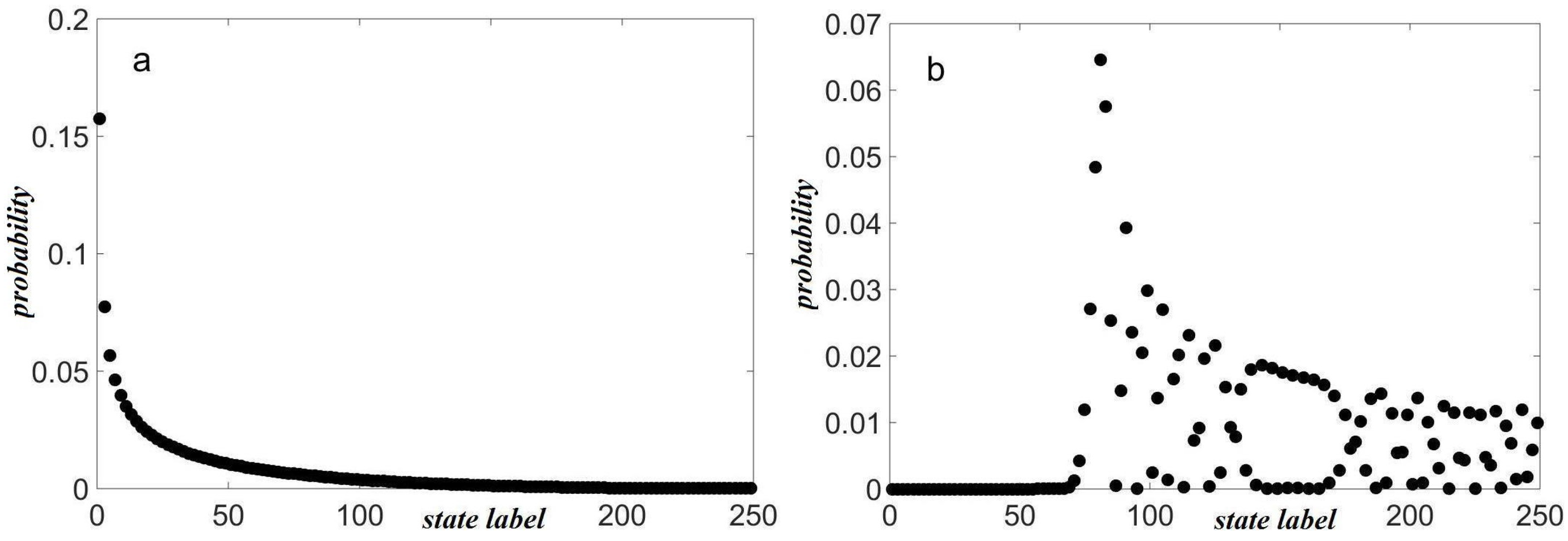
Figure 2.
(a) 500 points are started in the square and , but are otherwise randomly selected. After one time step under the cat map, Equation (3), they have become the parallelogram in (b). They have stretched in the direction of the eigenvector with larger eigenvalue of M (Equation (3)) and shrunk by the inverse of the stretching factor along the other eigenvector. (The product of the eigenvalues is 1 because . The dynamics therefore mimic Hamiltonian dynamics in that it satisfies Liouville’s theorem.) (c) By time 3, the mod 1 action coupled with the stretching has begun to pull the points apart and; (d) by time 7, nothing is recognizable.
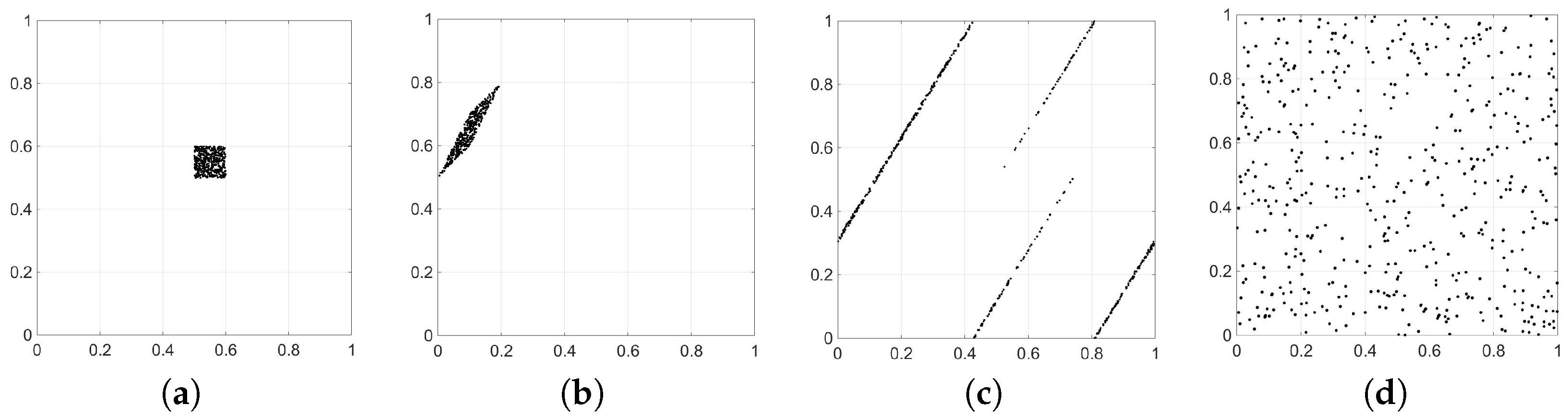
Figure 3.
Entropy, as defined in Equation (4), as a function of time for the simulation of Figure 2. For this grain size, equilibration sets in at about time-5. The dashed figure is the maximum entropy for this coarse graining, namely . It is not attained because the number of points is finite.

Figure 4.
The times are as follows: (a–d) [0, 1, 2, 4]; (e–h) [6, 7, 8, 9]; (i–l) [10, 11, 12, 14]; (m–p) [15, 16, 17, 18]. These points all evolve under the cat map and satisfy boundary conditions at times 0, 9 and 18. The size of the position marker (a point) varies with the image for better visibility.
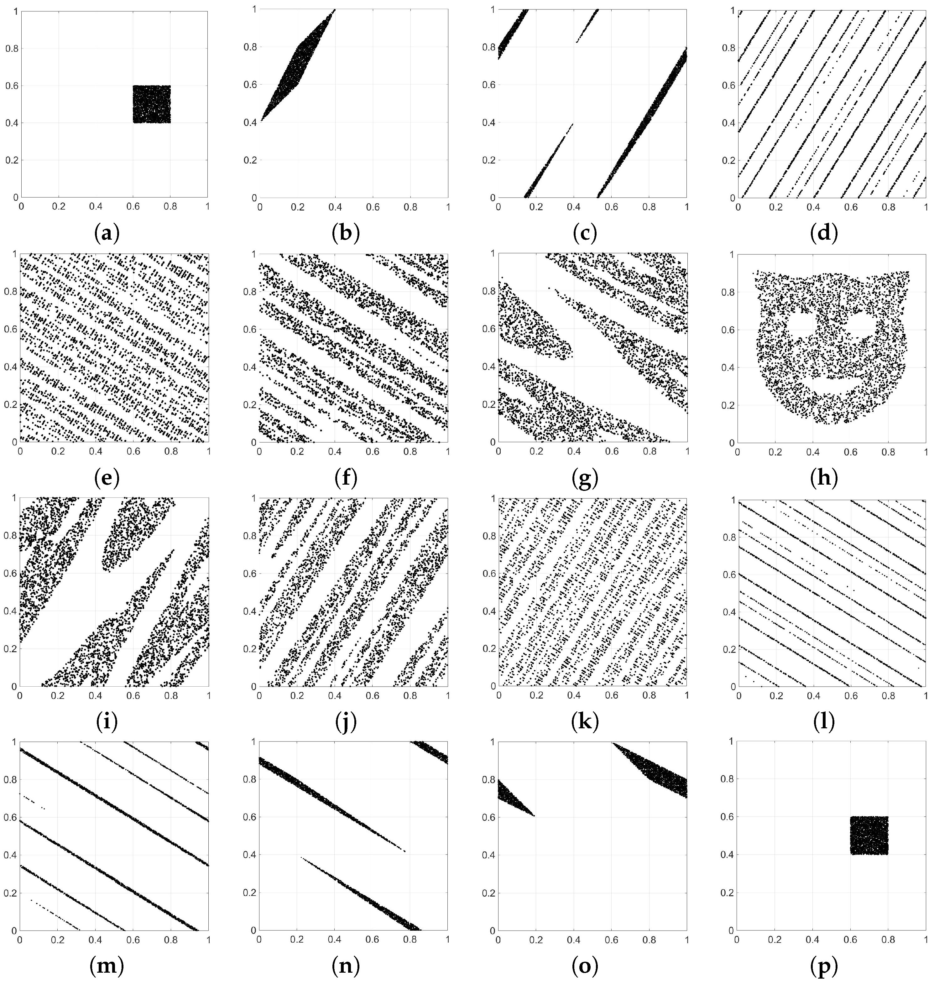
Figure 5.
The circles and solid line represent the entropy as a function of time for the simulation shown in Figure 4. Note that it drops a bit at time-9 and then at time-18 goes to 0, since all points are again in a single grain. The other curve, marked by stars, is the entropy as a function of time for 4000 points having the same initial grain, but with no other constraints.
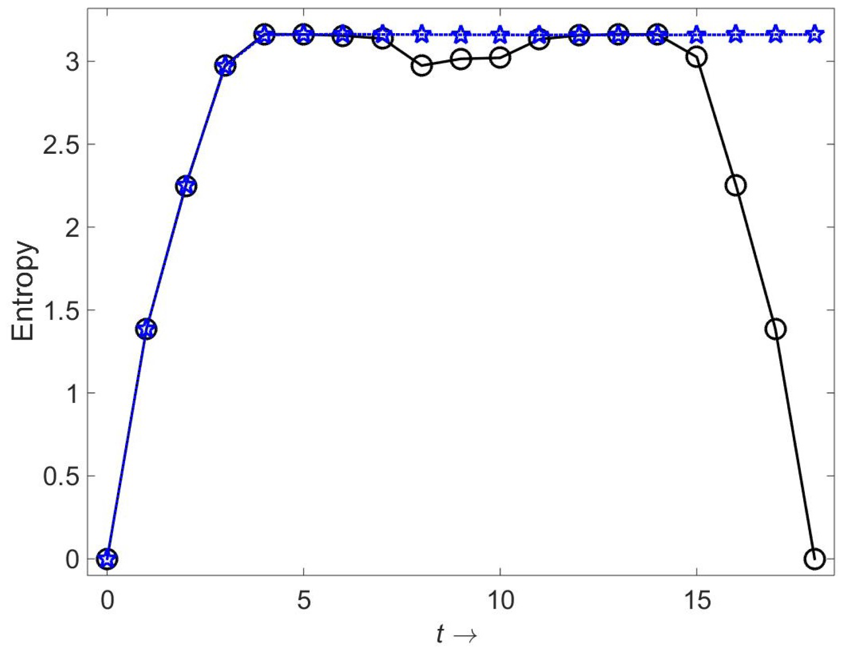
Figure 6.
Cat map entropy as a function of time for several final time constraints. In each case, points are started in a single box and required to end in another such box. As is evident, the relaxation time is about 5 time units and if the boundary conditions are separated by twice that time, no anomaly is observed. However, when the boundary value constraint is for shorter times, the entropy never reaches its maximum and anomalies are noted.

© 2017 by the author. Licensee MDPI, Basel, Switzerland. This article is an open access article distributed under the terms and conditions of the Creative Commons Attribution (CC BY) license (http://creativecommons.org/licenses/by/4.0/).
Share and Cite
MDPI and ACS Style
Schulman, L.S. Program for the Special State Theory of Quantum Measurement. Entropy 2017, 19, 343. https://doi.org/10.3390/e19070343
AMA Style
Schulman LS. Program for the Special State Theory of Quantum Measurement. Entropy. 2017; 19(7):343. https://doi.org/10.3390/e19070343
Chicago/Turabian StyleSchulman, Lawrence S. 2017. "Program for the Special State Theory of Quantum Measurement" Entropy 19, no. 7: 343. https://doi.org/10.3390/e19070343
Note that from the first issue of 2016, this journal uses article numbers instead of page numbers. See further details here.