Iterant Algebra


Department of Mathematics, Statistics and Computer Science, University of Illinois at Chicago, 851 South Morgan Street, Chicago, IL 60607-7045, USA
Entropy 2017, 19(7), 347; https://doi.org/10.3390/e19070347
Submission received: 29 May 2017
/
Revised: 26 June 2017
/
Accepted: 5 July 2017
/
Published: 11 July 2017
(This article belongs to the Special Issue Quantum Information and Foundations)
Abstract
:We give an exposition of iterant algebra, a generalization of matrix algebra that is motivated by the structure of measurement for discrete processes. We show how Clifford algebras and matrix algebras arise naturally from iterants, and we then use this point of view to discuss the Schrödinger and Dirac equations, Majorana Fermions, representations of the braid group and the framed braids in relation to the structure of the Standard Model for physics.
1. Introduction
This is a paper about an approach to algebra that we call iterants. The idea behind the definition of iterant (see Section 2) is that one is studying a periodic discrete process with an associated action of a group of permutations on the sequences of the process. The simplest such discrete system is an alternation between and We will show that this system gives rise in a natural way to the square root of minus one. This way thinking about the square root of minus one as an iterant is explained below. More generally, by starting with a discrete time series of positions, one has a non-commutativity of observations due to time-delays (the clock must tick to measure a velocity) and this non-commutativity can be encapsulated in a generalized iterant algebra as defined in Section 3 of the present paper. Iterant algebra generalizes matrix algebra and we shall see how it can be used to formulate the algebra of the framed Artin Braid Group, the Lie algebra for the Standard Model for particle physics, the framed braid representations for Fermions of Sundance Bilson-Thompson, the Clifford algebra for Majorana Fermions and the structure of the Schrödinger and Dirac equations. This paper is a sequel to [1] and it uses material from that paper and extends it into the more general context of the present paper. See also [1,2,3,4] for previous work by the author about iterants. This paper also incorporates results of the author that appear in the joint paper of the author and Rukhsan Ul-Haq [5]. Our intent is to give a picture of the range of application of the basic mathematical idea of iterants and to include a description of the basic results that make them work.
This paper is organized as follows. Section 2, Section 3 and Section 4 are devoted to the mathematics of iterants. Each remaining section of the paper applies the iterant structure to a topic in mathematical physics that is of interest to the author. We hope that the reader finds the first few sections to be a readable introduction to iterants. An interested reader can then turn to the remaining sections to see how iterants can be used in specific cases. The reader should note that since applying iterants often means reformulating a topic usually written in matrix algebra in terms of iterant algebra, and the specific interest in such a formulation may be, at this time, of a formal nature. Nevertheless, the reformulation often raises many interesting questions, and these will be the subject of subsequent work.
Section 2 and Section 3 are an introduction to the process algebra of iterants and how the square root of minus one arises from an alternating process. Section 4 shows how iterants give an alternative way to do matrix algebra. The section ends with the construction of the split quaternions. Section 4 considers iterants of arbitrary period (not just two) and shows, with the example of the cyclic group, how the ring of all matrices can be seen as a faithful representation of an iterant algebra based on the cyclic group of order We then generalize this construction (Theorem 1) to arbitrary non-commutative finite groups Such a group has a multiplication table ( where n is the order of the group G). We show that, by rearranging the multiplication table so that the identity elements appear on the diagonal, we get a set of permutation matrices that represent the group faithfully as matrices. This gives a faithful representation of the iterant algebra associated with the group G onto the ring of matrices. As a result, we see that iterant algebra is fundamental to matrix algebra. Section 4 ends with a number of classical examples including iterant representations for quaternion algebra.
Section 5 is a discussion of the Schrödinger equation. We formulate a discrete model related to the diffusion equation by following a heuristic that would identify the square root of minus one as a controlled oscillation between plus one and minus one. The resulting discrete model has the equation (compare with [1])
and satisfies a discrete version of the diffusion equation with an extra coefficient of , where denotes the number of time steps needed to reach time By dividing this discrete system into its even and odd parts (the parity of ), we retrieve the Schrödinger equation, and the formalism of the complex numbers handles the parity. In the discrete model, the iterant structure appears directly.
Section 6 discusses the iterant structure of the framed Artin braid group via framed braids and discusses the basics of the Sundance Bilson-Thompson model for elementary particles. In Section 7, we apply this to a formulation of the particle model of Sundance Bilson-Thompson [6], using framed braids.
In Section 7, we give an iterant interpretation of the Lie algebra for the Standard Model using [7]. The resulting formulation of the Lie algebra is particularly elegant from our point of view, and we expect it to give further insight into the standard model. This iterant formulation of the Lie Algebra is so concise that we show it here in the Introduction. We use the specific iterant formulas
We have the permutation relations and so that This reduces the basic Lie algebra to a very elementary patterning of order three cyclic operations. The details of this formulation are given in Section 7.
In Section 8, we apply this point of view on the Standard Model to obtain an embedding of the framed braid algebra for the Sundance Bilson-Thompson model into the iterant version of These three sections are an account of research of the author and Rukhsan Ul-Haq in [5].
Section 9 discusses how Clifford algebras are related to the structure of Fermions. We show how the algebra of the split quaternions, the very first iterant algebra that appears in relation to the square root of minus one, is behind the structure of the operator algebra of the electron. The Clifford structure on two generators describes a pair of Majorana Fermion operators. Majorana Fermions are particles that are their own antiparticles. These Majorana Fermion operators correspond to Clifford algebra generators a and b such that and Using our iterant formulation, we can take a as the iterant corresponding to a period two oscillation, and b as the time shifting operator. The product is a square root of minus one in the non-commutative context of this Clifford algebra. The annihilation operator for an electron can be symbolized by and the creation operator for an electron by These form the operator algebra for an electron. Note that
and therefore
The electron is seen in terms of its underlying Clifford structure in the form of a pair of Majorana Fermions. Section 9 shows how braiding is related to the Majorana Femions.
Section 10 discusses the structure of the Dirac equation and how the nilpotent and the Majorana operators arise naturally in this context. This section provides a link between our work and the work on nilpotent structures and the Dirac equation of Peter Rowlands [8]. We end this section with an expression in split quaternions for the the Majorana–Dirac equation in spacetime. The Majorana–Dirac equation can be written as follows:
where and are the generators of our simplest iterant algebra with and The elements form a commuting copy of this algebra. This use of a combination of the simplest Clifford algebra with itself is the underlying structure of the Majorana–Dirac equation.
We give a specific real solution to the Majorana–Dirac equation in our iterant/Clifford algebra formalism. Here, , where is a constant vector momentum, and x denotes the vector The solution to the Majorana–Dirac equation is as shown below:
This solution is real in the sense that its coordinates are all real valued functions once the iterant or matrix forms for the operators are made explicit. The combination of iterant and Clifford algebra language that we develop here makes the analysis of certain aspects of the Dirac equation and the Majorana–Dirac equation very clear. More work needs to be done in all these fronts.
This paper is a snapshot of a larger story. Iterant algebra is a basically simple reformulation of aspects of patterned algebra that can often illuminate correspondingly elementary topics in mathematics and physics. The present work is a beginning in the larger enterprise of understanding relationships in discrete physics and relationships between algbra and physics.
2. Iterants
An iterant is a sum of elements of the form
where is a vector of elements that are scalars (usually real or complex numbers) and is a permutation on n letters. Vectors are added and multiplied coordinatewise (see below), and we take the following rule for multiplication of vector/permutation combinations:
where denotes the vector b with its elements permuted by the action of
If a and b are vectors, then denotes the vector, where and denotes the vector where Then,
for a scalar k, and
where vectors are multiplied as above and we take the usual product of the permutations. All of matrix algebra is naturally represented in the iterant framework, as we shall see in the next sections.
For example, if is the order two permutation of two elements, then Thus,
We define
and then
In this way, the complex numbers arise naturally from iterants. One can interpret as an oscillation between and and as a temporal shift operator. Then, is a time sensitive element and its self-interaction has square minus one. In this way, iterants can be interpreted as a formalization of elementary discrete processes.
Note that if we let then and Thus, e and generate a small Clifford algebra.
3. Iterants and Discrete Processes
The primitive idea behind an iterant is a periodic time series or “waveform”
We illustrate with period two. The elements of the waveform can be any mathematically or empirically well-defined objects. We can regard the ordered pairs and as abbreviations for the waveform or as two points of view about the waveform (a first or b first). We have called an iterant. Thinking of an iterant as a discrete process, we define a time shift operator such that and
Discrete Calculus and the Temporal Shift Operator. If we have a discrete time series then it is convenient to define an operator J so that , and it is this temporal shift operator that can be used to correlate discrete calculus for the time-series. For example, we can define a discrete derivative D by the equation
(with time increment equal to ). Note then that the derivative is expressed as a commutator:
where here is the commutator. This means that this discrete derivative satisfies the Leibniz rule for products, and it can be used for formulations of discrete physics. This use of the temporal shift operator dovetails with its use for keeping track of observation in a discrete model, where successive observations require temporal shifts. In particular, let and denote momentum and position, respectively (m is mass and commutes with as does ). Then, and do not commute and the temporal shift operator J keeps track of the fact that measuring momentum requires a tick of the clock. We can interpret as first measuring Q and then measuring P, while represents first measuring P and then measuring
Thus,
In this form of discrete physics, the commutator equation
where k is a constant, is satisfied by a Brownian walk with diffusion constant In this way, our interpretation of the square root of negative one in terms of the temporal shift operator fits into a larger context of the physics of discrete observations. In this paper, we work with periodic series and use cyclic operators such as to keep track of the periodicity. For related discussion, see [2,3,5,9,10,11,12,13,14,15,16]. See also [17] for other uses of iterants in the context of Clifford algebras. For papers of the author about discrete physics and quantum computing see [18,19,20,21,22,23,24,25,26,27,28].
We have defined products and sums of iterants as follows
and
The operation of juxtapostion of waveforms is multiplication while + denotes ordinary addition of ordered pairs. These operations are natural with respect to the structural juxtaposition of iterants:
Structures combine at the points where they correspond. Waveforms combine at the times where they correspond. Iterants combine in juxtaposition. This theme of including the result of time in observations of a discrete system occurs at the foundation of our construction.
In the next section, we show how all matrix algebra can be formulated in terms of iterants.
4. Matrix Algebra via Iterants
Here is a direct translation of period-two iterants into matrices. Let
where
and
The reader will have no difficulty verifying that the usual definition of matrix multiplicaiton corresponds exactly to the iterant multiplication that we have already described. In particular,
and
are rules of matrix multiplication and addition, as are
Thus, matrix multiplication and addition is identical with iterant multiplication. There are many ways to motivate the rules for matrix algebra. Iterants are a natural entry into matrix structure.
The fact that the iterant expression captures the whole of matrix algebra corresponds to the fact that a two by two matrix is combinatorially the union of the identity pattern (the diagonal) and the interchange pattern (the antidiagonal) that correspond to the operators 1 and
In the formal diagram for a matrix shown above, we indicate the diagonal by ∗ and the anti-diagonal by
In the case of complex numbers, we represent
In this way, we see that matrix algebra can be seen as a hypercomplex number system based on the symmetric group In the next section, we generalize this point of view to arbitrary finite groups by generalizing Cayley’s Theorem that shows that every finite group has a faithful representation as a permutation group.
The factorization of i into a product of non-commuting iterant operators shows, in the iterant viewpoint, the temporal nature of i and its algebraic roots.
Note that the quaternions arise from the split quaternions: The split quaternions are the system
Here, while so that . The quaternions come about once we construct an extra square root of minus one that commutes with them. Call this extra root of minus one . Then, the quaternions are generated by
with
Remark 1.
The rest of this section is an exposition of the higher period iterants and the general Theorem 1 about finite groups and iterant matrix representations. The exposition follows the corresponding exposition in our paper [1].
4.1. Iterants of Arbirtarily High Period and General Matrix Algebras
Consider a waveform of period three.
Here, we see three natural iterant views (depending upon whether one starts at a, b or c).
The appropriate shift operator is given by the cyclic permutation S:
With we have
and We obtain a closed algebra of iterants whose general element is of the form
where are real or complex numbers. Call this algebra when the scalars are in a commutative ring with unit Let denote the matrix algebra over We have the:
Lemma 1.
The iterant algebra is isomorphic to the full matrix algebra
Proof.
maps to the matrix
preserving the algebra structure. Since any matrix can be written uniquely in this form, it follows that is isomorphic to the full matrix algebra ☐
We can summarize the pattern behind this expression of matrices by the following symbolic matrix:
Here, the letter T occupies the positions in the matrix that correspond to the permutation matrix that represents it, and the letter occupies the positions corresponding to its permutation matrix. The 1s occupy the diagonal for the corresponding identity matrix. The iterant representation corresponds to writing the matrix as a disjoint sum of these permutation matrices such that the matrices themselves are closed under multiplication. In this case, the matrices form a permutation representation of the cyclic group of order 3,
Remark 2.
Note that a permutation matrix is a matrix of zeroes and ones such that some permutation of the rows of the matrix transforms it to the identity matrix. Given an permutation matrix we associate to it a permuation
via the following formula
where j denotes the column in P where the i-th row has a 1. Note that an element of the domain of a permutation is indicated to the left of the symbol for the permutation. It is then easy to check that for permutation matrices P and Q,
given that we compose the permutations from left to right according to this convention.
This construction generalizes directly for iterants of any period and hence for a set of operators forming a cyclic group of any order. We shall generalize further to any finite group We now define for any finite group
Definition 1.
Let G be a finite group, written multiplicatively. Let denote a given commutative ring with unit. Assume that G acts as a group of permutations on the set so that given an element we have (by abuse of notation)
We shall write
for the image of under the permutation represented by The notation denotes functionality from the left. We have for all elements and for all i, in order to have a representation of G as permutations. We shall call an n-tuple of elements of a vector and denote it by We then define an action of G on vectors over by the formula
and note that for all Define an algebra , the iterant algebra for G, to be the set of finite sums of formal products of vectors and group elements in the form with multiplication rule
and the understanding that and for all vectors and group elements It is understood that vectors are added coordinatewise and multiplied coordinatewise. Thus, and
Theorem 1.
Let G be a finite group of order n [1]. Let denote the right regular representation of G as permutations of n objects. List the elements of G as and let G act on its own underlying set via the definition Here, we describe acting on the set of elements of We also regard as a mapping of the set , replacing by k and where
Then, is isomorphic to the matrix algebra In particular, is isomorphic with the matrices of size ,
Proof.
Take the multiplication table for G to be the matrix with columns and rows listed in the order Permute the rows of this matrix so that the diagonal consists in all 1 s. Let the resulting matrix be called the G-Table. The G-Table is labeled by elements of the group. For any vector let denote the diagonal matrix whose entries in order down the diagonal are the entries of a in the order specified by For each group element g, let denote the permutation matrix with 1 in every spot on the G-Table that is labeled by g and 0 in all other spots. It is now a direct verification that the mapping
defines an isomorphism from to the matrix algebra The main point to check is that We now prove this fact.
In the G-Table, the rows correspond to and the columns correspond to so that the i-i entry of the table is With this, we have that, in the table, a group element g occurs in the i-th row at column j where This is equivalent to the equation which, in turn, is equivalent to the statement This is exactly our functional interpretation of the action of the permutation corresponding to the matrix Thus, The rest of the proof is straightforward and left to the reader. ☐
Example 1.
- 1.
- Consider the cyclic group of order three.with The multiplication table isInterchanging the second and third rows, we obtainand this is the G-Table that we used for prior to proving the Main Theorem. The same pattern works for abitrary cyclic groups.
- 2.
- Consider the symmetric group on six letters,where Then, the multiplication table isThe corresponnding G-Table isThis G-Table encodes the isomorphism of with the full algebra of six by six matrices. Similarly, is isomorphic with the full algebra of matrices. The permutation matrices are obtained from the G-Table by choosing a given group element and then replacing it by 1 for each appearance in the table, and replacing the other elements of the table by For example, we have the permutation matrix for R given by the formula below:
- 3.
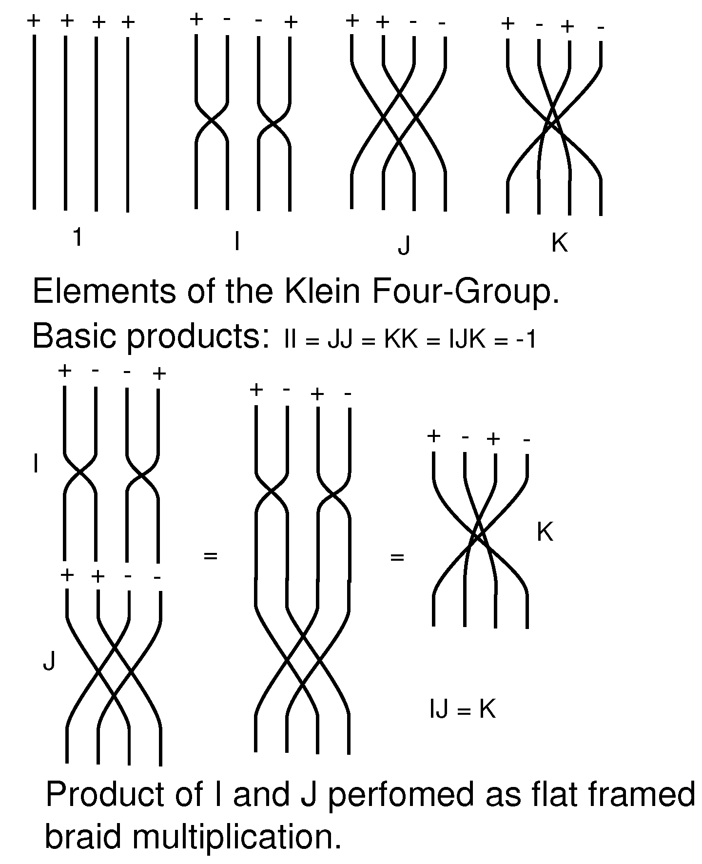
- Consider the group the “Klein 4-Group”. Take where , G has the multiplication table, which is also its G-Table forThus, we have the corresponding permutation matrices that I shall call The reader can verify that LetIn addition, letThen, it is easy to check thatThus, we have constructed the quaternions as iterants in relation to the Klein 4-Group. In Figure 1, we illustrate these quaternion generators with string diagrams for the permutations. The reader can check that the permuations correspond to the permutation matrices constructed for the Klein 4-Group.
- 4.
- Since complex numbers commute with one another, we could consider iterants whose values are in the complex numbers. This is just like considering matrices whose entries are complex numbers. Thus, we shall allow a version of i that commutes with the iterant shift operator Let this commuting i be denoted by Then, we are assuming thatWe then consider iterants of the form and In particular, we have and is quite distinct from Note, as before, that and that Now, letWe find the quaternions once more:Thus,This construction shows how the structure of the quaternions comes directly from the non-commutative structure of period two iterants. The group of unitary matrices of determinant one is isomorphic to the quaternions of length one.
- 5.
- Similarly,represents a Hermitian matrix and hence an observable for quantum processes mediated by Hermitian matrices have real eigenvalues.If in the above Hermitian matrix form, we take then we obtain an iterant and/or matrix representation for a point in Minkowski spacetime:Note that we have the formulaIt is not hard to see that the eigenvalues of H are Thus, viewed as an observable, H can observe the time and the invariant spatial distance from the origin of the event At least at this very elementary juncture, quantum mechanics and special relativity are reconciled.
- 6.
- Hamilton’s Quaternions are generated by iterants, as discussed above, and we can express them purely algebraicially by writing the corresponding permutations as shown below:whereHere, we represent the permutations as products of transpositions The transposition interchanges i and leaving all other elements of fixed.One can verify thatNote that making an iterant interpretation of an entity like is a conceptual departure from our original period two iterant (or cyclic period n) notion. Now, we consider iterants such as where the permutation group acts to produce other orderings of a given sequence. The iterant itself can represent a form that can be seen in any of its possible orders. These orders are subject to permutations that produce the possible views of the iterant. Algebraic structures such as the quaternions appear in the explication of such forms.
- 7.
- In all these examples, we can interpret the iterants as short hand for matrix algebra based on permutation matrices, or as indicators of discrete processes. The discrete processes become more complex in proportion to the complexity of the groups used in the construction. We began with processes of order two, then considered cyclic groups of arbitrary order, then the symmetric group in relation to matrices, and the Klein 4-Group in relation to the quaternions. In the case of the quaternions, we know that this structure is intimately related to rotations of three- and four-dimensional space and many other geometric themes.
5. Schrödinger’s Equation
In this section, we go more deeply into a treatment of Schrödinger’s equation that was begun in the introduction to [1]. In that paper, we used this example for Schrödinger’s equation to motivate the introduction of iterants. Here, we already have iterants, but we find that a discrete model for Schrödinger’s equation instantiates an alternating pattern that is essentially of the form and the problem of taking the continuum limit of this discrete model leads to the complex numbers by a parity consideration. The parity consideration corresponds to our iterant construction of the square root of minus one, and so we see in this model how the iterant square root of minus one can correspond to an alternation in a discrete process while the usual square root of minus one describes the behaviour of the limit of the process.
5.1. Brownian Walks and the Diffusion Equation
Recall how the diffusion equation arises in discussing Brownian motion. We are given a Brownian process where
so that the time step is and the space step is of absolute value We regard the probability of left or right steps as equal, so that if denotes the probability that the Brownian particle is at point x at time t, then
From this equation for the probability, we can write a difference equation for the partial derivative of the probability with respect to time:
The expression in brackets on the right-hand side is a discrete approximation to the second partial of with respect to Thus, if the ratio remains constant as the space and time intervals approach zero, then this equation goes in the limit to the diffusion equation
C is called the diffusion constant for the Brownian process.
5.2. An Iterant Intepretation of Schrödinger’s Equation
Recall that Schrödinger’s equation can be regarded as the diffusion equation with an imaginary diffusion constant. Recall how this works. The Schrödinger equation is
where the Hamiltonian H is given by the equation , where is the potential energy and is the momentum operator. With this, we have Thus, with , the equation becomes , which simplifies to
Thus, we have arrived at the form of the diffusion equation with an imaginary constant, and it is possible to make the identification with the diffusion equation by setting
where denotes a space interval, and denotes a time interval as explained in the last section about the Brownian walk. With this, we can ask what space interval and time interval will satisfy this relationship? One answer is that this equation is satisfied when m is the Planck mass, is the Planck length and is the Planck time. Note that Here, ℏ is Planck’s constant divided by c is the speed of light. G is Newton’s gravitational constant.
What does all this say about the nature of the Schrödinger equation itself? Consider a discrete function defined (recursively) by the following equation:
In other words, we are thinking here of a random “quantum walk” where the amplitude for stepping right or stepping left is proportional to i while the amplitude for not moving at all is proportional to It is then easy to see that is a discretization of
Just note that satisfies the difference equation
This gives a direct interpretation of the solution to the Schrödinger equation as a limit of a sum over generalized Brownian paths with complex amplitudes.
Replacing i by An Iterant. Now, however, suppose that we replace i by at time step where is a non-negative integer. Instead of writing
we will write
Then, we will find that
so that the diffusion equation seems to have been replaced with an equation of the form
We wish to consider the continuum limit. However, there is no meaning to
in the realm of continuous time. In the discrete world, the wave function divides into and where the (discrete) time, is either even or odd. We write
and take the continuum limit of and separately.
In fact, we can interpret the as the complex number We write
so that
Thus,
This the Schrödinger equation. Instead of the simple diffusion equation, we have a mutual dependency where the temporal variation of is mediated by the spatial variation of and vice-versa:
Note that in terms of the iterant interpretation, the pair is an abbreviation of the temporal series that represents the discrete process Here, the process itself is not periodic, but the underlying alternation of the parity of gives the iterant stucture that allows the use of i as a combination of shift and permutation.
Remark 3.
The discrete recursion at the beginning of this section can be implemented to approximate solutions to the Schrödinger equation. This will be the subject of another paper. The main point of this section is that a discrete version of the Schrödinger equation actually uses the temporal iterant interpretation of the square root of minus one, so that one can think of this oscillation as part of a discrete process in back of the Schrödinger evolution. This reformulation of basic quantum mechanics deserves further study.
6. The Framed Braid Group and the Sundance Bilson-Thompson Model for Elementary Particles
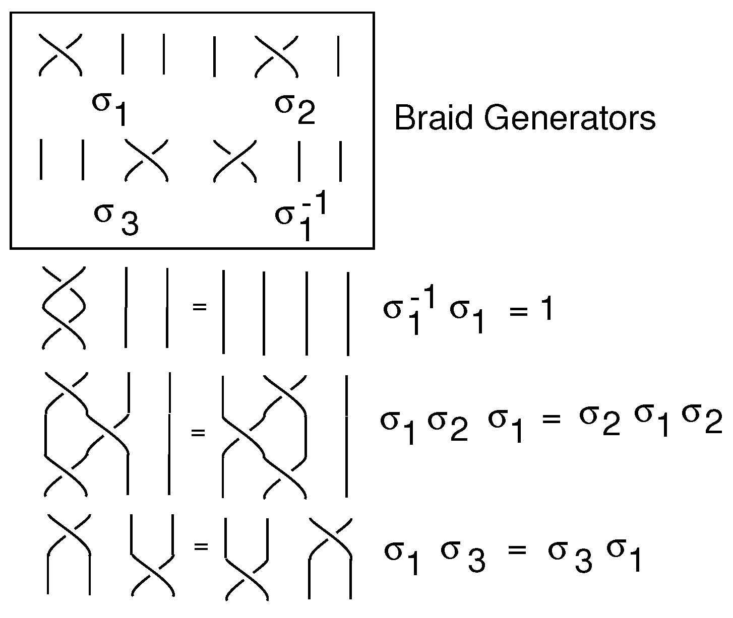
The reader should recall that the symmetric group has presentation
The Artin Braid Group is a relative of the symmetric group that is obtained by removing the condition that each generator has a square equal to the identity:
In Figure 2, we illustrate the the generators of the 4-strand braid group and we show the topological nature of the relation and the commuting relation Topological braids are represented as collections of always descending strings, starting from a row of points and ending at another row of points. The strings are embedded in three-dimensional space and can wind around one another. The elementary braid generators correspond to the i-th strand interchanging with the ()-th strand. Two braids are multiplied by attaching the bottom endpoiints of one braid to the top endpoints of the other braid to form a new braid.
There is a fundamental homomorphism
defined on generators by
in the language of the presentations above. In terms of the diagrams in Figure 2, a braid diagram is a permutation diagram if one forgets about its weaving structure of over and under strands at a crossing.
We now turn to a generalization of the braid group, the framed braid group. In this generalization, we associate elements of the form to the top of each braid strand. For these purposes, it is useful to take t as an algebraic variable and a as an integer. To interpret this framing, geometrically replace each braid strand by a ribbon and interpret as a twist in the ribbon. In Figure 3, we illustrate how to multiply two framed braids. In our formalism, the braids A and B in this figure are given by the formulas
in the framed braid group on three strands, denoted As the Figure 3 illustrates, we have the basic formula
where v is a vector of the form (for ) and denotes the action of the permutation associated with the braid on the vector In the figure, the permutation is accomplished by sliding the algebra along the strings of the braid.
We can form an algebra by taking formal sums of framed braids of the form where is a scalar, is a framing vector and is an element of the Artin Braid group Since braids act on framing vectors by permutations, this algebra is a generalization of the iterant algebras we have defined so far. The algebra of framed braids uses an action of the braid group based on its representation to the symmetric group. Furthemore, the representation induces a map of algebras
where we recognize as exactly an iterant algebra based in
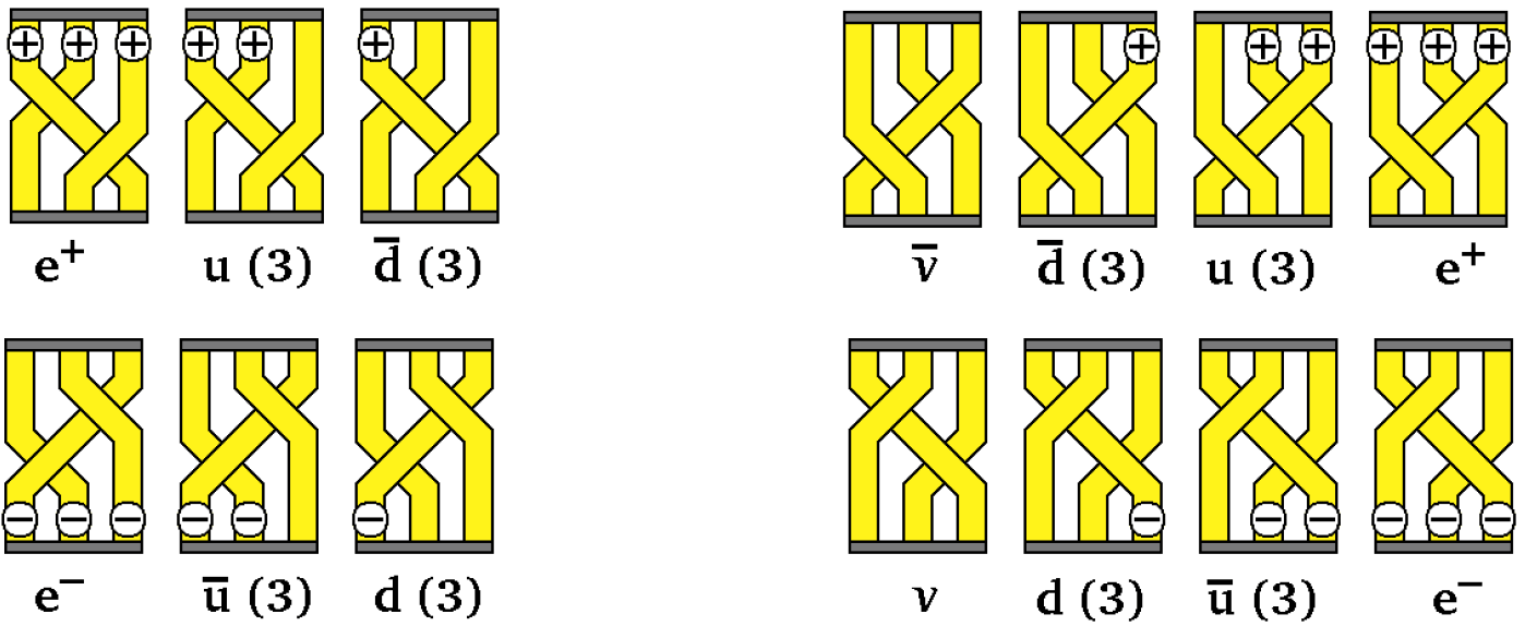
In [6], Sundance Bilson-Thompson represents Fermions as framed braids. See Figure 4 for his diagrammatic representations. In this theory, each Fermion is associated with a framed braid. Thus, from the figure, we see that the positron and the electron are given by the framed braids
and
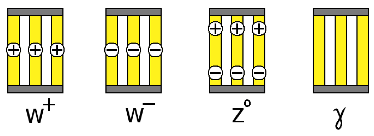
Here, we use for the framing numbers Products of framed braids correspond to particle interactions. Note that so that the electron and the positron are inverses in this algebra. In Figure 5 are illustrated the representations of bosons, including , a photon and the identity element in this algebra. Other relations in the algebra correspond to particle interactions. For example, in Figure 6 the muon decay is illustrated:
The reader can see the definitions of the different parts of this decay sequence from the three figures we have just mentioned. Note that strictly speaking the muon decay is a multiplicative identity in the braid algebra:
Particle interactions in this model are mediated by factorizations in the non-commutative algebra of the framed braids.
By using the representation we can image the structure of Bilson-Thompson’s framed braids in the the iterant algebra corresponding to the symmetric group. However, we propose to change this map so that we have a non-trivial representation of the Artin braid group. This can be accomplished by defining
where
and
for The reader will find that we have now represented the braid group in the iterant algebra and extended the representation to the framed braid group algebra. Thus, the Sundance Bilson-Thompson representation of elementary particles as framed braids is represented inside the iterant algebra for the symmetric group on three letters. In Section 10, we carry this further and place the representation inside the Lie Algebra
7. Iterants and the Standard Model
In this section, we shall give an iterant interpretation for the Lie algebra of the special unitary group The Lie algebra in question is denoted as and is often described by a matrix basis. The Lie algebra is generated by the following eight Gell Man Matrices [29]:
The group consists of the matrices where are real numbers and a ranges from 1 to The Gell Man matrices satisfy the following relations:
Here, we use the summation convention summing over repeated indices, and denotes standard matrix trace, is the matrix commutator and is the Kronecker delta, equal to 1 when , and equal to 0, otherwise. The structure coefficients take the following non-zero values:
We now give an iterant representation for these matrices that is based on the pattern
as described in the previous section. That is, we use the cyclic group of order three to represent all matrices at iterants based on the permutation matrices
Recalling that as an iterant, denotes a diagonal matrix
the reader will have no difficulty verifying the following formulas for the Gell Mann Matrices in the iterant format:
Letting we can now rewrite the Lie algebra into simple iterants of the form where G is a cyclic group element. Compare with [7]. Let
Iterant Formulation of the Lie Algebra. We now have the specific iterant formulas
We have that and so that We have reduced the basic Lie algebra to a very elementary patterning of order three cyclic operations. In a subsequent paper, we will use this point to view to examine the irreducible representations of this algebra and to illuminate the Standard Model’s Eightfold Way.
8. Iterants, Braiding and the Sundance Bilson-Thompson Model for Fermions
In the last section, we based our iterant representations on the following patterns and matrices. The pattern,
uses the cyclic group of order three to represent all matrices at iterants based on the permutation matrices
Recalling that as an iterant denotes a diagonal matrix
In fact, there are six permuation matrices: where
We then have The two transpositions P and Q generate the entire group of permuatations It is usual to think of the order-three transformations A and B as expressed in terms of these transpositons, but we can also use the iterant structure of the matrices to express Q and R in terms of A and The result is as follows:
Recall from the previous section that we have the iterant generators for the Lie algebra:
Thus, we can express these transpositions P and Q in the iterant form of the Lie algebra as
The basic permutations receive elegant expressions in the iterant Lie algebra.
Now that we have basic permutations in the Lie algebra, we can take the map from Section 7
with
and
for and send to P and to Q. Then, we have
and
and
and
By choosing on the unit circle in the complex plane, we obtain representations of the Sundance Bilson-Thompson constructions of Fermions via framed braids inside the Lie algebra. This brings the Bilson-Thompson formalism in direct contact with the Standard Model via our iterant representations. We shall return to these relationships in a sequel to the present paper.
9. Clifford Algebra, Majorana Fermions and Braiding
This section is based on our paper [1]. We show how the very simple Clifford algebra(s) that come from iterants figure in studying Fermions and Majorana Fermions. This section also provides the background for the next section on the Dirac equation. The original paper by Ettore Majorana [30] led to the notion of Clifford algebraic Majorana operators that we discuss in this section. In the next section on the Dirac equation, we show how this Clifford algebra is related to Majorana’s original equation. A key relationship between the physics of the Quantum Hall effect and the kind of braiding representations considered here originates with the paper of Moore and Read [31]. See also [28] where we look at the combinatorial topology behind the braid group representations of Moore and Read.
Recall Fermion algebra. One has Fermion annihiliation operators and their conjugate creation operators One has There is a fundamental commutation relation
If you have more than one of them, say and , then they anti-commute:
Majorana Fermion operators c satisfy so that the corresponding particles are their own anti-particles. A group of researchers [32] claims, at this writing, to have found Majorana Fermions in edge effects in nano-wires.
Majorana operators are related to standard Fermions as follows: the algebra for Majoranas is and if c and are distinct Majorana Fermions with and One can make a standard Fermion operator from two Majorana operators via
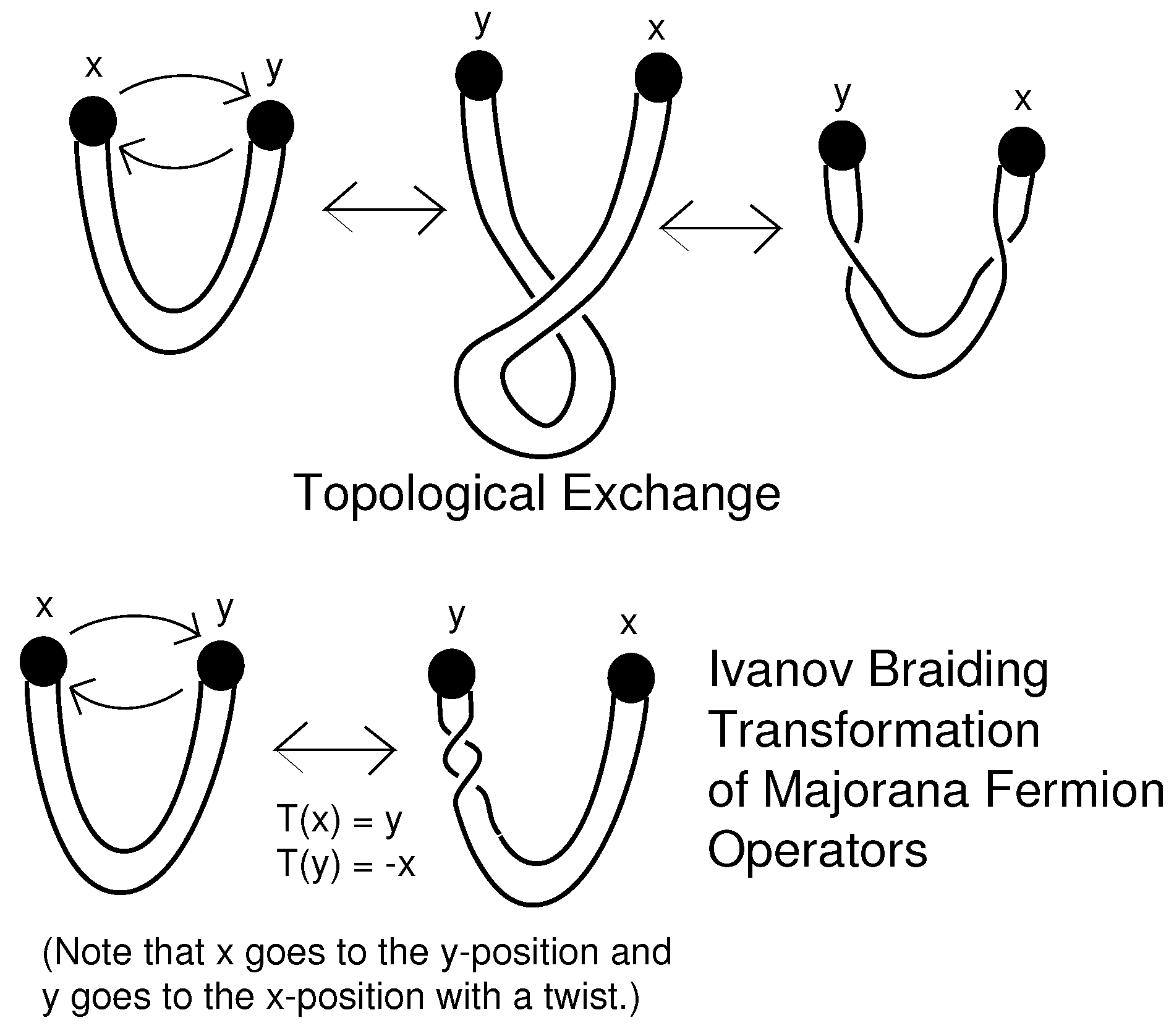
Similarly, one can mathematically make two Majoranas from any single Fermion. If one takes a set of Majoranas
then there are natural braiding operators that act on the vector space with these as the basis. The operators are mediated by algebra elements that themselves satisfy braiding relations
The Ivanov [33] braiding operators are
via
The braiding is simply:
and is the identity otherwise. We have then a unitary representaton of the Artin braid group. See Figure 7 for a depiction of the braiding of Majorana Fermions in relation to the topology of a belt that connects them. In quantum mechanics, we must represent rotations of three-dimensional space as unitary transformations. This relationship between rotations and unitary transformations is encoded in the topology of the belt. See [34] for more about this topological view of the physics of Fermions. In the figure, we see that the strictly topological belt does not know which of the two Fermions will individually acquire a phase change, but the Ivanov algebra above makes this decision. More understanding is needed in this area of subtle topological structure of Fermions.
Recall that, in discussing the inception of iterants, we introduce a temporal shift operator such that
and
for any iterant In this way, we have a Clifford algebra generated by and We can take e and as Majorana Fermion operators and construct Fermion operators
Here, i is an extra square root of minus one that commutes with the operators e and We arrive at fermions in a few short steps from the origin of the iterants. Algebraically, we have controlled the period two oscillation e so that it satisfies the fermion algebra. From the point of view taken in this paper, it is worth examining if this discrete process view of fermion algebra and Majorana operator algebra can shed light on the many properties in this domain. In particular, I would like to see if there is insight into the braiding of Majorana Fermion operators to be gained from the iterant viewpoint.
10. The Dirac Equation and Majorana Fermions
This section goes beyond our paper [1]. We expand on the relationship of a nilpotent formulation of the Dirac equation and an iterant formulation. We first construct the Dirac equation. The algebra underlying this equation has the same properties as the creation and annihilation algebra for Majorana Fermion operators, so it is by way of this algebra that we will come to the Dirac equation.
If the speed of light is equal to 1 (by convention), then energy E, momentum p and mass m are related by the (Einstein) equation
Dirac constructed his equation by finding an algebraic square root of A corresponding linear operator for E can then take the role of the Hamiltonian in the Schrödinger equation. We first assume that p is a scalar (using one dimension of space and one dimension of time). Let where and are elements of a non-commutative, associative algebra. Then,
Hence, if and We can use the iterant algebra generated by e and with and Recall that the quantum operator for momentum is and the operator for energy is The Dirac equation is
This becomes the explicit equation:
Let
so that the Dirac equation takes the form
A Plane Wave Solution to the Dirac Equation. Note that
and note also that
Thus, it follows that
is a solution of the Dirac equation.
Now let and let
Then,
The nilpotent element U leads to the same plane wave solution to the Dirac equation as follows. We have shown that
for It then follows that
from which it follows that
is a plane wave solution to the Dirac equation.
We can multiply the operator by on the right, obtaining the operator
and the equivalent Dirac equation
For above, we have This beautiful observation that the Dirac operator can be modified so that one can directly construct nilpotent solutions to the Dirac equation was first made by Peter Rowlands [8] in the context of doubled quaternion algebra. Here we have shown how Rowland’s work fits into the Clifford algebra and iterant approach to the Dirac equation. Such solutions can be articulated into specific vector solutions by using either an iterant or matrix representation of the algebra.
10.1. U and as Creation and Annihilation Operators
The Clifford algebra element U can be regarded (in the context of this rewrite of the Dirac equation) as a creation operator for a Fermion.
If, reversing time, we let
then
giving a definition of for the anti-particle for
and
Note that here we have
and
and
The Fermion operator algebra emerges from these plane wave solutions to the Dirac equation. The decomposition of U and into the corresponding Majorana Fermion operators corresponds to the decomposition of the energy into momentum and mass: Normalizing by dividing by , we have
and
so that
and
Then,
and
showing how the Fermion operators are expressed in terms of the simpler Clifford algebra of Majorana operators (split quaternions once again). We can take and and regard these Fermion annihilation and creation operators in the simplest iterant framework.
10.2. Iterant Formulation of the Dirac Equation
Note that the solutions to the Dirac equation that we have written are expressed using abstract algebra. To write explicit solutions using this algebraic approach, we can write
where is the energy operator and is the momentum operator. Then, a solution
of the Dirac equation consists in a quadruple of complex functions of such that
We can regard as an iterant that is acted upon by and . We see that (by multiplying on the left)
and
Thus, the structure corresponds to the action of the split quaternions as a signed Klein 4-group. The equation becomes four operator equations involving these signed permutations:
Thus, is equivalent to the set of equations
This, in turn, can be written in iterant form as
The plane wave solution k corresponds, in this iterant formalism, to
In this way, we can think of a solution to the Dirac equation as an iterant composed of four complex valued functions taken in order with the given action of the split quaternions as described above. This can then be reformulated as single recursive system, as we did for the Schrödinger equation in the introduction. The analogs for the way the recursion acts on the time steps of the recursion are given by the action of the split quaternions rather than the action of the complex numbers (). The idea remains the same, and the matrix representations for the Dirac algebra arise naturally from the algebra itself.
10.3. Writing in the Full Dirac Algebra
This section closely follows our paper [1] and is expanded for the discussion at the end. The aim is to write the Dirac equation for three dimensions of space and one dimension of time, and then to write a version of the Majorana–Dirac Equation (that can have real solutions) in terms of a doubled split quaternion algebra, expressed in iterant language. This provides an alternative to working with modifications of the Dirac matrices. We formulate it to illustrate again the iterant concept and to raise the question of finding other matrix representations for equations of Majorana type.
We have written the Dirac equation so far in one dimension of space and one dimension of time. In order to write in three spatial dimensions, we take an independent Clifford algebra generated by with for and for Assume that and generate an independent Clifford algebra that commutes with the algebra of the Replace the scalar momentum p by a 3-vector momentum and let = Replace with and with
The Dirac equation is then written
The Dirac operator is
Using the Dirac operator, the Dirac equation is is
Let
and construct solutions by first applying the Dirac operator to this The modified Dirac operator is
We have that
where Here, and is a solution to the modified Dirac Equation. We can use the Fermion operators as creation and annihilation operators, and locate the corresponding Majorana Fermion operators. We leave these details to the reader.
10.4. Majorana Fermions in the Sense of Majorana
We end with a brief discussion making Dirac algebra distinct from the one generated by to obtain an equation that can have real solutions. This was the strategy that Majorana [30] followed to construct his Majorana Fermions. A real equation can have solutions that are invariant under complex conjugation and so can correspond to particles that are their own anti-particles. We will describe this Majorana algebra in terms of the split quaternions and For convenience, we use the matrix representation given below. The reader of this paper can substitute the corresponding iterants:
Let and generate another, independent algebra of split quaternions, commuting with the first algebra generated by and Then, a totally real Majorana Dirac equation can be written as follows:
To see that this is a correct Dirac equation, note that
(Here, the “hats” denote the quantum differential operators corresponding to the energy and momentum.) will satisfy
if the algebra generated by has each generator of square one and each distinct pair of generators anti-commuting. From there, we obtain the general Dirac equation by replacing by , and with (and same for ):
This is equivalent to
Thus, here we take
and observe that these elements satisfy the requirements for the Dirac algebra. Since the algebra appearing in the Majorana–Dirac operator is constructed entirely from two commuting copies of the split quaternions, there is no appearance of the complex numbers, and when written out in matrices, we obtain coupled real differential equations to be solved.
A solution to the Majorana–Dirac Equation. Let Note that is a a real-valued function. Let
This is the Majorana–Dirac operator, as we have explained above. Then, we have the equation
Let
and
Then, we have
since all algebraic coefficients square to minus one, and anti-commute. Therefore,
Thus,
is a solution to the Majorana–Dirac equation. When this solution is written out into its components, it is an entirely real valued solution since the components of the matrices representing the algebra are all real numbers. Recall from the earlier part of this section that we were able to reformulate solutions of this kind for the usual Dirac equation in terms of the nilpotent formalism with the algebraic element U with Here, we can produce real solutions to the Majorana–Dirac equation, but it does not seem possible to put them in the nilpotent formalism. This is surely a reflection of the fact that these solutions are not Fermions in the usual sense. On the other hand, one can regard the solution in relation to the algebra element and this algebra element is a combination of Majorana Fermion operators in the sense of Clifford algebra or iterant operators that we have used earlier in this paper. Thus, we see that there is at least the beginning of a relationship between the modern use of the Majorana Fermion operators and the original intents of Ettore Majorana to find real solutions to the Dirac equation.
We would like to know if there are other ways to produce such real Dirac equations, and particularly if there are ways to accomplish this aim that do not algebraically entangle the two copies of the split quaternions as our construction (and Majorana’s original construction) seems to require.
Acknowledgments
It gives the author great pleasure to thank G. Spencer-Brown, James Flagg, Alex Comfort, David Finkelstein, Pierre Noyes, Peter Rowlands, Sam Lomonaco, Bernd Schmeikal and Rukhsan Ul-Haq for conversations related to the considerations in this paper.
Conflicts of Interest
The author declares no conflict of interest.
References
- Kauffman, L.H. Iterants, Fermions and Majorana Operators. In Unified Field Mechanics—Natural Science Beyond the Veil of Spacetime; Amoroso, R., Kauffman, L.H., Rowlands, P., Eds.; World Scientific Pub. Co.: Singapore, 2015; pp. 1–32. [Google Scholar]
- Kauffman, L.H. Knot Logic. In Knots and Applications; Kauffman, L., Ed.; World Scientific Pub. Co.: Singapore, 1994; pp. 1–110. [Google Scholar]
- Kauffman, L.H. Knot logic and topological quantum computing with Majorana fermions. In Logic and Algebraic Structures in Quantum Computing and Information; Lecture Notes in Logic; Chubb, J., Eskandarian, A., Harizanov, V., Eds.; Cambridge University Press: Cambridge, UK, 2016; 124p. [Google Scholar]
- Kauffman, L.H.; Lomonaco, S.J. Braiding, Majorana Fermions and Topological Quantum Computing, (to appear in Special Issue of QIP on Topological Quantum Computing). In Proceedings of the 2nd International Conference and Exhibition on Mesoscopic and Condensed Matter Physics, Chicago, IL, USA, 26–28 October 2016. [Google Scholar]
- Ul Haq, R.; Kauffman, L.H. Iterants, Idempotents and Clifford algebra in Quantum Theory. arXiv, 2017; arXiv:1705.06600. [Google Scholar]
- Bilson-Thompson, S.O. A topological model of composite fermions. arXiv, 2006; arXiv:hep-ph/0503213. [Google Scholar]
- Gasiorowicz, S. Elementary Particle Physics; Wiley: New York, NY, USA, 1966. [Google Scholar]
- Rowlands, P. Zero to Infinity: The Foundations of Physics; Series on Knots and Everything, Volume 41; World Scientific Publishing Co.: Singapore, 2007. [Google Scholar]
- Spencer-Brown, G. Laws of Form; George Allen and Unwin Ltd.: London, UK, 1969. [Google Scholar]
- Kauffman, L. Sign and Space. In Religious Experience and Scientific Paradigms, Proceedings of the 1982 IASWR Conference; Institute of Advanced Study of World Religions: Stony Brook, NY, USA, 1985; pp. 118–164. [Google Scholar]
- Kauffman, L. Self-reference and recursive forms. J. Soc. Biol. Struct. 1987, 10, 53–72. [Google Scholar] [CrossRef]
- Kauffman, L. Special relativity and a calculus of distinctions. In Proceedings of the 9th Annual International Meeting of ANPA, Cambridge, UK, 23–28 September 1987; pp. 290–311. [Google Scholar]
- Kauffman, L. Imaginary values in mathematical logic. In Proceedings of the Seventeenth International Conference on Multiple Valued Logic, Boston, MA, USA, 26–28 May 1987; pp. 282–289. [Google Scholar]
- Kauffman, L.H. Biologic. AMS Contemp. Math. Ser. 2002, 304, 313–340. [Google Scholar]
- Kauffman, L.H. Temperley-Lieb Recoupling Theory and Invariants of Three-Manifolds (Annals Studies-114); Princeton University Press: Princeton, NJ, USA, 1994. [Google Scholar]
- Kauffman, L.H. Time imaginary value, paradox sign and space. In Computing Anticipatory Systems, Proceedings of the AIP Conference CASYS—Fifth International Conference, Liege, Belgium, 13–18 August 2001; Dubois, D., Ed.; AIP Conference Publishing: Melville, NY, USA, 2002; Volume 627. [Google Scholar]
- Schmiekal, B. Decay of Motion: The Anti-Physics of SpaceTime; Nova Publishers, Inc.: Hauppauge, NY, USA, 2014. [Google Scholar]
- Kauffman, L.H.; Noyes, H.P. Discrete Physics and the Derivation of Electromagnetism from the formalism of Quantum Mechanics. Proc. R. Soc. Lond. A 1996, 452, 81–95. [Google Scholar] [CrossRef]
- Kauffman, L.H.; Noyes, H.P. Discrete Physics and the Dirac Equation. Phys. Lett. A 1996, 218, 139–146. [Google Scholar] [CrossRef]
- Kauffman, L.H. Noncommutativity and discrete physics. Phys. D Nonlinear Phenom. 1998, 120, 125–138. [Google Scholar] [CrossRef]
- Kauffman, L.H. Space and time in discrete physics. Int. J. Gen. Syst. 1998, 27, 241–273. [Google Scholar] [CrossRef]
- Kauffman, L.H. A non-commutative approach to discrete physics. In Aspects II: Proceedings of ANPA 20; ANPA: Stanford, CA, USA, 1999; pp. 215–238. [Google Scholar]
- Kauffman, L.H. Non-commutative calculus and discrete physics. In Boundaries: Scientific Aspects of ANPA 24; ANPA: Stanford, CA, USA, 2003; pp. 73–128. [Google Scholar]
- Kauffman, L.H. Non-commutative worlds. New J. Phys. 2004, 6, 73. [Google Scholar] [CrossRef]
- Kauffman, L.H. Non-commutative worlds and classical constraints. In Scientific Essays in Honor of Pierre Noyes on the Occasion of His 90-th Birthday; Amson, J., Kaufman, L.H., Eds.; World Scientific Pub. Co.: Singapore, 2013; pp. 169–210. [Google Scholar]
- Kauffman, L.H. Differential geometry in non-commutative worlds. In Quantum Gravity: Mathematical Models and Experimental Bounds; Fauser, B., Tolksdorf, J., Zeidler, E., Eds.; Birkhauser: Basel, Switzerland, 2007; pp. 61–75. [Google Scholar]
- Kauffman, L.H. Knot Logic and Topological Quantum Computing with Majorana Fermions. arXiv, 2013; arXiv:1301.6214. [Google Scholar]
- Kauffman, L.H.; Lomonaco, S.J., Jr. q-deformed spin networks, knot polynomials and anyonic topological quantum computation. J. Knot Theory Ramif. 2007, 16, 267–332. [Google Scholar] [CrossRef]
- Cheng, T.P.; Lee, L.F. Gauge Theory of Elementary Particles; Clarendon Press: Oxford, UK, 1988. [Google Scholar]
- Majorana, E. A symmetric theory of electrons and positrons. I Nuovo Cimento 1937, 14, 171–184. [Google Scholar] [CrossRef]
- Moore, G.; Read, N. Noabelions in the fractional quantum Hall effect. Nucl. Phys. B 1991, 360, 362–396. [Google Scholar] [CrossRef]
- Mourik, V.; Zuo, K.; Frolov, S.M.; Plissard, S.R.; Bakkers, E.P.A.M.; Kouwenhuven, L.P. Signatures of Majorana fermions in hybred superconductor-semiconductor devices. Science 2012, 336, 1003–1007. [Google Scholar] [CrossRef] [PubMed]
- Ivanov, D.A. Non-abelian statistics of half-quantum vortices in p-wave superconductors. Phys. Rev. Lett. 2001, 86, 268. [Google Scholar] [CrossRef] [PubMed]
- Kauffman, L.H. Knots and Physics; World Scientific Pub., Co.: Singapore, 2012. [Google Scholar]
Figure 1.
Quaternions from the Klein 4-Group.

Figure 2.
Braid generators.

Figure 3.
Framed braids.
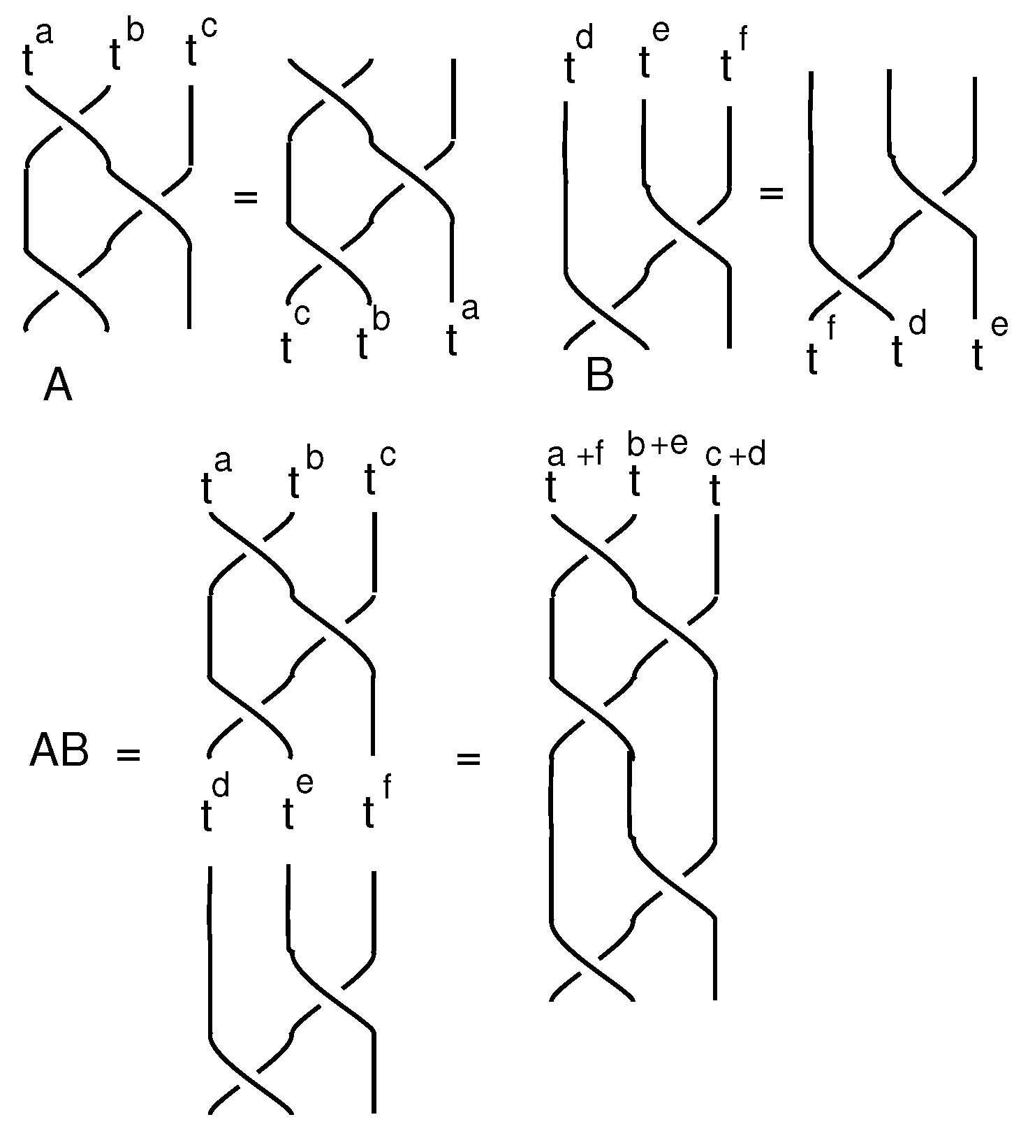
Figure 4.
Sundance Bilson-Thompson Framed Braid Fermions (“(3)” under the labels for the up and down quarks and antiquarks represent the fact that there are three permutations of charge placement giving the three colours).
Figure 4.
Sundance Bilson-Thompson Framed Braid Fermions (“(3)” under the labels for the up and down quarks and antiquarks represent the fact that there are three permutations of charge placement giving the three colours).

Figure 5.
Bosons.

Figure 6.
Representation of
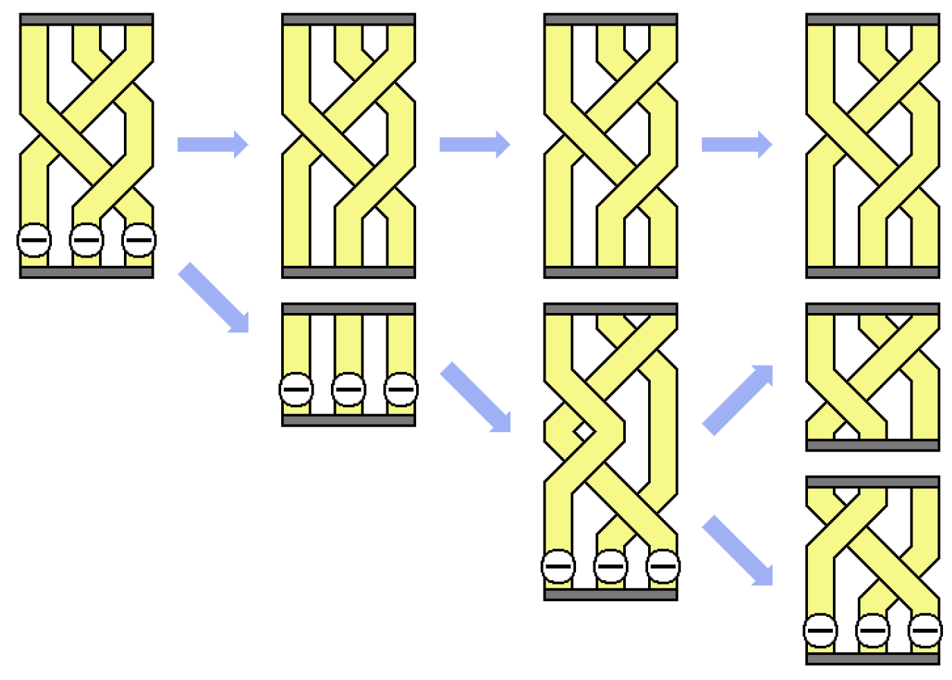
Figure 7.
Braiding action on a pair of fermions.
© 2017 by the author. Licensee MDPI, Basel, Switzerland. This article is an open access article distributed under the terms and conditions of the Creative Commons Attribution (CC BY) license (http://creativecommons.org/licenses/by/4.0/).
Share and Cite
MDPI and ACS Style
Kauffman, L.H. Iterant Algebra. Entropy 2017, 19, 347. https://doi.org/10.3390/e19070347
AMA Style
Kauffman LH. Iterant Algebra. Entropy. 2017; 19(7):347. https://doi.org/10.3390/e19070347
Chicago/Turabian StyleKauffman, Louis H. 2017. "Iterant Algebra" Entropy 19, no. 7: 347. https://doi.org/10.3390/e19070347
Note that from the first issue of 2016, this journal uses article numbers instead of page numbers. See further details here.