Discrete Wigner Function Derivation of the Aaronson–Gottesman Tableau Algorithm

Department of Physics, Tufts University, Medford, MA 02155, USA
*
Author to whom correspondence should be addressed.
Entropy 2017, 19(7), 353; https://doi.org/10.3390/e19070353
Submission received: 3 May 2017
/
Revised: 28 June 2017
/
Accepted: 4 July 2017
/
Published: 11 July 2017
(This article belongs to the Special Issue Quantum Information and Foundations)
Abstract
:The Gottesman–Knill theorem established that stabilizer states and Clifford operations can be efficiently simulated classically. For qudits with odd dimension three and greater, stabilizer states and Clifford operations have been found to correspond to positive discrete Wigner functions and dynamics. We present a discrete Wigner function-based simulation algorithm for odd-d qudits that has the same time and space complexity as the Aaronson–Gottesman algorithm for qubits. We show that the efficiency of both algorithms is due to harmonic evolution in the symplectic structure of discrete phase space. The differences between the Wigner function algorithm for odd-d and the Aaronson–Gottesman algorithm for qubits are likely due only to the fact that the Weyl–Heisenberg group is not in for and that qubits exhibit state-independent contextuality. This may provide a guide for extending the discrete Wigner function approach to qubits.
1. Introduction
The cost of brute-force classical simulation of the time evolution of n-qubit states grows exponentially with n. An important exception to this involves the set of Clifford operators acting on stabilizer states. This set of states plays an important role in quantum error correction [1] and is closed under action by Clifford gates. Efficient simulation of such systems was demonstrated with the tableau algorithm of Aaronson and Gottesman [1,2] for qubits (). Finding the underlying reason for why such an efficient algorithm is possible for Clifford circuit simulation has since been the subject of much study [3,4,5].
Recent progress has been the result of work by Wootters [6], Gross [7], Veitch et al. [8,9], Mari et al. [4], and Howard et al. [5], who have formulated a new perspective based on the discrete phase spaces of states and operators in finite Hilbert spaces using discrete Wigner functions. In odd-dimensional systems, they have shown that stabilizer states have positive-definite discrete Wigner functions and that Clifford operators are positive-definite maps. This implies that Clifford circuits are non-contextual and are efficiently simulatable on classical computers. In odd-dimensional systems, stabilizer states have been shown to be the discrete analogue to Gaussian states in continuous systems [7] and Clifford group gates have been shown to have underlying harmonic Hamiltonians that preserve the discrete Weyl phase space points [10]. This means Clifford circuits are expressible by path integrals truncated at order and are thus manifestly classical [10,11].
This poses the question: what is the relationship between past efficient algorithms for Clifford circuits and the propagation of discrete Wigner functions of stabilizer states under Clifford operators? In the present paper, we show that the original Aaronson–Gottesman tableau algorithm for qubit stabilizer states is actually equivalent to such a discrete Wigner function propagation and that the tableau matrix coincides with the discrete Wigner function of a stabilizer state. We accomplish this by first developing a Wigner function-based algorithm that classically simulates stabilizer state evolution under Clifford gates and measurements in the Pauli basis for odd d. We then show its equivalence to the well-known Aaronson–Gottesman tableau algorithm [2] for qubits (). Both algorithms require dits to represent n stabilizer states, operations per Clifford operator, and both deterministic and random measurements require operations.
The Aaronson–Gottesman tableau algorithm makes use of the Heisenberg representation. This means that time evolution is accomplished by updating an associated tableau or matrix representation of the Clifford operators instead of the stabilizer states themselves. The algorithm we present is framed in the Schrödinger picture and involves evolving the Wigner function of stabilizer states. By demonstrating that the two algorithms are equivalent, we show that the formulation of Clifford simulation in the Heisenberg picture is a choice and not a necessity for its efficient simulation. Furthermore, by instead working in the Schrödinger picture we are able to more easily reveal the purely classical basis of both algorithms and the physically intuitive phase space structures and symplectic properties on which they rely.
2. Discrete Wigner Function for Odd d Qudits
Before we discuss the discrete Wigner function, we introduce a basic framework that defines how a phase space behaves for odd d-dimensional Hilbert spaces. To begin, we associate the computational basis with the position basis, such that the Pauli operator on the jth qudit for n qudits acts as a “boost” operator:
where for .
The discrete Fourier transform operator is defined by:
This is the d-dimensional equivalent of the Hadamard gate and allows us to define the Pauli operator as follows:
While is a boost, is a shift operator because
where ⊕ denotes integer addition mod d.
We can reexpress the boost and shift operators in terms of their generators, which are the conjugate and operators, respectively:
and
Thus, we can refer to the basis as the momentum () basis, which is equivalent to the Fourier transform of the basis:
These bases form the discrete Weyl phase space .
The Wigner function of a pure state is defined on this discrete Weyl phase space:
This is equivalent to the discrete Wigner function introduced by Gross [7]. We will shortly be interested in the discrete Wigner function of stabilizer states. However, first, we introduce the effect that the Clifford gates have in this discrete Weyl phase space.
2.1. Clifford Gates
A Clifford group gate is related to a symplectic transformation on the discrete Weyl phase space, governed by a symplectic matrix and vector [7]:
Wigner functions of states evolve under Clifford operators by
where . When considering Clifford gate propagation, we can restrict to a set of gates which are generators of the Clifford group. One such set of generators is made up of the phase-shift gate , the Hadamard gate , and the controlled-not (CNOT) (which act on the ith and jth qudits).
The phase shift is a one-qudit gate with the underlying Hamiltonian [10]. Without loss of generality, we will instead consider
which we will refer to as the phase-shift gate in this paper. We note that the usual phase-shift can be obtained from the new one within the Clifford group:
where . Hence, is an adequate replacement generator for , and we will use it instead of from now on. Since its Hamiltonian has no linear term (), this leads to an easier presentation ahead since . The corresponding equations of motion for are and . Hence, for ,
The Hadamard gate is a one-qudit gate and has the underlying Hamiltonian [10]. The corresponding equations of motion are and . Hence, for ,
and .
Finally, the two-qudit CNOT on control qudit i and second qudit j has the corresponding Hamiltonian [10]. The corresponding equations of motion are and . Hence, for ,
and .
2.2. Wigner Functions of Stabilizer States
A discrete Wigner function for stabilizer states associated with the boost and shift operators defined in Equations (4) and (5) is given by the following theorem [10]:
Theorem 1.
The discrete Wigner function of a stabilizer state Ψ for any odd d and n qudits is for matrix Φ and vector with entries in .
An equivalent form was proven by Gross [7] who also showed that these discrete Wigner functions of stabilizer states are non-negative. In particular, if we begin with a stabilizer state defined as , then , where for the identity matrix, and .
3. Wigner Stabilizer Algorithm for Odd d Qudits
With the discrete Wigner function of a stabilizer state defined in Theorem 1 and the effect of the Clifford group generators on discrete Wigner functions defined in Equation (9), we can now examine the effect Clifford operators have on stabilizer states. We note that since the discrete Wigner functions of stabilizer states are non-negative and Clifford operations take stabilizer states to stabilizer states, it follows that Clifford operations (if associated positive-operator valued measures (POVMs) also have non-negative Wigner functions) can always be efficiently classically simulated by sampling from these Wigner functions as probability distributions [4]. However, here we pursue a description that is not dependent on classical sampling.
3.1. Stabilizer Representation
From Theorem 1, propagation of the stabilizer state can be represented by considering the state’s Wigner function: . In this way, and specify a linear system of equations in terms of and . The first n rows of are the coefficients of in and the last n rows of are the coefficients of in :
The Kronecker delta function sets this linear system of equations equal to . In this way, an affine map—a linear transformation displaced from the origin by —is defined. This system of equations must be updated after every unitary propagation and measurement.
Since the Wigner functions of stabilizer states propagate under as , it follows that
(The importance of vector and when it must be updated will become evident when we consider random measurements.) Hence, after n operations , , …, ,
The matrices are ordered chronologically left-to-right instead of right-to-left.
Since is symplectic, where
Thus, the the stability matrices for , and given in Equations (12)–(14) differ from their inverses only by sign changes in their off-diagonal elements:
and
We assume the quantum state is initialized in the computational basis state and so initially we should set and . The initial stabilizer state is . However, it will become clear when we discuss measurements that it is practically useful to instead set
thereby setting —not a true Wigner function. This new matrix is equivalent to the last matrix if the first n rows in and are ignored—the same as ignoring . In fact, we have two Wigner functions here: one defined by the first n rows and another by the last n rows. We proceed in this manner, ignoring the first n rows, until their usefulness becomes apparent to us.
For n qudits unitary propagation requires dits of storage to track and . More precisely, since is a matrix and is an -vector, dits of storage are necessary.
3.2. Unitary Propagation
contains the coefficients of the linear equations relating to . Each row is one equation relating or to . When manipulating rows of we shall refer to the linear equations that these rows define.
Examining Equations (19)–(21), we see that the inverse stability matrices of the generator gates , and are the sum of an identity matrix and a matrix with a finite number of non-zero off-diagonal elements. The number of these off-diagonal elements is independent of the number of qudits, n. Hence, multiplying with a new stability matrix in Equation (16) and evaluating the matrix multiplication is equivalent to performing a finite number of n-vector dot products and so requires operations. Therefore, keeping track of propagation of stabilizer states by Clifford gates can be simulated with operations.
Let us examine these unitary operations more closely. Defining ⊕ and ⊖ to be mod d addition and subtraction respectively, we find:
Phase gate on qudit i (). For all , set .
Hadamard gate on qudit i (). For all , negate mod d, and then swap and .
CNOT from control i to target j (). For all , set and .
This confirms that unitary propagation in this scheme requires operations.
3.3. Measurement
The outcome of a measurement on a stabilizer state can be either random or deterministic. As described above, the bottom half of defines for , each of which is a linear combination of and . The entries in the th row of give the coefficient of and in for . If the coefficient of in any is non-zero then the measurement will be random. If all coefficients of are zero for , then the measurement of will be deterministic. This can be seen from the fact that if our stabilizer state is an eigenstate of , then for some and (discrete) Wigner functions do not change under a global phase. Thus, measuring leaves the Wigner function of invariant if the measurement is deterministic. Since is a boost operator that increments the momentum of a state by one, its effect on the linear system of equations specified by the Wigner function is:
Thus, if the lower half of the ith column of is zero, then leaves the Wigner function invariant (and so the measurement is deterministic). Verifying that these coefficients are all zero takes operations for each .
In other words, to see if a given measurement of is random or deterministic, a search must be performed for non-zero elements. If such a non-zero element exists, then the measurement is random since it means that the final momentum of qudit i affects the state of the stabilizer and so its position must be undetermined (by Heisenberg’s uncertainty principle). If no such finite element exists, then the measurement is deterministic. We now describe the algorithm in detail for these two cases:
Case 1: Random Measurement
Let the th row in the bottom half of have a non-zero entry in the ith column, . Since the random measurement will project qudit i onto a position state, we will replace the th row with (the uniformly random outcome of this measurement). After this projection onto a position state, none of the other qudits’ positions should depend on qudit i’s momentum, . To accomplish this, before we replace row , we solve its equation for and substitute every instance of in the linear system of equations with this solution. As a result, every equation will no longer depend on and we can go ahead and replace the th row with .
There is one more thing to do, which will be important for deterministic measurements: replace the jth row with the old th row. This sets , which becomes the only remaining equation explicitly dependent on . In other words, , similar to the beginning when we set by setting . However, now we also preserve any dependence has on the other qudits incurred during unitary propagation. In other words, we preserve ’s dependence upon the other qudits, but only in the Wigner function specified by the top n rows, which we ignore otherwise.
After replacing the equation specified by row of and with a randomly chosen measurement outcome (i.e., ), the identification of rows and are exchanged, so that the former now specifies while the latter specifies . has also been updated by replacing the jth row in the first half of , with the th row we just changed. Again, this row now describes while the ith row now specifies . Overall, this takes operations since we are replacing rows with entries.
Case 2: Deterministic Measurement
Since the measurement is deterministic, and do not change. The n equations specified by the bottom half of can be used to solve for —the deterministic measurement outcome. In general, this can also be done by inverting and evaluating for . Aaronson and Gottesman themselves noted that such a matrix inversion is possible, but practically takes operations. (However, we are not certain if Aaronson and Gottesman were referring to the matrix corresponding to the part of their tableau when they discuss matrix inversion in [2].)
Fortunately, there is another method that scales as and requires use of the n equations represented by the top n rows of , which were included in our description by setting . The linear system of n equations represented by can be written as
where we are interested in linear combinations of the bottom half, , to solve for the measurement outcome :
where .
Lemma 1.
The coefficient in front of in the row of that specifies , , is equal to the coefficient in front of that makes up in Equation (26). Equivalently,
Proof.
Under evolution under the Clifford group operators,
since is symplectic. This means that we can express the matrix inversion as follows:
Therefore, , and so
This property can also be seen in the drawing of phase space shown in Figure 1. There, initial perpendicular and manifolds are drawn along with harmonically evolved and manifolds, which remain perpendicular to each other and make an angle to the first and manifolds, respectively. The projection of onto can be represented as the length b of a right triangle’s adjacent side to the angle , with an opposite side set to some length a. The projection of onto is similarly represented by the length of a right triangle’s adjacent side to the angle , with an opposite side also set to length a. It follows that the third angle in both triangles must be the same, and so by the law of sines
Therefore, and so these two projections are equal to one another. In the discrete Weyl phase space such manifolds must lie along grid phase points and obey the periodicity in and , but the premise is the same. ☐
Overall, the procedure outlined in Lemma 1 for deterministic measurements takes operations since Equation (27) is a sum of vectors made up of components. Therefore, the overall measurement protocol takes operations. Note that this formulation of the algorithm shows that it is the symplectic structure on phase space and the linear transformation under harmonic evolution that allows the inversion (Equation (32)) to be performed efficiently.
4. Aaronson–Gottesman Tableau Algorithm for Qubits ()
The Aaronson–Gottesman tableau algorithm was originally defined for qubits () [2]. Like the algorithm we presented in the previous section, it only requires overall operations for propagation and measurement for n qubits. The algorithm has been proven to be extendable to [12] and similar algorithms have been formulated in [13]. Alternatives have also been developed to the tableau formalism, though they prove to be equally efficient in worst-case scenarios [14]. However, we are not aware of any direct extension of the Aaronson–Gottesman tableau algorithm to dimensions greater than two. In this and the next section, we will show that the Wigner algorithm presented in Section 3 is equivalent to the Aaronson–Gottesman tableau algorithm extended to odd d.
4.1. Stabilizer Representation
The Aaronson–Gottesman algorithm is defined in the stabilizer formalism. It keeps track of the evolution of a stabilizer state by updating the generators of the stabilizer group, elements of which are defined as follows:
Definition 1.
A set of operators that satisfies such that are called the stabilizers of state , where is the set of Pauli operators, each of which has the form where for n qubits with .
For the sake of completeness, we present here a summary of the qubit Aaronson–Gottesman algorithm, in order to compare it to our odd d qudit algorithm. For more details, see [1,2].
Each n-qubit stabilizer state is uniquely determined by Pauli operators. There are only n generators of this Abelian group of operators. Therefore, an n-qubit stabilizer state is defined by the n generators of its stabilizer state. Every element in this set of generators, , is in the Pauli group, and each generator has the form:
Any unitary propagation by Clifford operators or measurement of the stabilizer state changes at least some of the elements of the n generators of the state’s stabilizer. This includes the phase in Equation (35), which must also be kept track of in Aaronson–Gottesman’s algorithm.
4.2. Unitary Propagation
For each Clifford operation, Aaronson and Gottesman showed that only operations are necessary to update all generators [2]. Specifically, according to the update rules in Table 1, each generator can be updated with a constant number of operators for every single Clifford gate, therefore in total. However, it is a little more complicated to update the generators after each measurement. To do this efficiently, Aaronson introduced “destabilizers”:
Definition 2.
Destabilizers are the operators that generate the full Pauli group with the stabilizers . They have the following properties:
- (i)
- , , …, commute.
- (ii)
- Each destabilizer anti-commutes with the corresponding stabilizer , and commutes with all other stabilizers.
To incorporate the destabilizers, a tableau becomes useful to see how they play a role in updating the stabilizer generators during measurement [2].
Aaronson–Gottesman defined such a binary tableau matrix as:
This matrix contains rows. The first n rows denote the destabilizers to while rows to represent the stabilizers to . The th bit in each row denotes the phase for each generator. We encode the jth Pauli operator in the ith row as shown in Table 2.
We can update the stabilizers and destabilizers as follows:
Hadamard gate on qubit i For all , , then swap with .
Phase gate on qubit i For all , , .
CNOT gate on control qubit i and target qubit j For all , , , .
These actions correspond to those given in Table 1.
Notice the striking similarity of these tableau transformation rules under unitary propagation to the transformation rules in Section 4. The most notable difference is that the Aaronson–Gottesman algorithm involves updates of the vector . We will discuss this and its connection to the dimension of the system in Section 5. It is clear that these transformations also take operations each.
4.3. Measurement
To describe the measurement part of the algorithm, we need to first define a rowsum operation in the tableau that corresponds to multiplying two Pauli operators together. As defined in [2]:
Rowsum: To sum row i and j, first update the bits that represent operators by and for . To calculate the resultant phase, Aaronson and Gottesman first defined the following function:
Since each stabilizer generator is the tensor product of n single qubit Pauli operators (see Equation (35)), they must be multiplied together to obtain the phase:
Having defined the rowsum function, let us now consider a measurement of on qubit i. For , Pauli group operators can only commute or anti-commute with each other. If anti-commutes with one or more of the generators, then the measurement is random. If commutes with all of the generators, then the measurement is deterministic. We consider these two cases:
Case 1: Random Measurement
anti-commutes with one or more of the generators. If there is more than one, we can always pick a single anti-commuting generator, , and update the rest by replacing them with their product with (i.e., taking the rowsum of their corresponding rows) such that they commute with . These updates take operations. Finally, we only need to replace by .
In other words, with respect to the tableau, there should exist at least one such that . Replacing all rows where for with the sum of the jth and kth row (using the rowsum function) sets all for .
Finally, we replace the th row with the jth row and update the jth row by setting and all other s and s to 0 for all k. We output or with equal probability for the measurement result. This procedure takes operations because each rowsum operation takes operations and up to rowsums may be necessary.
Case 2: Deterministic Measurement
commutes with all generators. In this case, there is no such that and we don’t need to update any of the generators. However, we do need to do some work to retrieve the measurement outcome.
Measurement commutes with all of the stabilizers; therefore, either or is a stabilizer of the state. Therefore, it must be generated by the generators. The sign is the measurement outcome we are looking for. This means that
where or 0.
For those destabilizers that satisfy
. Otherwise, . This can be seen from
where we used part (ii) of Definition 2 of the destabilizers and Equation (39). The last equality requires .
Therefore, to find the deterministic measurement outcome, the stabilizers whose corresponding destabilizer anti-commutes with the measurement operation must be multiplied together. Every row in the bottom half of the tableau, such that (for ), can be added up together and stored in a temporary register. The resultant phase of this sum is the measurement result we are looking for.
Checking if each destabilizer commutes or anti-commutes with takes a constant number of operations. One multiplication takes operations, and there are multiplications needed. Therefore, a measurement takes operations overall.
5. Discussion
As we made clear throughout Section 4, the scaling of the number of required operations with respect to number of qudits n is exactly the same in the () Aaronson–Gottesman algorithm as in the (odd d) Wigner algorithm presented in Section 3. The two algorithms also require the same number of dits of temporary storage for performing the deterministic measurement. Moreover, there is a correspondence between the tableau employed by Aaronson–Gottesman and the matrix and vector we use. In particular, the tableau is equal to :
and
This can be seen through the following equation:
where . Multiplying the right-hand side of the first equation and the second equation by , it follows that
In other words, specifies the phase of the ith stabilizer, which is itself specified by for . These are the same roles for and the tableau in the Aaronson–Gottesman tableau algorithm [2].
Indeed, both algorithms check the bottom half of their matrices for finite elements of to determine if a measurement on the ith qudit will be random or not. They also use a very similar protocol to determine the outcome of deterministic measurements. The Wigner-based algorithm motivates these manipulations in terms of the symplectic structure of Weyl phase space and the relationship between the two Wigner functions specified by the top and bottom of , providing a strong physical intuition for their effects. Aaronson and Gottesman motivate these manipulations using the anti-commutation relations between the stabilizer and destabilizer generators. In addition, the latter half of both the Wigner function’s and Aaronson–Gottesman’s are used to determine measurement outcomes. The only fundamental algorithmic difference between the approaches is that the Wigner-based algorithm does not require updates of during unitary propagation. The reason for this lies in the fact that Aaronson–Gottesman’s algorithm deals with systems with while the Wigner-based algorithm is restricted to odd d.
In particular, for the one-qubit Clifford group gate operator , the Aaronson–Gottesman algorithm specifies that for a q- or p-state, its Wigner function evolves by:
However, for , a Y-state which is diagonal in the plane, its Wigner function must first be translated:
where the translation can be or equivalently. There is a similar state-dependence for the two-qubit CNOT gate .
This demonstrates that the Aaronson–Gottesman algorithm is state-dependent on the qubit stabilizer state it is acting on. On the other hand, the Wigner function algorithm on odd d qudit stabilizer states is state-independent. This likely is a consequence of the fact that the Weyl–Heisenberg group, which is made up of the boost and shift operators defined in Equations (4) and (5) that underlie the discrete Wigner formulation, are a subgroup of instead of for [15]. Furthermore, qubits exhibit state-independent contextuality while odd d qudits do not [16]. Recent progress on this subject relating non-contextuality to classical simulatability for qubits can be found here [17,18].
6. Example of Stabilizer Evolution
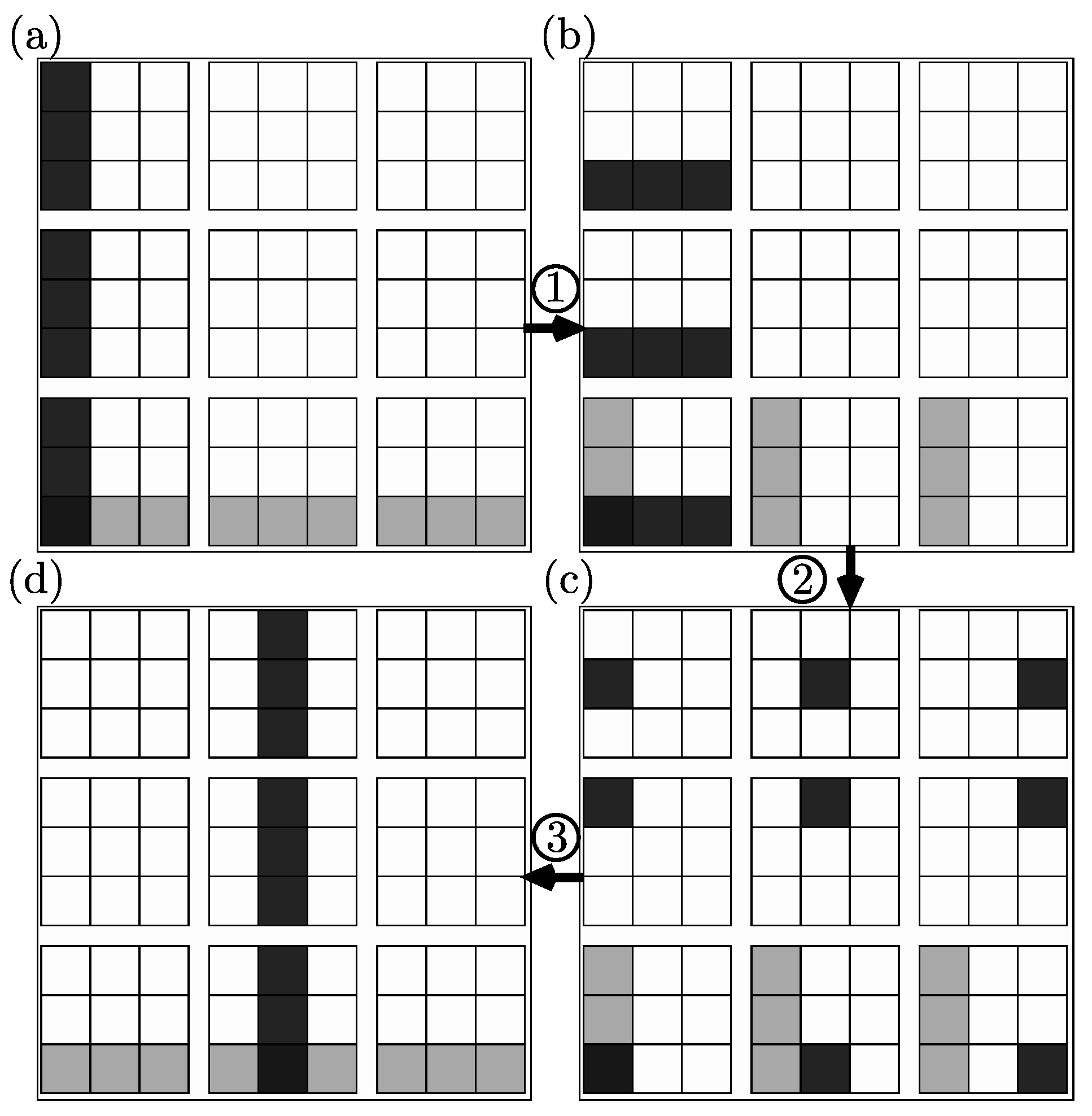
As a demonstration of what stabilizer state propagation looks like in the Wigner formalism, we proceed to go through an example of Bell state preparation and measurement starting from the state . To illustrate this process we decompose the two qutrit Wigner function of this state into nine grids, as shown in Figure 2. The prepared Wigner function is denoted in Figure 3 with the color black, and the Wigner function represented by setting (i.e., considering the top n rows of to be a separate Wigner function, as discussed at the end of Section 3.1) is denoted with the color gray.
We begin with
denoting an initially prepared state of . This is clear in Figure 3a by the black band that lies along all Weyl phase space points with and . On the other hand, the gray manifold is perpendicular to the black one, and lies along Weyl phase space points with and .
Acting on this state with produces . Applying the algorithm specified at the end of Section 3.2, we find:
Thus, the momentum of qutrit 1 is now determined and is 0 while the second qutrit is unchanged. This can be seen in Figure 3b, where the values of the non-zero Weyl phase space points are the same, while the state has rotated by in -space. A similar transformation has occurred for the perpendicular gray manifold.
Acting next with produces the Bell state , which is represented by the following Wigner function:
The entanglement between the two qutrits is evident in both of their dependence on each other’s momenta and positions, and , specified by the last two rows. Figure 3c shows that the state is still representable as lines in Weyl phase space, except they now traverse through the different planes of associated with each value of . However, if you consider the left column in Figure 3c corresponding to , you can see that the only black Weyl phase points are at . Similarly, the middle column corresponding to shows that , and the right column corresponding to shows that too, confirming that . Thus, the entanglement of the two qutrits’ positions is clearly evident in this Figure of the Wigner function.
We then proceed to measure qutrit 1. Since the lower two equations involve , we know that this is a random measurement. Let us pick the outcome to be 1 and set the third row as such, replacing the first row with the old third row. This collapses qutrit 2 into the same state:
The lower two rows show that now , as we chose, and . The collapse of qutrit 2 into can also been seen in Figure 3c by the fact that only in the grids that correspond to too.
Finally, the fact that a measurement of would be deterministic at this point can be seen in the fact that is not present in the last two rows of . Furthermore, it is clear, since the first row has a coefficient of 1 in front of , that the corresponding third row must be added with weight 1 to the fourth row to obtain this deterministic measurement outcome of . This can also be seen in Figure 3 by finding the projection of onto , which are shown by the gray manifolds in panels (a) and (d), respectively. They are collinear and so the projection is equal to 1. (Perpendicular manifolds corresponds to a projection of 0, and those that lie diagonally with respect to each other have a projection equal to 2 in this discrete geometry.)
7. Conclusions
In summary, we introduced an algorithm that efficiently simulates stabilizer state evolution under Clifford gates and measurements in the Pauli basis for odd d qudits. We accomplished this by relying on the phase-space perspective of stabilizer states as discrete Gaussians and Clifford operators as having underlying harmonic Hamiltonians. We showed the equivalence of our algorithm, through Equations (43) and (44), to the well-known Aaronson–Gottesman tableau algorithm [2] for qubits, revealing that Aaronson–Gottesman’s tableau corresponds to a discrete Wigner function. As a consequence, we revealed the physically intuitive phase space perspective of Aaronson–Gottesman’s algorithm, as well as its extension to higher odd d.
This work illustrates that no efficiency advantage is gained by using the Heisenberg representation for stabilizer propagation. Equation (44) indicates that the Heisenberg representation is equivalent to the Schrödinger representation in this context; evolving the operators is just as efficient as evolving the states, as perhaps expected.
Lastly, the correspondence between the Wigner-based algorithm and the Aaronson–Gottesman tableau algorithm may point the direction on how to resolve the long-standing issue of describing the Wigner–Weyl–Moyal and center-chord formalism for systems. We have shown that the Aaronson–Gottesman algorithm is essentially a treatment of the Wigner approach. The salient difference appears to be the state-dependence of this evolution, and likely is related to the state-independent contextuality that qubits exhibit, which odd d qudits do not. Exploring the details of this state-dependence is a promising subject of future study.
Acknowledgments
This work was supported by the Air Force Office of Scientific Research (AFOSR) award No. FA9550-12-1-0046.
Author Contributions
All authors contributed to the work presented here.
Conflicts of Interest
The authors declare no conflict of interest.
References
- Gottesman, D. The Heisenberg Representation of Quantum Computers. arXiv, 1998; arXiv:quant-ph/9807006. [Google Scholar]
- Aaronson, S.; Gottesman, D. Improved simulation of stabilizer circuits. Phys. Rev. A 2004, 70, 052328. [Google Scholar] [CrossRef]
- Gottesman, D. Fault-tolerant quantum computation with higher-dimensional systems. In Quantum Computing and Quantum Communications; Springer: Heidelberg, Germany, 1999; pp. 302–313. [Google Scholar]
- Mari, A.; Eisert, J. Positive Wigner functions render classical simulation of quantum computation efficient. Phys. Rev. Lett. 2012, 109, 230503. [Google Scholar] [CrossRef] [PubMed]
- Howard, M.; Wallman, J.; Veitch, V.; Emerson, J. Contextuality supplies the `magic’ for quantum computation. Nature 2014, 510, 351–355. [Google Scholar] [CrossRef] [PubMed]
- Wootters, W.K. A Wigner-function formulation of finite-state quantum mechanics. Ann. Phys. 1987, 176, 1–21. [Google Scholar] [CrossRef]
- Gross, D. Hudson’s theorem for finite-dimensional quantum systems. J. Math. Phys. 2006, 47, 122107. [Google Scholar] [CrossRef]
- Veitch, V.; Ferrie, C.; Gross, D.; Emerson, J. Negative quasi-probability as a resource for quantum computation. New J. Phys. 2012, 14, 113011. [Google Scholar] [CrossRef]
- Veitch, V.; Wiebe, N.; Ferrie, C.; Emerson, J. Efficient simulation scheme for a class of quantum optics experiments with non-negative Wigner representation. New J. Phys. 2013, 15, 013037. [Google Scholar] [CrossRef]
- Kocia, L.; Love, P. Semiclassical Formulation of Gottesman–Knill and Universal Quantum Computation. arXiv, 2016; arXiv:1612.05649. [Google Scholar]
- Koh, D.E.; Penney, M.D.; Spekkens, R.W. Computing quopit Clifford circuit amplitudes by the sum-over-paths technique. arXiv, 2017; arXiv:1702.03316. [Google Scholar]
- De Beaudrap, N. A linearized stabilizer formalism for systems of finite dimension. arXiv, 2011; arXiv:1102.3354. [Google Scholar]
- Yoder, T.J. A Generalization of the Stabilizer Formalism for Simulating Arbitrary Quantum Circuits. 2012. Available online: https://pdfs.semanticscholar.org/b200/efe1709d07ffc1b5b7bd90e61c09e2729bdf.pdf (accessed on 6 July 2017).
- Anders, S.; Briegel, H.J. Fast simulation of stabilizer circuits using a graph-state representation. Phys. Rev. A 2006, 73, 022334. [Google Scholar] [CrossRef]
- Bengtsson, I.; Zyczkowski, K. On discrete structures in finite Hilbert spaces. arXiv, 2017; arXiv:1701.07902. [Google Scholar]
- Mermin, N.D. Hidden variables and the two theorems of John Bell. Rev. Mod. Phys. 1993, 65, 803. [Google Scholar] [CrossRef]
- Raussendorf, R.; Browne, D.E.; Delfosse, N.; Okay, C.; Bermejo-Vega, J. Contextuality as a resource for qubit quantum computation. arXiv, 2015; arXiv:1511.08506. [Google Scholar]
- Kocia, L.; Love, P. Discrete Wigner Formalism for Qubits and the Non-Contextuality of Clifford Operations on Qubit Stabilizer States. arXiv, 2017; arXiv:1705.08869. [Google Scholar]
Figure 1.
The initial perpendicular manifolds and and the harmonically evolved perpendicular manifolds and . Description of the various lengths and angles are given in the text in the proof of Lemma 1.
Figure 1.
The initial perpendicular manifolds and and the harmonically evolved perpendicular manifolds and . Description of the various lengths and angles are given in the text in the proof of Lemma 1.
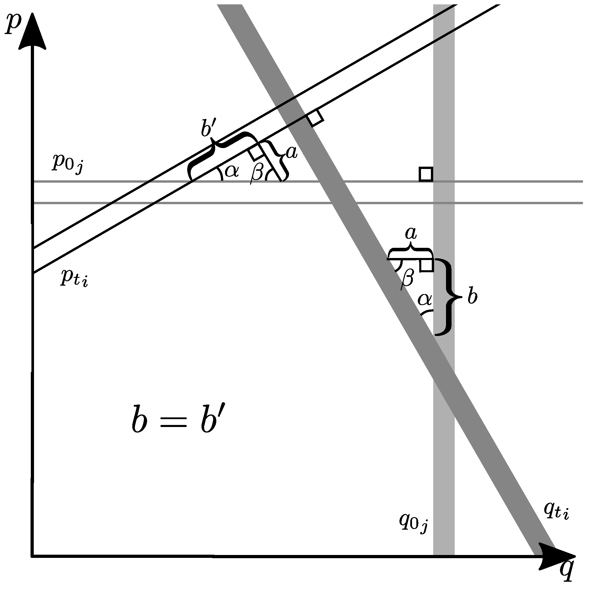
Figure 2.
A decomposition of the two qutrit Wigner function into nine grids, where each grid denotes the value of the Wigner function at all and for a fixed value of and denoted by the external axes. This organization is used in Figure 3 below.
Figure 2.
A decomposition of the two qutrit Wigner function into nine grids, where each grid denotes the value of the Wigner function at all and for a fixed value of and denoted by the external axes. This organization is used in Figure 3 below.
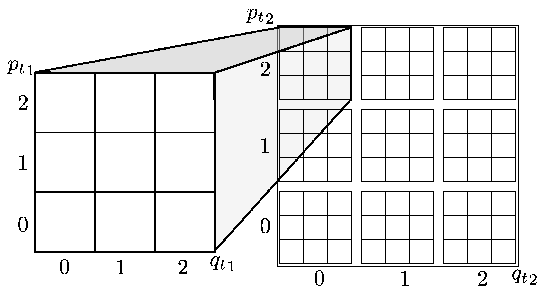
Figure 3.
The Wigner function of two qutrits initially prepared in (a) the state . (1) This is evolved under to produce (b) . (2) Subsequently, this state is evolved under producing (c) the Bell state . (3) Qutrit 1 is then measured producing the random outcome 1, which collapses qutrit 2 into the same state, so that (d) results. The black color indicates the Wigner function specified by the lowest n rows of , and the gray color indicates the Wigner function specified by the highest n rows ( and , respectively). The evolution and algorithmic implementation are explained in the text.

Table 1.
Transformation of stabilizer generators under Clifford operations.
| Gates | Input | Output |
|---|---|---|
| Hadamard | ||
| phase | ||
| CNOT | ||
Table 2.
Binary representation of the Pauli operators and the Pauli group phase used in their tableau representation.
Table 2.
Binary representation of the Pauli operators and the Pauli group phase used in their tableau representation.
| 0 | 0 | |
| 0 | 1 | |
| 1 | 0 | |
| 1 | 1 | |
| Phase | ||
| 0 | ||
| 1 |
© 2017 by the authors. Licensee MDPI, Basel, Switzerland. This article is an open access article distributed under the terms and conditions of the Creative Commons Attribution (CC BY) license (http://creativecommons.org/licenses/by/4.0/).
Share and Cite
MDPI and ACS Style
Kocia, L.; Huang, Y.; Love, P. Discrete Wigner Function Derivation of the Aaronson–Gottesman Tableau Algorithm. Entropy 2017, 19, 353. https://doi.org/10.3390/e19070353
AMA Style
Kocia L, Huang Y, Love P. Discrete Wigner Function Derivation of the Aaronson–Gottesman Tableau Algorithm. Entropy. 2017; 19(7):353. https://doi.org/10.3390/e19070353
Chicago/Turabian StyleKocia, Lucas, Yifei Huang, and Peter Love. 2017. "Discrete Wigner Function Derivation of the Aaronson–Gottesman Tableau Algorithm" Entropy 19, no. 7: 353. https://doi.org/10.3390/e19070353
Note that from the first issue of 2016, this journal uses article numbers instead of page numbers. See further details here.