Study on the Business Cycle Model with Fractional-Order Time Delay under Random Excitation

1
Department of Applied Mathematics, Northwestern Polytechnical University, Xi’an 710072, China
2
School of Statistics, Xi’an University of Finance & Economics, Xi’an 710061, China
*
Author to whom correspondence should be addressed.
Entropy 2017, 19(7), 354; https://doi.org/10.3390/e19070354
Submission received: 31 May 2017
/
Revised: 2 July 2017
/
Accepted: 10 July 2017
/
Published: 12 July 2017
(This article belongs to the Special Issue Complex Systems, Non-Equilibrium Dynamics and Self-Organisation)
Abstract
:Time delay of economic policy and memory property in a real economy system is omnipresent and inevitable. In this paper, a business cycle model with fractional-order time delay which describes the delay and memory property of economic control is investigated. Stochastic averaging method is applied to obtain the approximate analytical solution. Numerical simulations are done to verify the method. The effects of the fractional order, time delay, economic control and random excitation on the amplitude of the economy system are investigated. The results show that time delay, fractional order and intensity of random excitation can all magnify the amplitude and increase the volatility of the economy system.
1. Introduction
The business cycle model is one of the most attractive models in applying the concept of nonlinear dynamic to investigate economic phenomenon [1]. Many scholars have been working on this model. Li et al. [2] studied chaos prediction and chaos control of the model under random excitation. Li et al. [3] investigated the first-passage failure of a business cycle model under wide-brand random excitation. Time delay in a real economy system is ubiquitous. When a policy decision is made, requires some time to implement the economic policy. Yoshida and Asada [4] investigated the effect of policy lag on macroeconomic stability and revealed that policy lag contributed to chaotic motion. Ma et al. [5] studied the stability of the equilibrium and the existence of Hopf bifurcations of business cycle model with discrete delay. Wu et al. [6] investigated the multi-parameter bifurcations of the Kaldor–Kalecki model of business cycles with delay. Khalid Hattaf et al. [7,8] investigated a delayed business cycle model with general investment function. Liu et al. [9] investigated the stability and Hopf bifurcation for a business cycle model with expectation and time delay. Li et al. [10] investigated the stochastic response of business cycle model with time-delay feedback.
When analyzing the time series, the series often present autocorrelation. How to describe this property in a continuous model is undefined. In recent years, a lot of work has been done on the issue of fractional calculus [11,12,13,14,15,16,17,18,19,20,21]. In the research of fractional-order delay, Shen et al. [22,23] investigated the dynamical response of Mathieu–Duffing oscillator with fractional-order delayed feedback and analyzed the Duffing oscillator with time-delayed fractional-order Proportion, Integration, Differentiation (PID) controller. In the field of economic and finance modeling, many papers on fractional modeling are published. Nick Laskin [24] investigated the equation of financial assets with fractional derivative and studied the probability distribution function (pdf) of the returns. Yin et al. [25] designed a sliding-mode control law to control chaos in a class of fractional-order chaotic systems. The fractional-order financial system is also investigated by some scholars [26,27,28,29].
Stochastic perturbations are omnipresent and inevitable in an economy system. These random factors can also influence the dynamics of the economy system. Spanos et al. [30] presented a frequency-domain method to investigate the stochastic systems with fractional derivatives. Chen and Zhu et al. [31,32,33,34,35,36] have applied stochastic averaging method to complete a lot of excellent work on the nonlinear systems with fractional derivatives. Huang and Jin et al. [37] studied the response and stability of a strongly nonlinear stochastic system with light fractional damping. Hu and Zhu et al. [38] investigated stochastic fractional optimal control of quasi-integrable Hamiltonian system with fractional derivative damping. Xu and Li et al. [39,40] put forward a new Lindstedt–Poincare method to obtain the approximate solution of fractional oscillators under random excitation. Liu [41] studied the principal resonance responses of single-degree-of-freedom systems with small fractional derivative damping under the narrow-band random parametric excitation by multiple scales method. Lin et al. [42] investigated the business cycle model with fractional derivative under narrow-band random excitation.
This paper is organized as follows. In Section 2, considering the memory property of economic policy making, and the delay of implementing the economic policy, we present a mathematical model of a business cycle model with fractional time delay under random excitation based on Goodwin’s model. In Section 3, we applied stochastic averaging method to obtain the approximate analytical solution. In Section 4, we do simulations to verify the theoretical results and investigate the effects of fractional-order derivative, time delay, random excitation and economic control on the amplitude of economy system.
2. The Model
In the literature [1], Goodwin considered the lag between decisions to invest and the corresponding outlays that tend to lag behind decisions. Therefore, we may say
where is the national income, the marginal propensity to consume, the investment delay, the construction time of new equipment, the function of decisions to invest, the autonomous outlays. It is actually the equation that income equals consumption and investment.
By Taylor expansion and dropping all but the first two terms in each, we can obtain
To eliminate , we set
Equation (2) can be written as
With some transformations, Equation (3) can be written as
where
the model can be written as
where
Considering economic control to control the economic fluctuation, Equation (7) can be written as
where denotes economic control.
Also, considering time delay and memory property of implementing economic policy and random excitation, Equation (8) can be written as
where denotes the fractional-order time-delay economic control.
3. Stationary PDF of the Model with Random Excitation
In this section, we will apply the stochastic averaging method to obtain the approximate solution of the amplitude of the economy system (9). If the intensity of the noise , the response of system (9) is a stochastic process which is non-Markovian due to the fractional-order time delay. In this section, approximate method has been applied to obtain the stationary PDF for the amplitude of the response.
Stochastic Averaging Method
Equation (9) can be regarded as random spread of periodic motion of the linear differential equation.
We set , the solution can be assumed as
By differentiating Equation (11a) to , we can obtain
By differentiating Equation (11b) to , we can obtain
Substituting Equations (11) and (13) into Equation (9), we can obtain
So, we can obtain the following equation
Applying stochastic averaging method to Equation (15) in time interval [0 T], we can obtain the approximation of the amplitude and the phase as
is periodic function and we set . is aperiodic and we set , and we can obtain the first part of Equation (16)
So, the second part of Equation (16) can be written as
In Equation (17), we applied Caputo’s definition and the expression is as follows
where is the fractional-order derivative
With the transformation and , Equation (20) can be written
With two basic formulas, we can obtain
Similarly, we can also obtain
Thus, combining with Equation (17), we can obtain
where , are independent normalized sources of Gaussian white noise. Then the averaged Itô equation for is the following form:
where
So, we can obtain the Fokker–Planck–Kolmogrov (FPK) equation of amplitude
and the stationary solution of system (9) is
where is the normalization constant and .
4. Nonlinear Investment Function
In this section, we set . is the reciprocal of an adjustment coefficient. This means that the induced investment is a cubic nonlinear function. Substituting this formula into Equation (9), Equation (9) can be written as follows
Based on the analysis in Section 3, we can obtain the averaged Itô equation for the amplitude
The stationary solution of the system (30) is
where is the normalization constant.
4.1. The Effect of Fractional-Order Time Delay
Firstly, we investigate the effect of time delay on the amplitude of the economy system. We set and , then system (29) is a deterministic system. From Figure 1, we can obtain that the fractional time delay can change the stability of the fixed point. When in Figure 1a,c, the fixed point is asymptotical stability. When in Figure 1b,d, a limit cycle can be obtained. In other words, when the effect of fractional time delay exists, the economy system will still have periodic fluctuations even it is under economic control. It means that the economic control is ineffective. So, the policy maker must consider this when making economic control.
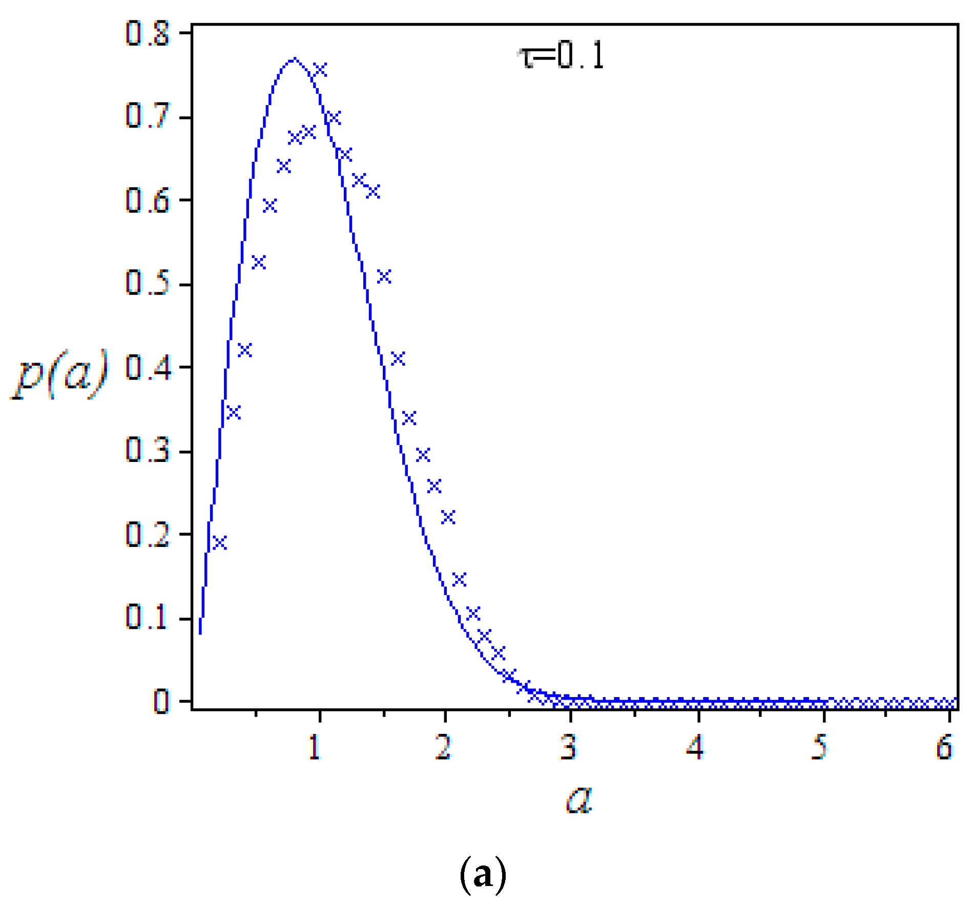
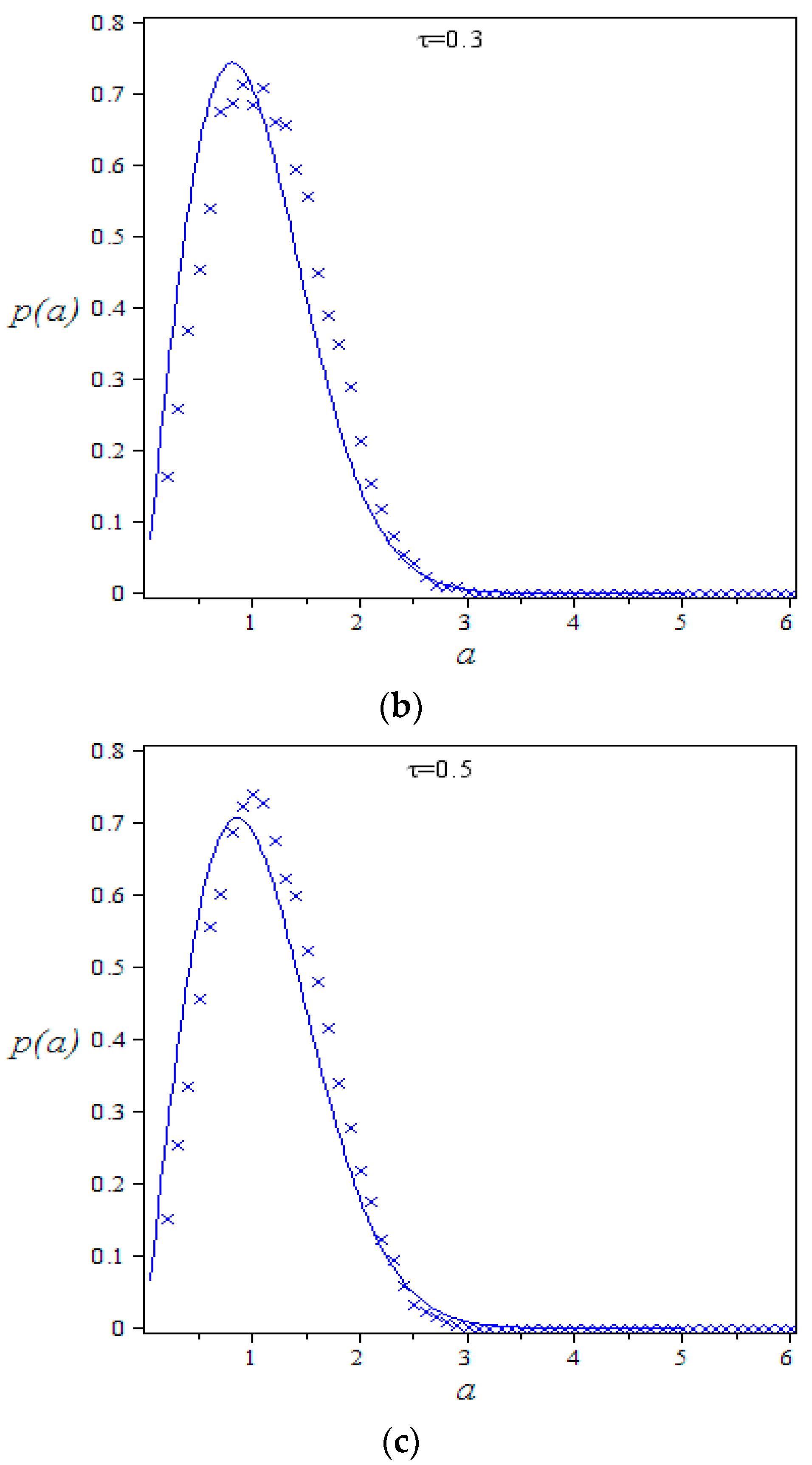
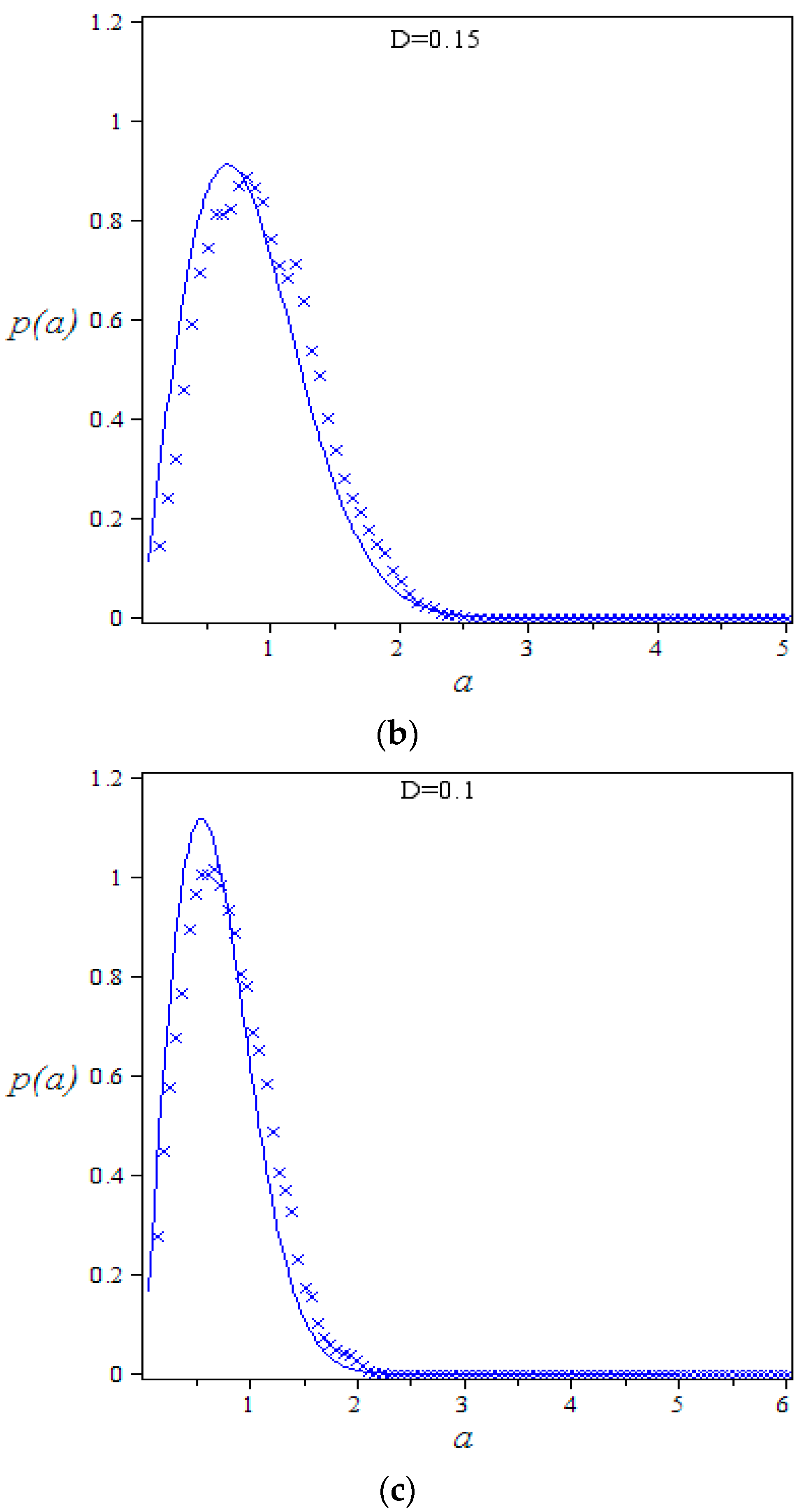
When we consider the stochastic situation. Figure 2 is the stationary probability density of amplitude for different values of time delay. We can obtain the numerical solutions and the analytical solutions are in good agreement. Thus, it can prove the validity of the method proposed in this paper. The peak of stationary probability density function represents the stability of the economy system. The higher peak indicates the stronger stability. In Figure 2, the peak is decreasing with the increase of time delay. This means that time delay lowers the stability of the economy system. With the increase of time delay the amplitude on its peak of stationary probability density function of the economy system is magnified. This means that the time delay can magnify the amplitude of the economy system. By Equation (31), we obtain the stationary probability density function related to time delay . Thus, the policy maker can evaluate the effect of time delay of implementing economic policy to put the economy under control.
4.2. The Effect of the Fractional-Order
In this section, we study the effect of fractional order on the amplitude of the economy system (28). Figure 3 is the stationary probability density of amplitude for different values of fractional order. From Figure 3, we can obtain that the peak is decreasing with the decrease of the fractional-order derivative. In other words, with the increase of the fractional-order derivative, the stability of the economy system is magnified. The smaller fractional-order derivative represents the stronger memory effect of economic control. This means that the memory property can lower the stability of the economy system. On the other hand, the smaller fractional-order derivative has a bigger amplitude on its peak of stationary probability density function. This means that the memory property of economic control can magnify the amplitude of the economy system. This indicates that the memory property of economic control actually plays a negative role in making the economy system under control, and we can compute the effect of memory property by Equation (31). So the policy maker can make effective economic policy to make the economy under control.
4.3. The Effect of Economic Control
Figure 4 is the stationary probability density of amplitude for different values of intensity of economic control. The peak is decreasing with the decrease of the intensity of economic control. This means that the economic control improves the stability of the economy system. With the decrease of economic control, the amplitude on its peak of stationary probability density function of the economy system is magnified. This means that the economic control lowers the amplitude of the economy system, and we can compute the effect of economic control by Equation (31). It is helpful to the policy maker to make economic policy to make the economy under control.
4.4. The Effect of Random Excitation
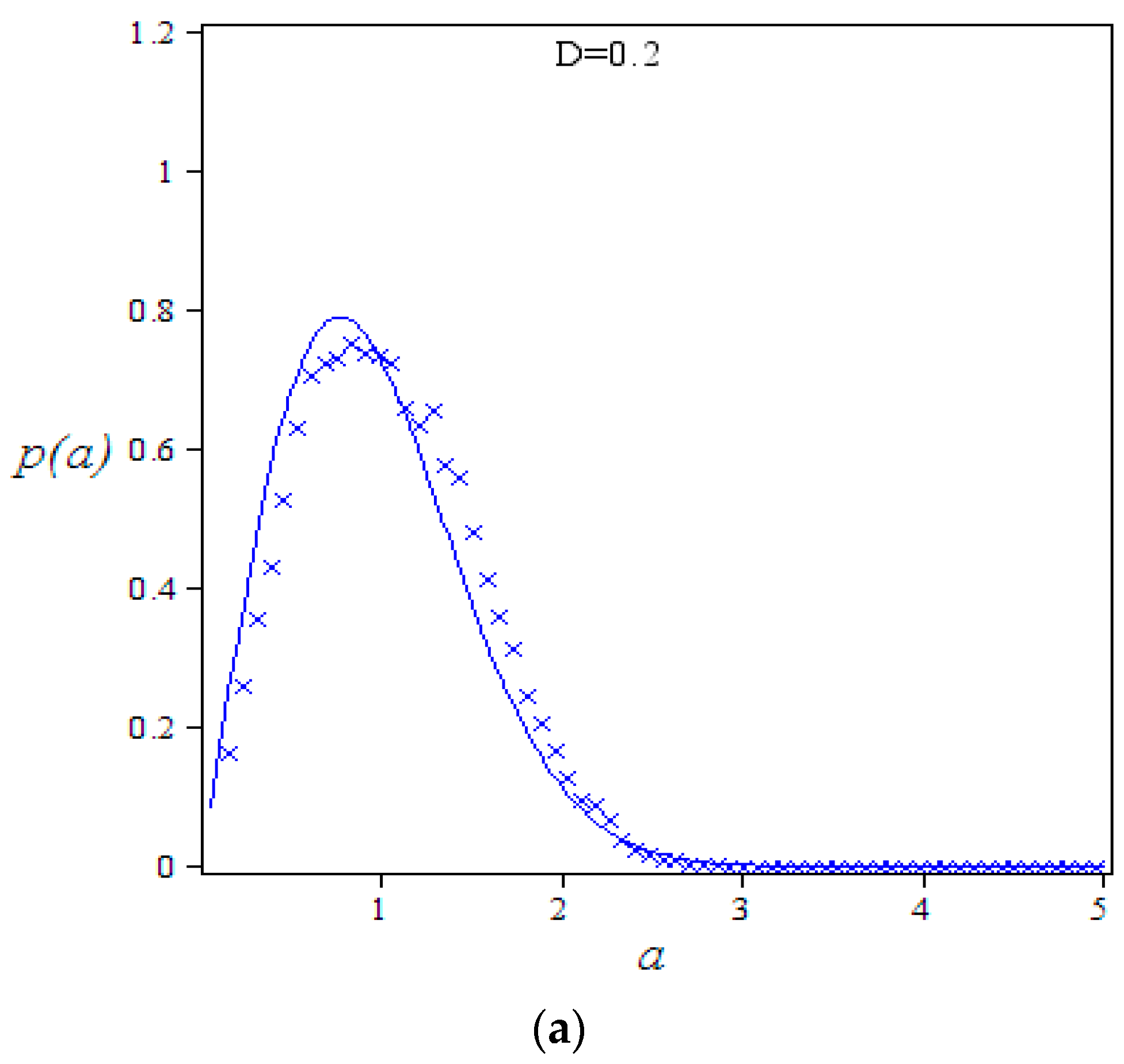
Figure 5 is the stationary probability density of amplitude for different values of intensity of random excitation. The peak is decreasing with the increase of the intensity of random excitation. This means that the external random excitation lowers the stability of the economy system. With the increase of the intensity of random excitation, the amplitude on its peak of stationary probability density function of the economy system is magnified. This means that external random excitation can magnify the amplitude of the economy system, and we can compute the effect of random excitation by Equation (31). It is helpful to the policy maker to make economic policy to make the economy under control.
5. Conclusions
In this paper, we investigate the stochastic response of a business cycle model with fractional-order time delay under random excitation. We applied stochastic averaging method to obtain the approximate analytical solution. Thus, we can get the accurate solution of the stationary probability density function. The effect of fractional time delay on the stability and amplitude of the economy system is investigated. The results show that the time delay can induce the Hopf bifurcation in a deterministic model and lower the stability of the economy system in the stochastic situation, and the amplitude of the economy system is magnified by time delay. Also, the effect of fractional order on the stationary probability density function is studied. The results show that the memory property of economic control lowers the stability and magnifies the amplitude of the economy system. Then, the effect of intensity of economic control is investigated. The results show that strengthened economic control can improve the stability and lower the amplitude of the economy system. Finally, the influence of external random excitation on the stationary probability density function is researched. The results indicate that the stronger external random excitation brings a bigger amplitude and lower stability of the economy system. The analysis above is helpful to the policy maker to make economic policy to make the economy under control.
Acknowledgments
The authors thank the reviewer for the careful reading and suggestions. The research was supported by the National Natural Science Foundation of China (Grant NOs. 11532011, 11572231, 11502199, 11672233).
Author Contributions
Zifei Lin, Wei Xu and Jiaorui Li collectively realized theoretical analyses; Wantao Jia and Shuang Li computed the numerical simulation results; Zifei Lin wrote the paper. All authors have read and approved the final manuscript.
Conflicts of Interest
The authors declare no conflict of interest.
References
- Goodwin, R.M. The nonlinear accelerator and the persistence of business cycles. Econom. J. Econom. Soc. 1951, 19, 1–17. [Google Scholar] [CrossRef]
- Li, S.; Li, Q.; Li, J.; Feng, J. Chaos prediction and control of Goodwin’s nonlinear accelerator model. Nonlinear Anal. Real World Appl. 2011, 12, 1950–1960. [Google Scholar] [CrossRef]
- Li, J.; Feng, C.S. First-passage failure of a business cycle model under time-delayed feedback control and wide-band random excitation. Phys. A Stat. Mech. Appl. 2010, 389, 5557–5562. [Google Scholar] [CrossRef]
- Yoshida, H.; Asada, T. Dynamic analysis of policy lag in a Keynes–Goodwin model: Stability, instability, cycles and chaos. J. Econ. Behav. Org. 2007, 62, 441–469. [Google Scholar] [CrossRef]
- Ma, J.; Gao, Q. Stability and Hopf bifurcations in a business cycle model with delay. Appl. Math. Comput. 2009, 215, 829–834. [Google Scholar] [CrossRef]
- Wu, X.P.; Wang, L. Multi-parameter bifurcations of the Kaldor–Kalecki model of business cycles with delay. Nonlinear Anal. Real World Appl. 2010, 11, 869–887. [Google Scholar] [CrossRef]
- Hattaf, K.; Riad, D.; Yousfi, N. A generalized business cycle model with delays in gross product and capital stock. Chaos Solitons Fractals 2017, 98, 31–37. [Google Scholar] [CrossRef]
- Riad, D.; Hattaf, K.; Yousfi, N. Dynamics of a delayed business cycle model with general investment function. Chaos Solitons Fractals 2016, 85, 110–119. [Google Scholar] [CrossRef]
- Liu, X.; Cai, W.; Lu, J.; Wang, Y. Stability and Hopf bifurcation for a business cycle model with expectation and delay. Commun. Nonlinear Sci. Numer. Simul. 2015, 25, 149–161. [Google Scholar] [CrossRef]
- Li, J.; Ren, Z.; Wang, Z. Response of nonlinear random business cycle model with time delay state feedback. Phys. A Stat. Mech. Appl. 2008, 387, 5844–5851. [Google Scholar] [CrossRef]
- Bagley, R.L.; Torvik, J. Fractional calculus—A different approach to the analysis of viscoelastically damped structures. AIAA J. 1983, 21, 741–748. [Google Scholar] [CrossRef]
- Bagley, R.L.; Torvik, P. A theoretical basis for the application of fractional calculus to viscoelasticity. J. Rheol. 1983, 27, 201–210. [Google Scholar] [CrossRef]
- Bagley, R.L.; Torvik, P.J. Fractional calculus in the transient analysis of viscoelastically damped structures. AIAA J. 1985, 23, 918–925. [Google Scholar] [CrossRef]
- Caputo, M.; Mainardi, F. A new dissipation model based on memory mechanism. Pure Appl. Geophys. 1971, 91, 134–147. [Google Scholar] [CrossRef]
- Kelly, J.M.; Koh, C. Application of fractional derivatives to seismic analysis of base isolated models. Earthq. Eng. Struct. Dyn. 1990, 19, 229–241. [Google Scholar]
- Rossikhin, Y.A.; Shitikova, M.V. Applications of fractional calculus to dynamic problems of linear and nonlinear hereditary mechanics of solids. Appl. Mech. Rev. 1997, 50, 15–67. [Google Scholar] [CrossRef]
- Rossikhin, Y.A.; Shitikova, M.V. Application of fractional calculus for dynamic problems of solid mechanics: Novel trends and recent results. Appl. Mech. Rev. 2010, 63, 010801. [Google Scholar] [CrossRef]
- Gemant, A. XLV. On fractional differentials. Lond. Edinb. Dublin Philos. Mag. J. Sci. 1938, 25, 540–549. [Google Scholar] [CrossRef]
- Pritz, T. Analysis of four-parameter fractional derivative model of real solid materials. J. Sound Vib. 1996, 195, 103–115. [Google Scholar] [CrossRef]
- Diethelm, K.; Ford, N.J.; Freed, A.D. A predictor-corrector approach for the numerical solution of fractional differential equations. Nonlinear Dyn. 2002, 29, 3–22. [Google Scholar] [CrossRef]
- Podlubny, I. Mathematics in Science and Engineering. In Fractional Differential Equations; Academic Press: Cambridge, MA, USA, 1999. [Google Scholar]
- Shen, Y.; Yang, S.; Xing, H.; Gao, G. Primary resonance of Duffing oscillator with fractional-order derivative. Commun. Nonlinear Sci. Numer. Simul. 2012, 17, 3092–3100. [Google Scholar] [CrossRef]
- Niu, J.; Shen, Y.; Yang, S.; Li, S. Analysis of Duffing oscillator with time-delayed fractional-order PID controller. Int. J. Non-Linear Mech. 2017, 92, 66–75. [Google Scholar] [CrossRef]
- Laskin, N. Fractional market dynamics. Phys. A Stat. Mech. Appl. 2000, 287, 482–492. [Google Scholar] [CrossRef]
- Yin, C.; Zhong, S.-M.; Chen, W.-F. Design of sliding mode controller for a class of fractional-order chaotic systems. Commun. Nonlinear Sci. Numer. Simul. 2012, 17, 356–366. [Google Scholar] [CrossRef]
- Chen, W.-C. Nonlinear dynamics and chaos in a fractional-order financial system. Chaos Solitons Fractals 2008, 36, 1305–1314. [Google Scholar] [CrossRef]
- Wang, Z.; Huang, X.; Shi, G. Analysis of nonlinear dynamics and chaos in a fractional order financial system with time delay. Comput. Math. Appl. 2011, 62, 1531–1539. [Google Scholar] [CrossRef]
- Pan, I.; Das, S.; Das, S. Multi-objective active control policy design for commensurate and incommensurate fractional order chaotic financial systems. Appl. Math. Model. 2015, 39, 500–514. [Google Scholar] [CrossRef]
- Danca, M.-F.; Garrappa, R.; Tang, W.K.; Chen, G. Sustaining stable dynamics of a fractional-order chaotic financial system by parameter switching. Comput. Math. Appl. 2013, 66, 702–716. [Google Scholar] [CrossRef]
- Spanos, P.; Zeldin, B. Random vibration of systems with frequency-dependent parameters or fractional derivatives. J. Eng. Mech. 1997, 123, 290–292. [Google Scholar] [CrossRef]
- Chen, L.; Wang, W.; Li, Z.; Zhu, W. Stationary response of Duffing oscillator with hardening stiffness and fractional derivative. Int. J. Non-Linear Mech. 2013, 48, 44–50. [Google Scholar] [CrossRef]
- Chen, L.; Zhu, W. Stochastic jump and bifurcation of Duffing oscillator with fractional derivative damping under combined harmonic and white noise excitations. Int. J. Non-Linear Mech. 2011, 46, 1324–1329. [Google Scholar] [CrossRef]
- Chen, L.C.; Zhu, W.Q. Stochastic stability of Duffing oscillator with fractional derivative damping under combined harmonic and white noise parametric excitations. Acta Mech. 2009, 207, 109–120. [Google Scholar] [CrossRef]
- Chen, L.; Zhu, W. First passage failure of SDOF nonlinear oscillator with lightly fractional derivative damping under real noise excitations. Probab. Eng. Mech. 2011, 26, 208–214. [Google Scholar] [CrossRef]
- Chen, L.; Li, Z.; Zhuang, Q.; Zhu, W. First-passage failure of single-degree-of-freedom nonlinear oscillators with fractional derivative. J. Vib. Control 2013, 19, 2154–2163. [Google Scholar] [CrossRef]
- Chen, L.; Hu, F.; Zhu, W. Stochastic dynamics and fractional optimal control of quasi integrable Hamiltonian systems with fractional derivative damping. Fract. Calc. Appl. Anal. 2013, 16, 189–225. [Google Scholar] [CrossRef]
- Huang, Z.L.; Jin, X.L. Response and stability of a SDOF strongly nonlinear stochastic system with light damping modeled by a fractional derivative. J. Sound Vib. 2009, 319, 1121–1135. [Google Scholar] [CrossRef]
- Hu, F.; Zhu, W.Q.; Chen, L.C. Stochastic fractional optimal control of quasi-integrable Hamiltonian system with fractional derivative damping. Nonlinear Dyn. 2012, 70, 1459–1472. [Google Scholar] [CrossRef]
- Xu, Y.; Li, Y.; Liu, D. Response of Fractional Oscillators With Viscoelastic Term Under Random Excitation. J. Comput. Nonlinear Dyn. 2014, 9, 031015. [Google Scholar] [CrossRef]
- Xu, Y.; Li, Y.; Liu, D. A method to stochastic dynamical systems with strong nonlinearity and fractional damping. Nonlinear Dyn. 2016, 83, 2311–2321. [Google Scholar] [CrossRef]
- Liu, D.; Li, J.; Xu, Y. Principal resonance responses of SDOF systems with small fractional derivative damping under narrow-band random parametric excitation. Commun. Nonlinear Sci. Numer. Simul. 2014, 19, 3642–3652. [Google Scholar] [CrossRef]
- Lin, Z.; Li, J.; Li, S. On a business cycle model with fractional derivative under narrow-band random excitation. Chaos Solitons Fractals 2016, 87, 61–70. [Google Scholar] [CrossRef]
Figure 1.
, , , (a) Phase diagram: ; (b) Time history: ; (c) Phase diagram: ; (d) Time history: .
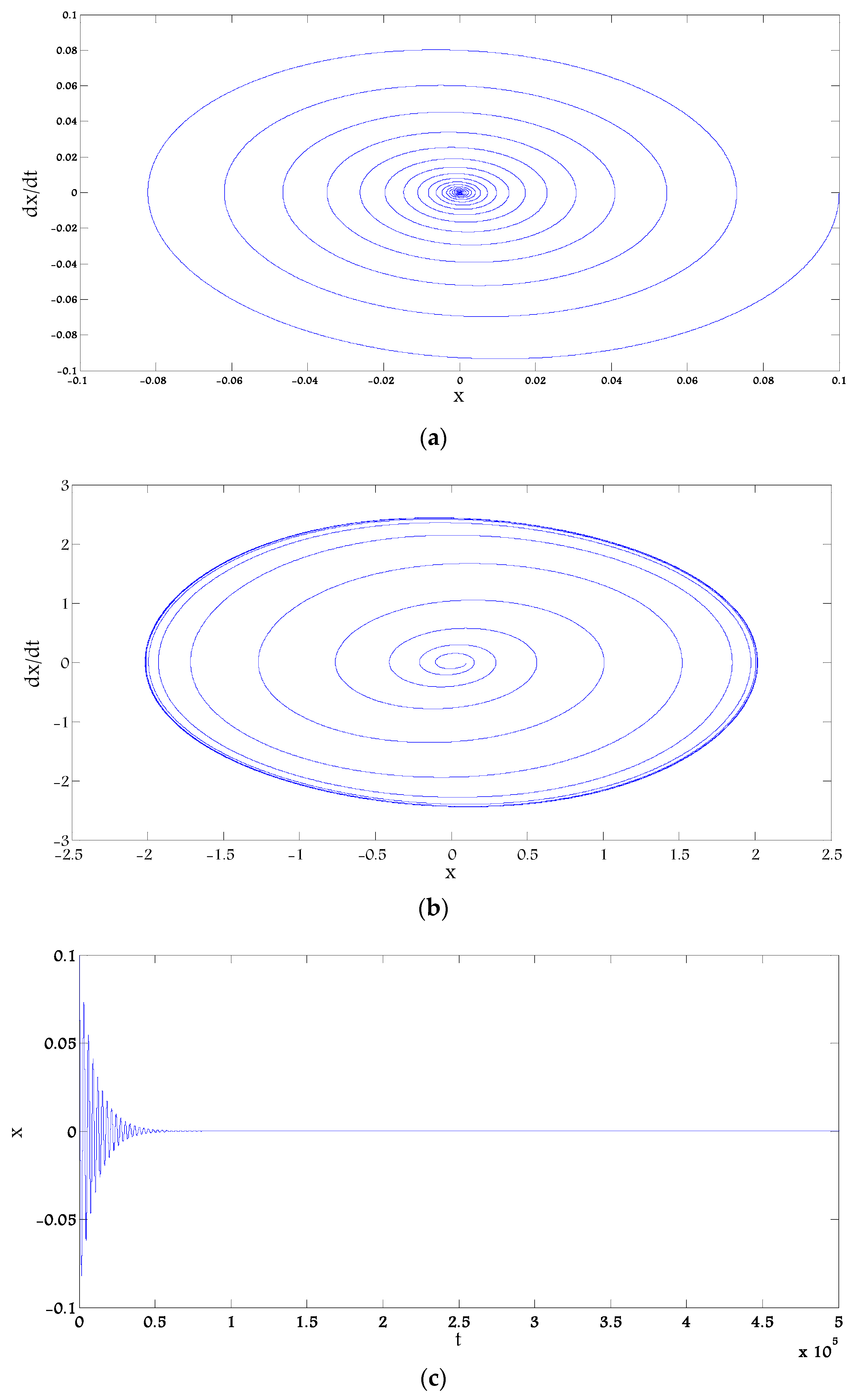
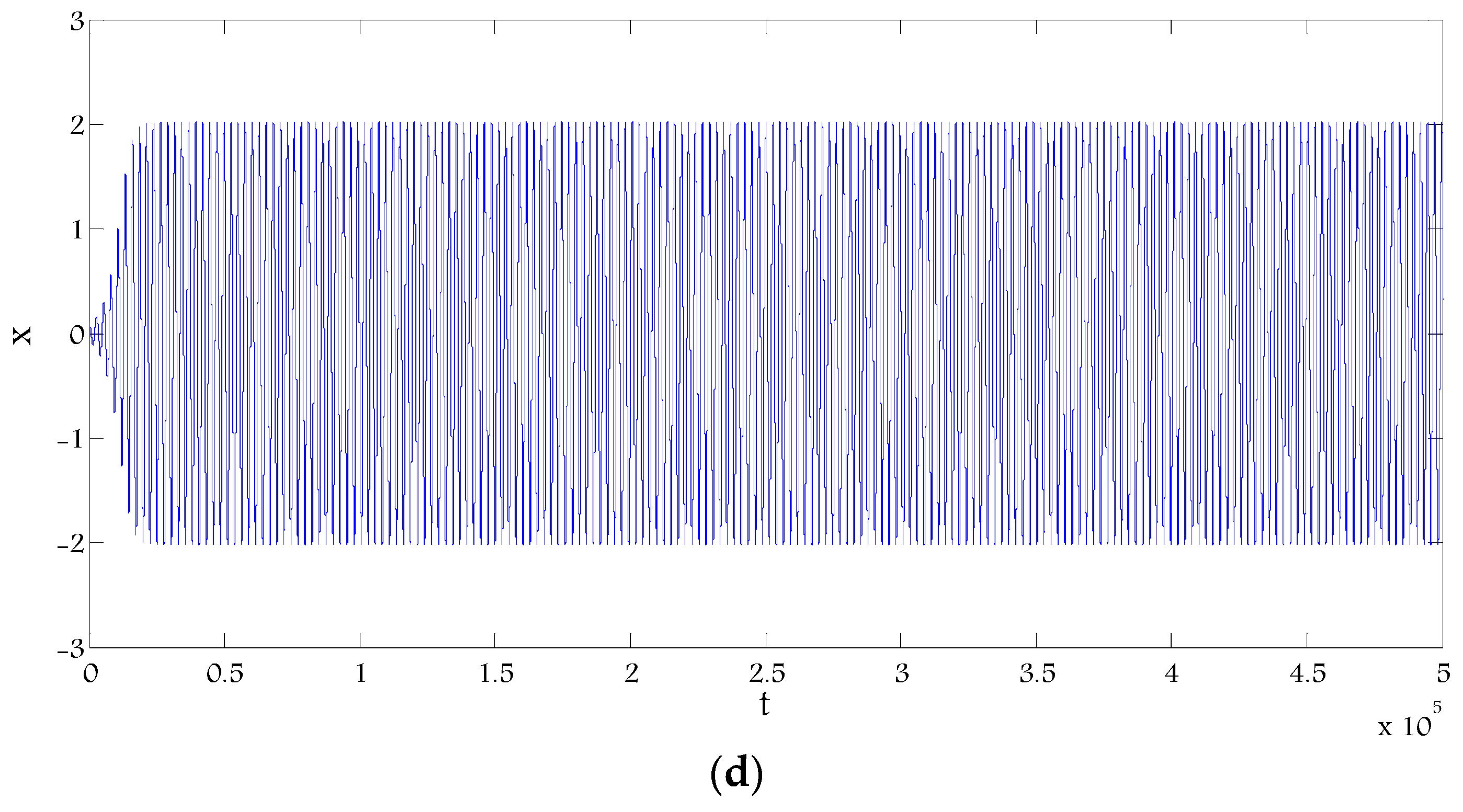
Figure 2.
The solid line “-” is analytical solutions, the crosses “x” are numerical solutions; , , , , . (a) Stationary probability density function: ; (b) Stationary probability density function: ; (c) Stationary probability density function: .
Figure 2.
The solid line “-” is analytical solutions, the crosses “x” are numerical solutions; , , , , . (a) Stationary probability density function: ; (b) Stationary probability density function: ; (c) Stationary probability density function: .


Figure 3.
The solid line “-” is analytical solutions, the crosses “x” are numerical solutions; , , , , . (a) Stationary probability density function: ; (b) Stationary probability density function: ; (c) Stationary probability density function: .
Figure 3.
The solid line “-” is analytical solutions, the crosses “x” are numerical solutions; , , , , . (a) Stationary probability density function: ; (b) Stationary probability density function: ; (c) Stationary probability density function: .
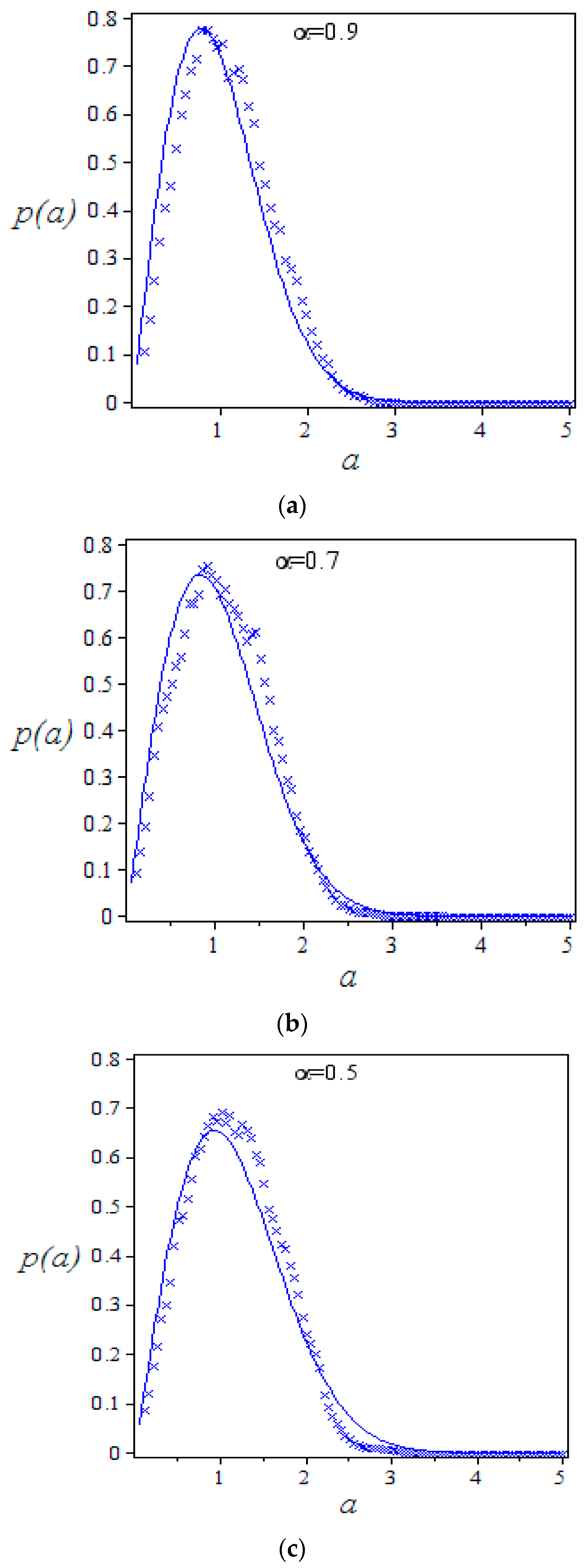
Figure 4.
The solid line “-” is analytical solutions, the crosses “x” are numerical solutions; , , , ; (a) Stationary probability density function: ; (b) Stationary probability density function: ; (c) Stationary probability density function: .
Figure 4.
The solid line “-” is analytical solutions, the crosses “x” are numerical solutions; , , , ; (a) Stationary probability density function: ; (b) Stationary probability density function: ; (c) Stationary probability density function: .
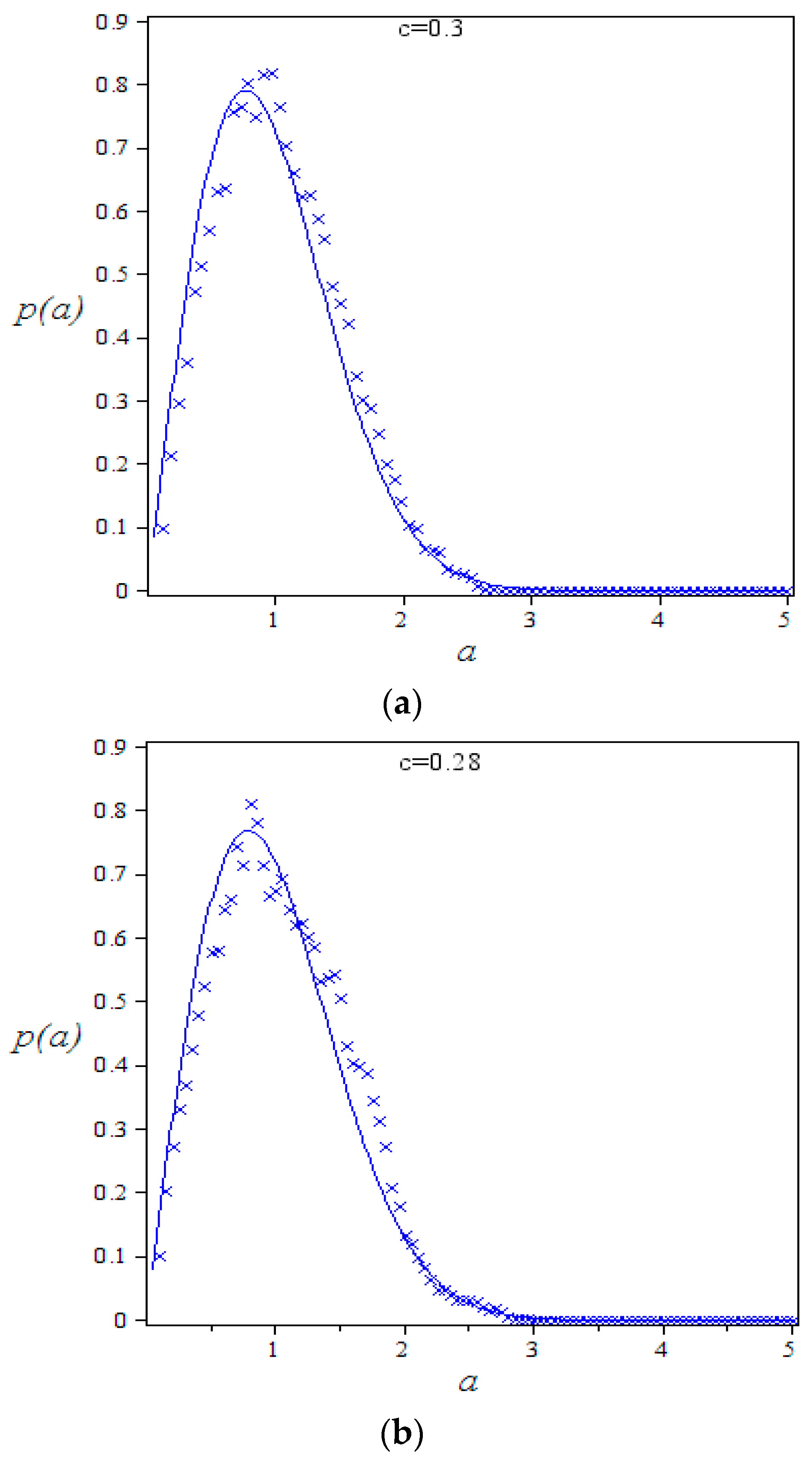
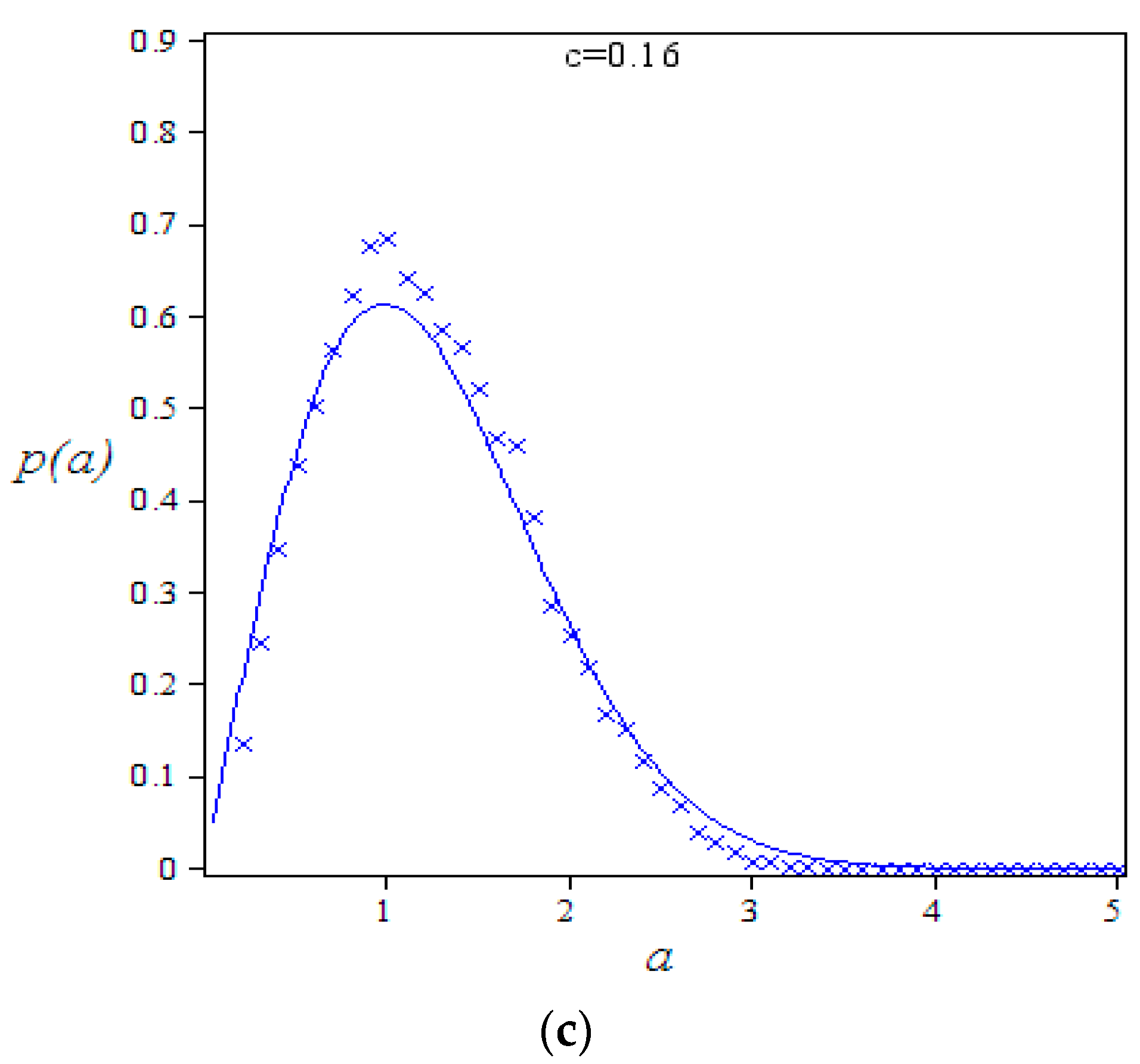
Figure 5.
The solid line “-” is analytical solutions, the crosses “x” are numerical solutions; , , , ; (a) Stationary probability density function: ; (b) Stationary probability density function: ; (c) Stationary probability density function: .
Figure 5.
The solid line “-” is analytical solutions, the crosses “x” are numerical solutions; , , , ; (a) Stationary probability density function: ; (b) Stationary probability density function: ; (c) Stationary probability density function: .
© 2017 by the authors. Licensee MDPI, Basel, Switzerland. This article is an open access article distributed under the terms and conditions of the Creative Commons Attribution (CC BY) license (http://creativecommons.org/licenses/by/4.0/).
Share and Cite
MDPI and ACS Style
Lin, Z.; Xu, W.; Li, J.; Jia, W.; Li, S. Study on the Business Cycle Model with Fractional-Order Time Delay under Random Excitation. Entropy 2017, 19, 354. https://doi.org/10.3390/e19070354
AMA Style
Lin Z, Xu W, Li J, Jia W, Li S. Study on the Business Cycle Model with Fractional-Order Time Delay under Random Excitation. Entropy. 2017; 19(7):354. https://doi.org/10.3390/e19070354
Chicago/Turabian StyleLin, Zifei, Wei Xu, Jiaorui Li, Wantao Jia, and Shuang Li. 2017. "Study on the Business Cycle Model with Fractional-Order Time Delay under Random Excitation" Entropy 19, no. 7: 354. https://doi.org/10.3390/e19070354
Note that from the first issue of 2016, this journal uses article numbers instead of page numbers. See further details here.