Extracting Knowledge from the Geometric Shape of Social Network Data Using Topological Data Analysis


1
Computer Science and Engineering Department, University of Bridgeport, Bridgeport, CT 06614, USA
2
ASML, 77 Danbury RD, Wilton, CT 06897, USA
*
Author to whom correspondence should be addressed.
Entropy 2017, 19(7), 360; https://doi.org/10.3390/e19070360
Submission received: 13 May 2017
/
Revised: 10 July 2017
/
Accepted: 14 July 2017
/
Published: 14 July 2017
(This article belongs to the Special Issue Information Geometry II)
Abstract
:Topological data analysis is a noble approach to extract meaningful information from high-dimensional data and is robust to noise. It is based on topology, which aims to study the geometric shape of data. In order to apply topological data analysis, an algorithm called mapper is adopted. The output from mapper is a simplicial complex that represents a set of connected clusters of data points. In this paper, we explore the feasibility of topological data analysis for mining social network data by addressing the problem of image popularity. We randomly crawl images from Instagram and analyze the effects of social context and image content on an image’s popularity using mapper. Mapper clusters the images using each feature, and the ratio of popularity in each cluster is computed to determine the clusters with a high or low possibility of popularity. Then, the popularity of images are predicted to evaluate the accuracy of topological data analysis. This approach is further compared with traditional clustering algorithms, including k-means and hierarchical clustering, in terms of accuracy, and the results show that topological data analysis outperforms the others. Moreover, topological data analysis provides meaningful information based on the connectivity between the clusters.
1. Introduction
These days, social networks have attracted billions of users to generate, consume and propagate content everyday. In 2016, Twitter had about 313 million monthly active users, who shared more than 500 million tweets each day [1]. By the end of 2016, Facebook had an average of 1.23 billion daily active users [2]. In 2016, Instagram had 300 million users who were active on a daily basis and shared more than 95 million images and videos daily, which attracted more than 4 billion likes everyday [3]. The huge number of users, posts and interactions have allowed social networks to become a powerful source of information. However, finding meaningful data from social networks can be challenging because social network data can be high dimensional and noisy [4,5,6]. Therefore, extracting meaningful information from such data has become more critical.
We investigate topological data analysis as an alternative approach for mining social network data. Topological data analysis is an approach based on applied mathematics that analyzes data using a set of techniques from topology [7,8]. It analyzes high dimensional data by analyzing the geometric shape of the data and has been shown to be robust to noise [7,8,9,10], which will be further discussed in Section 3. Topological data analysis has been adopted in many areas of study, such as biology [9,10,11], image processing [12], and financial analysis [13,14].
In this paper, a topological data analysis approach is used to address the problem of image popularity on social networks, specifically on Instagram, to investigate the adaptability of topological data analysis for social network analysis and mining. Sociologists define popularity as “the state of being liked by a large number of people [15]”. On social networks, a user can post an image that can become popular based on how much of an interaction the image receives from other people. Interactions can be represented as likes on Instagram and Facebook. Therefore, the number of likes is selected as the popularity measurement in this paper.
This problem has attracted many researchers recently because it can have several useful applications, such as increasing information diffusion [16,17,18,19,20,21,22,23]. In order to address this problem, researchers have focused on finding what makes an image popular by analyzing a set of features [16,17,18,19,20,21,22,23], while the challenges mentioned earlier, i.e., noisy and high-dimensional data, were not fully addressed. Therefore, a topological data analysis approach is employed to address these challenges. Our contributions are summarized below:
- We investigated the feasibility of topological data analysis for social network analysis and mining since topological data analysis has not been previously investigated for social network analysis and mining to address the issues arising from the nature of social network data, and
- in order to employ topological data analysis to social network data, the problem of image popularity on social network is addressed. Our results show that topological data analysis outperforms traditional data mining techniques in terms of accuracy.
The rest of this paper is organized as follows: topological data analysis is explained in Section 2. In Section 3, the problem of image popularity is discussed. Section 4 shows how topological data analysis can be adopted to analyze image popularity on social networks. We present our dataset in Section 5 and present the results in Section 6 and Section 7. Results are discussed in Section 8. The discussion is provided in Section 9, and the conclusions are presented in the final section.
2. Theory
2.1. Topology
Topology is a branch of mathematics that is concerned with qualitative geometric information, e.g., the study of identifying the connected components of a space, more generally connectivity and homology [8]. Topology studies the properties of space that are algebraically invariant (i.e., spaces that stay unchanged under any kind of algebraic transformation without tearing or gluing) [24]. Topology has two main tasks: shape measurement and representation. Topology can be defined as below:
Definition 1.
Assume a set X that contains a collection of subsets of X. is defined as a topology of X if it has the following properties [24]:
- Both ∅ and X are in ,
- the union of the elements of any subcollection of is in , and
- the intersection of the elements of any finite subcollection of is in .
If is a topology of X, then the ordered pair is called a topological space. Moreover, a subset u of X is called an open set, if u ∈. The following example illustrates the concept of topology and topological space.
Example 1.
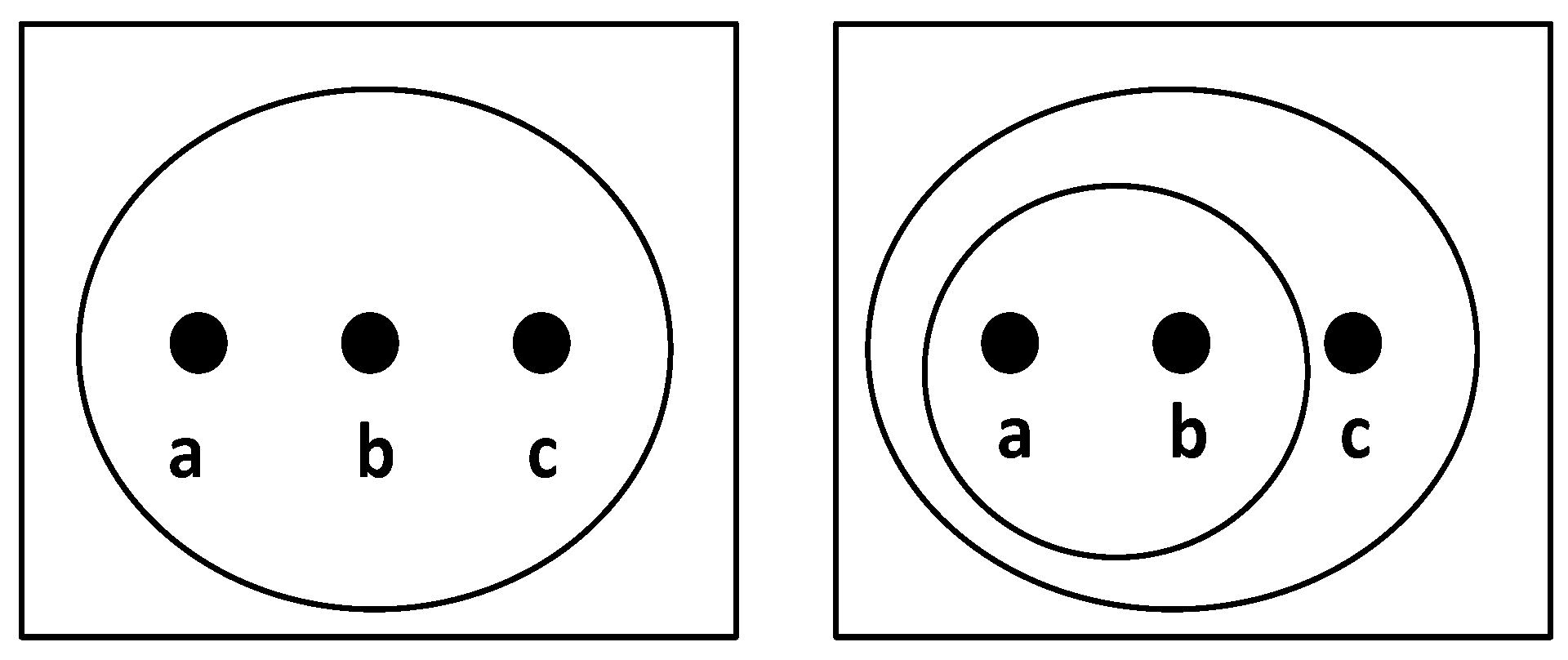
Set X contains three elements, X= {}. Many possible topologies of X can be found. For example, one topology contains X, and another topology contains X, { {},c} as shown in Figure 1.
Points, as well as a set of neighbor points for each point, construct a topological space [11]. Any two topological spaces and have homeomorphism between them, if there is a function f that is continuous, one to one, and a bijection between the two spaces. Then, the two topological spaces would have the same topological type and are basically the same in terms of topology. A widely-known example of homeomorphism is between a donut and a mug. Homology measures connectivity by counting the number of wholes, connected components, faces, and triangles [25]. It can relate a serial of algebraic objects to topological space. A simplex is a topological space made of points, lines, segments, triangles, or their n- dimensional counterparts. A simplical complex consists of multiple simplexes and/or complexes as shown in Figure 2.
2.2. Topological Data Analysis
Topological data analysis is a set of techniques invented to extract insight from data by studying its shape, which is driven from the fact that data has a shape, and a shape has meaning [26]. Topological data analysis is based on algebraic topology, a subfield of topology that aims to quantify shapes using persistent homology. Persistent homology is used to compute the topological features of data at different resolutions by considering different radii from the data points [27]. It increases the radius to connect more data points. The persistent homology concept provides stability and robustness against noise due to the fact that noise cannot be persistent [28]. Topological data analysis studies shapes that have three main properties [29]:
- The shapes are not dependent on specific coordinates,
- the shapes are not changed under any transformation without tearing the shape apart, and
- the shapes are produced in a compressed representation that contains infinite distances.
In topological data analysis, high dimensional data in a point cloud is represented by distances, which are one-dimensional information. Therefore, it is independent of the dimensions of the data as shown in the following example. This makes topological data analysis a powerful technique to address high dimensional data.
Example 2.
On Twitter, let us have two users called and . Each user uses a profile image to represent his/her visual identity. For each user, one vector is used to store the pixels for the user’s profile image, which has 1000 dimensions. For users and , we store their images in vectors A and B, respectively. Cosine similarity is one metric to evaluate the distance or closeness. The cosine similarity between A and B based on their profile images provides the distance or closeness of the two users, which is one-dimensional information.
In order to perform topological data analysis, a mapper algorithm is adapted [8,12,30]. Mapper is a method for topological data analysis. The aim of this algorithm is to extract, simplify and visualize high dimensional data. The mapper algorithm takes an inter-point distance matrix (D ∈, where the number of data points) as the input. As for the parameters, users specify f, called a filter function in mapper, (which is computed for each data point and used to partition the data, such as density estimation), clustering algorithm (such as hierarchical clustering), and a cover method that is responsible for dividing the filter function output ranges of data points into intervals by specifying the number of intervals S, and overlap ratio p. Here, overlap is needed to determine connectivity between two intervals in topological data analysis. All data points in one cluster are in the same interval. All data points in one interval, however, are not necessarily in the same cluster.
Mapper generates a simplicial complex that represents clusters of data points and the relationship between them. The simplicial complex consists of nodes and edges. Each cluster is represented by a node, while edges represent the connectivity between the clusters (if ). Clustering algorithms are used to move from a topological version to a statistical one, where mapper is not dependent on a specific clustering algorithm. A summary of mapper is presented below; for an in-depth description, refer to [12].
Let U = be a finite covering of the space X, so that set A is finite. We define the simplicial complex whose vertex set is the indexing set A, and where a family spans a k-simplex in if and only if corresponding clusters have a point in common. It is necessary to generate reference maps , where X is a given point cloud and Z is the reference metric space. With the reference maps, subsets are constructed. Different filters can be used: density estimation, eccentricity, and graph laplacians [12].
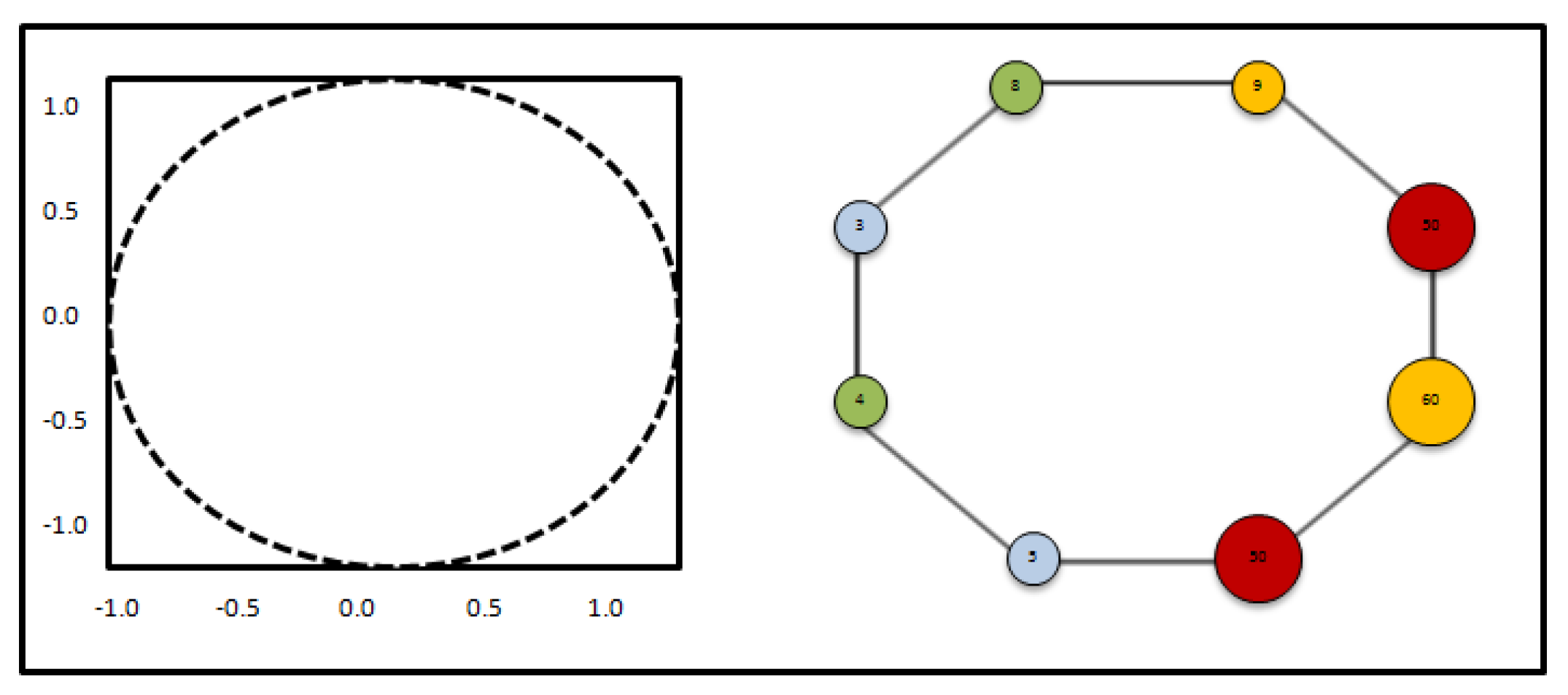
A simple example of a circle using mapper is shown in Figure 3. The left figure is a point cloud of a circle with random variation, X, and the right figure is the simplicial complex of the point cloud, . We arbitrarily selected four levels for this example. The colors represent how filtered the data are. In this example, density estimator is used to filter the data (red being the most dense and blue being the least dense). Edges show the connectivity of clusters of the point cloud. If this is an example of the image popularity analysis, then the left figure is a point cloud of the social media image dataset, and the right is the clustering output of the image dataset from mapper. In addition, the output of mapper can be interpreted in such a way that the shape of the point cloud is a circle, and closer clusters may have higher similarity.
3. Social Network Analysis
Due to the huge amount of data generated from social networks, many researchers investigated several research problems, such as predicting image popularity [16,17,18,19,20,21,22], identifying influential users [31,32], characterizing user behavior [33,34,35,36,37], and detecting community evolution [38,39]. In this paper, the problem of image popularity is addressed.
3.1. Related Work for Image Popularity Prediction
In order to predict image popularity on social networks, researchers have trained several predictive models using many features, including image content, temporal information, and social context [16,17,18,19,20,21,22,23,40].
McParlane et al. [18] predicted the popularity of images on Flickr using an image’s orientation and size, number of faces in an image, most dominant color and the image’s scenes; they classified the images according to a number of scenes based on the image content. They measured popularity using the number of comments and views. Khosla et al. [23] predicted the number of views that images receive on Flickr using images’ colors, gists, textures, and gradients. Can et al. [19] predicted the popularity of images posted on Twitter and Flickr using hash tags, users’ ages, and color histogram; they measured the popularity of images on Twitter using the number of favorites and retweets, and number of views and comments on Flickr. Yamaguchi et al. [41] employed users’ identities, number of posts, number of followers, tags, and images’ colors to predict the popularity of images on Chictopia (a fashion-based social network); they measured popularity based on the number of votes. Totti et al. [42] predicted the popularity of images using aesthetics and users’ information on Pinterest; they measured popularity using the number of repins. Niu et al. [43] predicted the popularity of images on Flickr using network-based features, such as centrality analysis; the number of views was used as a popularity measurement. Gelli [44] used visual sentiments, and users’ information to predict the normalized number of views of images on Flickr. Aloufi et al. [40] used users’ information, number of groups that users belong to, number of tags, images’ colors, gists, and sentiments to predict the popularity of images on Flickr.
Previous works have not addressed noise when building their predictive models. In addition, most studies have only considered low dimensional data. They have focused on the prediction accuracy. Therefore, in this paper, we address the arising issues from the nature of social network data (i.e., high dimensional and noisy data) as well as prediction accuracy.
3.2. Popularity Threshold
As mentioned earlier in this paper, the number of likes is selected as a popularity measurement. However, popularity is subjective. Therefore, we classify the number of likes into popular or unpopular using the Pareto principle as employed in [16,17,18].The Pareto principle () is used in many fields of study, such as business. It is defined as an event where 20% of the causes produce more than 80% of the effects. For example, many companies found out that 80% of their incomes come from 20% of their customers. In our dataset, we observed that 20% of the images receive 99% of the total number of likes, which shows that only 20% of the images attract almost all of the interactions. Using the Pareto principle, a popularity threshold is defined to classify images as popular or unpopular.
3.3. Problems Statement
In this paper, the research problem is formalized differently to fit the topological data analysis approach. We consider it as a clustering problem, where a set of images are clustered together based on a set of features. The percentage of popularity is computed in each cluster, to compute the possibility of popularity in each cluster. Then, the popularity of images is predicted based on the closeness to clusters’ centroids. The approach will be discussed in the following sections. The problem is formalized as follows:
Given a set of images , where each image is represented using a set of features ∀ , and the popularity of images is classified to {1 | 0}, where 0 is for unpopular images, and 1 for popular images. Using the number of likes based on the popularity threshold, a set of images are clustered using the features . The ratio of popularity in each cluster is computed to determine clusters with high or low ratio of popularity. Then, in order to predict the popularity of images, the image will be classified to the cluster that has a centroid with the closest distance to the image.
3.4. Features
In the past, many research papers have shown that image popularity is highly correlated with users’ information, i.e., number of followers of users who uploaded the images [18,19,22,41,42,44], while other research papers showed that popularity can also be related to the content of images [16,17,23,44].
Therefore, we investigate the effects of users’ information and image content on image popularity. In order to represent the users information, the normalized number of followers of users who uploaded the images is selected, while captions are used to represent the images’ contents.
3.4.1. Image Content
Oglesbee [45] states that “Looking at a picture without a caption is like watching television with the sound turned off”. Understanding the meaning of an image can be challenging because the image’s semantic is subjective. Therefore, photographers can describe images using captions, which can provide meanings to images. A caption is a description of an image that accompanies the image. In this paper, we extract the semantics of images using their captions.
In order to extract semantics from captions, a natural language processing technique, Word2vec [46], is used. Word2vec [46] aims to map words that have similar meaning to nearby points using a continuous vector space. When enough data, usage and contexts are provided, Word2vec can guess a word’s meaning based on past appearances using neural network, which is used to learn distributed representations of words; it represents each word in the vector-space using a 300-dimensional vector [46]. These vectors can be used to establish a word’s association with other words in terms of the similarity between the words’ meanings. For example, apple is to fruit is like orange is to fruit.
In our approach, we first tokenized the image’s caption. Then, we remove stopwords and special characters, such as with. Since one caption from each image can have a number of words and each word has its own contribution to the image, all words-vectors from a caption are averaged to make one representative caption vector considering all the contributions of the words for one image. After this, each image has one caption vector with 300 dimensions, , which is computed as follows:
where n represents the number of words, and V represents the 300-dimensional vector for each word.
For example, let us have an image with a caption of “kitchen with refrigerator and oven”. First, we tokenized the words from the caption, we will have five words: [kitchen, with, refrigerator, and, oven]. Then, the stop words are removed. Therefore, [with, and] are removed. The three remaining words will be converted to numerical forms using Word2vec. Each word is represented by a 300-dimensional vector, called v. Finally, we compute the average of the three vectors to represent the image content, . This example is illustrated in Figure 4.
3.4.2. Social Context
As mentioned before, a number of research papers found that the popularity of the user who uploads an image is correlated with the image’s popularity [18,19,22,41,42,44]. In order to represent the users popularity, the normalized number of followers is selected. We normalize the number of followers because we want to focus more on the order of magnitude of the followers, which shows that the ratios among the number of followers are more important than the exact number of followers. The normalized number of followers, i.e., S, is computed as follows:
where ∈ and is the number of followers for user i, while is the maximum number of followers in the dataset.
4. Approach
4.1. Clustering
Topological data analysis can be generalized to solve various problems. As mentioned earlier, the input to mapper is a distance matrix, while the output is a set of clusters.
A distance matrix is a square matrix that represents the distances between the elements in a set [47]. Since there are many problems that can be solved using clustering algorithms, topological data analysis can be adapted. Moreover, any distance metric can be used, such as Euclidean or cosine similarity.
For the content feature, we compute the distances between any two images i and j using the cosine similarity [48], called , of their 300-dimensional caption vectors, i.e., , which is calculated as follows:
Cosine similarity is used because the similarity between and is shown using the directions of the two vectors. For the social context feature, we compute the distances between any two images i and j using the Euclidean distance [49] of their one-dimensional feature, called D, which is calculated as follows:
Euclidean distance is used because the distance between any two users based on their number of followers is shown by computing the difference between the number of followers each user has.
With these distances, a distance matrix M is created for each feature. Then, each distance matrix is employed separately to mapper to cluster the data to analyze the relationship between the popularity of images and each feature.
Because the rule was used to determine popularity, the ratio of popular images in each cluster is normalized by . Therefore, if the normalized ratio of popular images in a cluster is , then the effects of the feature on the popularity of the cluster were neutral. However, if the ratio of popularity is greater than , the popularity ratio is considered high, while if the ratio is less than , it is considered as a low ratio of popularity.
Regarding the images’ popularity, the clusters can be classified into three groups: low possibility of popularity, ; neutral, ; and high possibility of popularity, , based on the criteria discussed above. If an image falls into , then it can be said that the image has a higher possibility of becoming popular, and if an image falls into , it has a lower possibility of becoming popular. Note that the ratio of popularity in each clusters is computed for three intervals: during first hour, after first day, and after the first week. Therefore, an image can belong to in the first hour, then belongs to after the first day, if the ratio of the popularity in that cluster increases after one day.
4.2. Prediction
Our mechanism predicts image popularity based on the cluster with the nearest centroid, which is determined by computing the distance between each image and the cluster’s centroid. The centroid of a cluster d, i.e., is computed as follows:
where N represents the number of images in the cluster d, while x contains the images in the cluster, which are represented using either of the two features discussed earlier.
For the prediction of images using the image content’s feature, the cosine similarity distance is used to compute the distance. Therefore, in order to predict the popularity of images, the nearest cluster’s centroid is determined by finding the cluster with the centroid that has the highest cosine similarity with the image’s content. The objective function is computed as follows:
where y represents the cluster with the highest cosine similarity to the image’s content.
On the other hand, for predicting the popularity of images using the social context’s feature, Euclidean distance is used. In this case, the images will belong to the cluster that has the shortest distance to the image’s social context. In this case, the objective function will change slightly, which is computed as follows:
where y represents the cluster with the shortest Euclidean distance to the image’s social context.
Moreover, the images in our dataset are already labeled into popular and unpopular images using the Pareto principle as discussed in Section 3.2; therefore, we use these labels to determine whether the images are assigned to the correct clusters, i.e., or or not. For example, if an image is popular, and clustered to one of the clusters, it means that it is correctly identified as popular. If an image is clustered in one of the clusters, and the image is unpopular, it means that it is correctly identified as unpopular. However, if a popular image is clustered to , this means that it is not correctly identified as a popular image. In our experiments, we predict both the popular and unpopular images.
5. Experimental Setup
5.1. Instagram Dataset
We crawled our dataset from Instagram using given users IDs; based on our experiment with the Instagram API, we observed that users’ IDs are simply numbered from one to millions. Therefore, we randomly selected more than 1,000,000 IDs. Using these IDs, we triggered the Instagram API to retrieve users. We found 149,520 users with public security settings. However, among these users, there are 89,093 who shared at least ten images. We use these users because they are active. We retrieved 69,000 images that were uploaded during the first hour when we triggered the API. However, after preprocessing, we had 49,045 images. Then, the same images are checked again after one day and after one week to track the changes in the number of likes. After applying the rule, the popularity thresholds of the data set for one hour, one day and one week are measured. The data has been randomly split into training and testing datasets: for training and for testing. The training dataset contains 32,920 images, while the testing dataset contains 14,108 images.
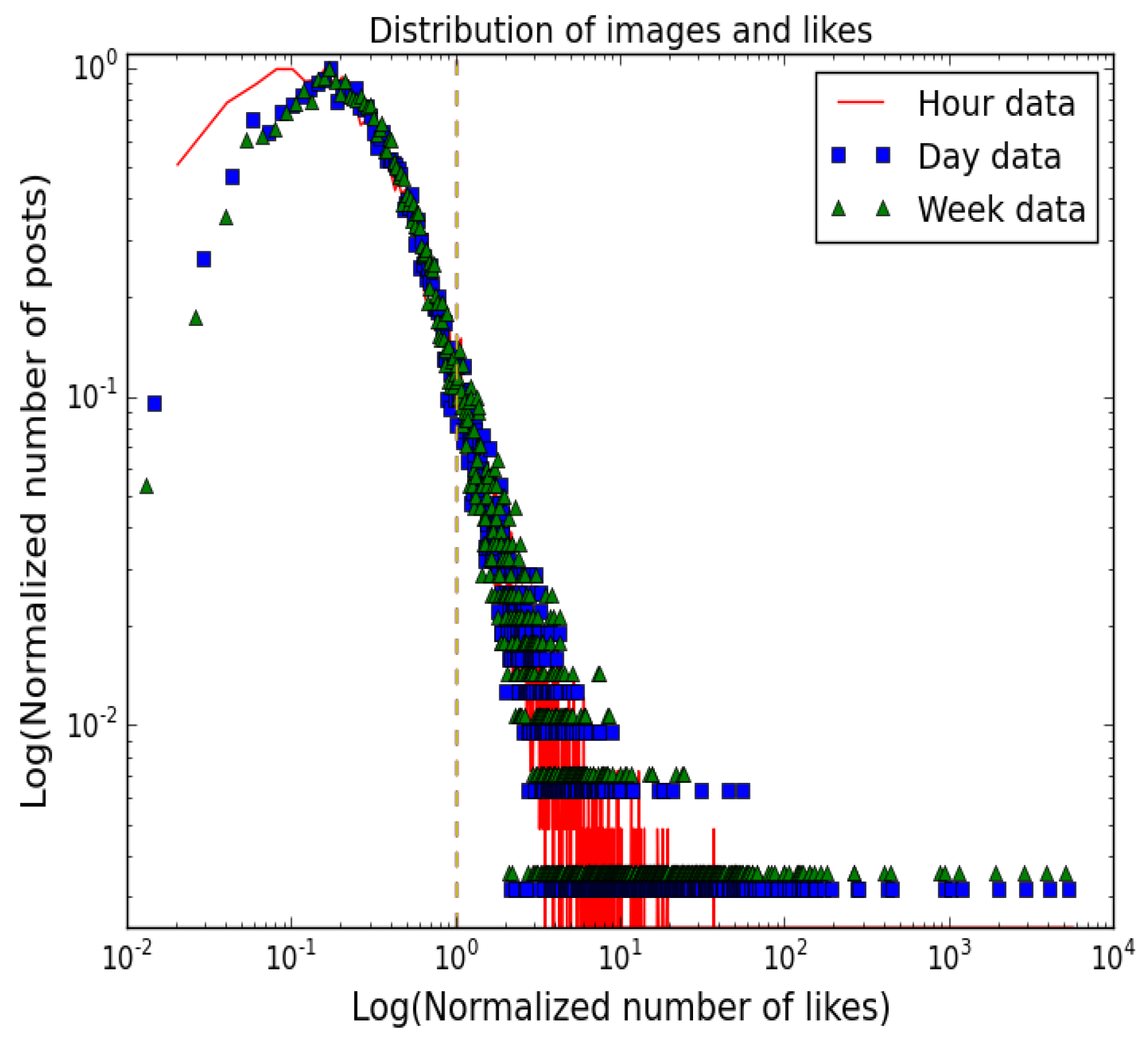
Table 1 shows the popularity thresholds for different time frames after applying the Pareto principle on the number of likes. The popularity thresholds are: 45 during the first hour, 69 after the first day, and 75 after the first week. Any image that receives a number of likes that is greater or equal to these thresholds is considered popular during these time frames. For example, if an image received 50 likes in one hour, 70 likes after one day and 71 likes after one week, it implies that this image was popular during the first hour and after the first day, but became unpopular after one week.
Figure 5 shows the plots of the number of images with respect to the number of likes in the one hour data, one day data and one week data. Both axes are log scaled. The y-axis represent the number of images; it is normalized by the maximum number of images, so the peak points at one. The x-axis represents the normalized number of likes. They are normalized by the popularity threshold from Table 1, so the threshold lines overlap each other and form one vertical dotted line. The normalized distributions shown in Figure 5 are similar to each other, and the popularity thresholds are also synchronized within the distributions. The figure shows that the distribution of images and likes over different time frames exhibits similar trends relatively; this can mean that there is a possibility that early information about popularity can be used to predict future popularity. It also indicates that the popularity of images are saturated in within the first hour of image upload. In addition, one note on the one hour set is that the peak in the low number of likes partly shows a deviation from the others. It may be from being in the process of maturity.
5.2. Implementation
As mentioned earlier, a mapper [30] is implemented to perform topological data analysis. It is available through a Python package. We have used Density estimation as the filter function.
In order to convert captions to numerical form, Gensim, a Python library that implements Word2vec (https://code.google.com/archive/p/word2vec/) is used [50]. The Word2vec model is trained using 100 billion words from Google News and achieves an accuracy rate of 73%.
In order to compare topological data analysis and clustering algorithms, k-means and hierarchical clustering are implemented. Hierarchical clustering is implemented using Scikit-learn [51]; we have used an average linkage, and for connectivity, we have employed kneighbors graph algorithm. In order to determine the cut-off, we have used the parameter in [51].
In addition, k-means is implemented using the Natural Language ToolKit [52]. For selecting the initial means, k-means++ is used [53]. Both packages are implemented in Python. The number of clusters varies between 5 and 15 to observe their effects on popularity; however, only experiments with five clusters are presented since the results are almost identical.
5.3. Evaluation
In order to evaluate the accuracy of the three approaches, the F-score is computed. F-score computes both precision and recall to compute the accuracy of the test, which represents the harmonic mean of precision and recall. It is computed as below:
We compute the F-score for both prediction classes: popular and unpopular images.
6. Empirical Results Using Topological Data Analysis
In this section, we discuss the experiments and results for topological data analysis. We employ topological data analysis using the two features discussed earlier to cluster the images in the training dataset and then compute the ratio of popularity in each cluster to identify clusters with high or low ratios of popularity. The number of intervals used in the experiment is five as mentioned earlier. Then, we predict the popularity of images using the proposed approach.
6.1. Clustering
First, we employed the mapper using the image content feature. The results show that from cluster 1 to cluster 5, the ratios of popular images increases. Cluster 1 has the lowest ratio, lower than neutral, and cluster 5 has the highest, higher than neutral, while clusters 2–4 have neutral ratios of popularity. Therefore, we assigned cluster 1 to , cluster 2–4 to and cluster 5 to .
Next, we employed the social context feature to the mapper, and the results show that the ratios of popularity have increased significantly. In this experiment, the ratios of popularity decreased from clusters one to five, which produces a monotonic decrease relationship between the clusters. Cluster 1 has the highest ratio of popularity, higher than neutral, while cluster 5 has the lowest ratio of popularity, lower than neutral. No cluster with a neutral ratio of popularity is observed in this experiment. Clusters 1 and 2 are assigned to , while the remaining clusters are assigned to .
6.2. Prediction
In this experiment, we have predicted the popular and unpopular images using the two features. Using the image content, topological data analysis achieved an accuracy of for predicting the popular images during the first hour. The accuracy of prediction have stayed the same for first day and first week periods. As for the prediction of unpopular images, topological data analysis achieved an accuracy of for the first hour prediction. Then, the accuracy has decreased to for the first day and first week periods.
On the other hand, the results have increased significantly when the social context is used. During the first hour, topological data analysis achieves an accuracy of for predicting the popular images. For predicting the unpopular images, the accuracy has increased to . For both prediction of popular and unpopular images, the accuracy stayed the same over the first day and week periods. The results are summarized in Table 2. For both features, the accuracy rates for the prediction of unpopular images are higher than the accuracy rates for the prediction of popular images because of the images in our dataset are unpopular based on the Pareto principle.
7. Empirical Results Using Clustering Algorithms
In order to compare the topological data analysis approach with the clustering algorithms, we employed k-means and hierarchical clustering. In addition, the same distance metrics that are used for topological data analysis are used for k-means and hierarchical clustering.
7.1. k-Means
K-means [54] is one of the most popular clustering algorithms. It clusters data into a set of clusters, i.e., k, based on the nearest mean. In k-means, connectivity has no meaning. Therefore, there are no relationships between clusters. K-means is employed using both features.
7.1.1. Clustering
First, we employed the image content feature, and the results show that clusters 2–5 have neutral ratios of popularity and are assigned to . However, cluster 1 has a low ratio of popularity, lower than neutral, and therefore is assigned to .
Second, the social context feature is used. The ratios of popularity have increased significantly as observed using topological data analysis. The result shows that clusters 2 and 3 have low ratios of popularity, lower than neutral and lower than neutral, respectively. They are assigned to . Other clusters have high ratios of popularity. Cluster 4 has a perfect ratio of popularity, at 100%. Cluster 5 has a popularity ratio that is 58% higher than neutral, while cluster 1 has a ratio that is 232% higher than neutral. Clusters 1 and 4–5 are assigned to .
7.1.2. Prediction
As discussed in the previous subsection, k-means failed to find any cluster with a high ratio of popularity when the image content is employed. Therefore, the prediction accuracy rate for predicting the popular images is . However, for predicting the unpopular images, k-means achieved an accuracy rate of for the first hour prediction, and then the accuracy rate has decreased to for the first day and week.
On the other hand, the accuracy rate of popular images using the social context have increased significantly to . Moreover, the accuracy rates for predicting the unpopular images have increased to . For the two predictions, the accuracy rates have stayed the same over the three time frames. The results are summarized in Table 3.
7.2. Hierarchical Clustering
In hierarchical clustering algorithm [55], clustering is performed differently than k-means. It builds a hierarchy of clusters. In hierarchical clustering, connectivity exists. Therefore, relationships exist between clusters.
7.2.1. Clustering
Using the image content feature, the result shows a new case, which occurred in cluster 4. Cluster 4 has a popularity ratio = 0, which means that in this cluster, the possibility for an image to become popular is . This cluster is assigned to . The remaining clusters have neutral ratios of popularity and are assigned to . However, the ratio of popularity in cluster 1 has become higher than neutral after the first hour. Therefore, cluster 1 is assigned to for the first day and week periods. For the connectivity part, no meaningful trend is detected.
Next, we employed the social context feature, and as observed in the other experiments that are based on the social context feature, the ratios of popularity have increased significantly. Cluster 4 has a popularity ratio of 0. Cluster 1 has a ratio that is lower than neutral. Both clusters are assigned to . Clusters 3, 4 and 5 have high ratios of popularity: , , and higher than neutral, respectively. They are assigned to . Moreover, the connectivity between these clusters is represented as a monotonic increase in the ratios of popularity along the connected clusters.
7.2.2. Prediction
As discussed in the previous subsection, hierarchical clustering failed to find any clusters with a high ratio of popularity during the first hour using the image content feature. Therefore, the accuracy rate for predicting the popular images is during the first hour. However, as mentioned earlier, the ratio of popularity in cluster 1 has become higher than neutral; therefore, hierarchical clustering predicted popular images with an accuracy rate of for the first day and week time frames. For predicting the unpopular images, hierarchical clustering achieved an accuracy of 49% during the first hour, and 18% for the first day and week.
As for the social context feature, the accuracy rate for predicting the popular images has increased significantly to . Moreover, the accuracy rates for predicting the unpopular images have increased to . For the two predictions, the accuracy rates have stayed the same over the thee time periods. The results are summarized in Table 4.
8. Comparison
In this section, we will compare between the performance of the three approaches in terms of accuracy using the two features.
8.1. Image Content
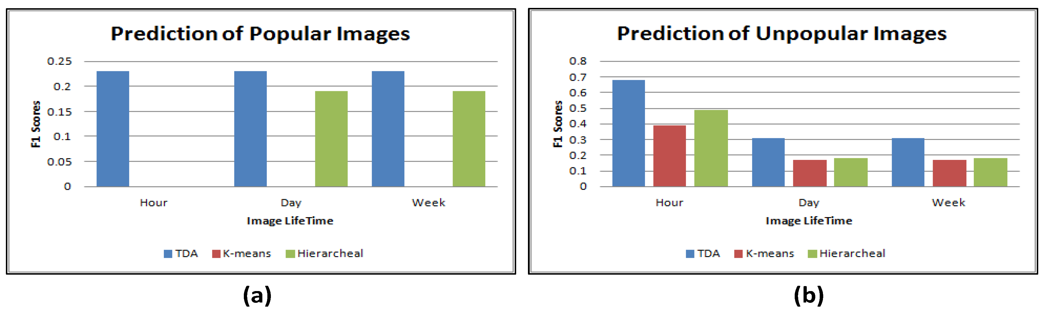
Figure 6 plots the accuracy rates for predicting the popular and unpopular images using the three approaches. The results show that topological data analysis outperforms the other approaches for predicting the popular and unpopular images. This shows that topological data analysis performs better than traditional data mining techniques when a high dimensional feature is employed, i.e., image content. In terms of the changes in the prediction accuracy rates over time, three approaches achieved high accuracy rates for predicting the unpopular images during the first hour. However, the accuracy rates decreased after that. However, for predicting the popular images, the three approaches have the same accuracy rated over different time frames, except for hierarchical clustering, because, as discussed before, during the first hour, hierarchical clustering could not find any cluster with a high ratio of popular images. The results show that the popularity of images is saturated during the first week.
8.2. Social Context
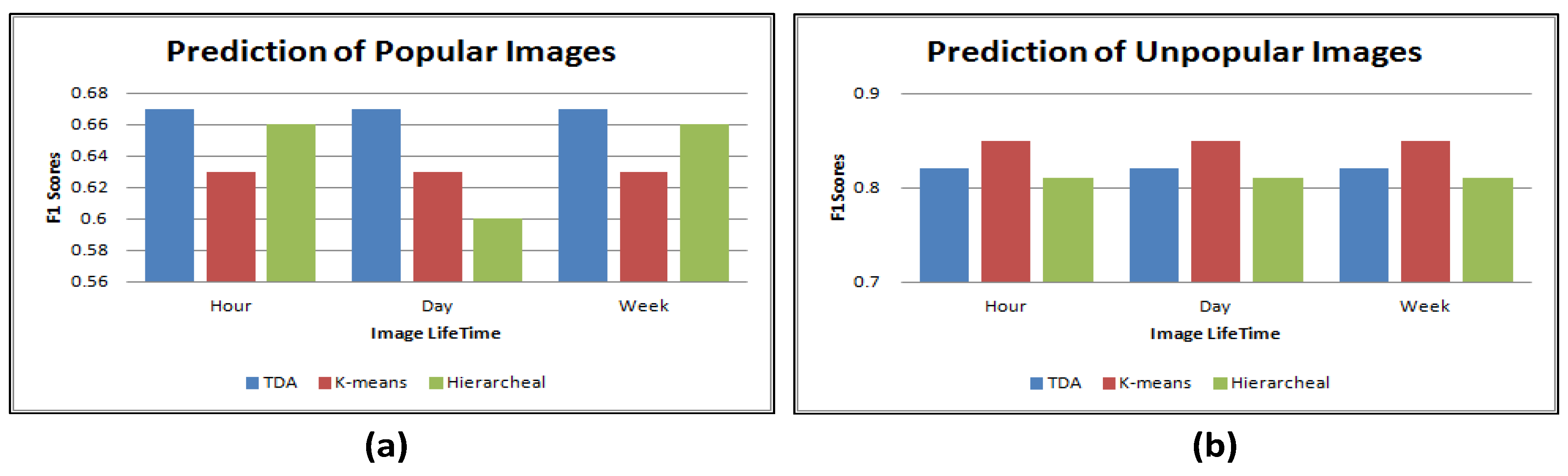
The three approaches have very similar accuracy rates for predicting the popular and unpopular images. For predicting the popular images, topological data analysis slightly improves the accuracy rate with 1% more than hierarchical clustering and 4% more than k-means. As for predicting the unpopular images, k-means slightly improves the accuracy with 3% higher than topological data analysis, and 4% higher than hierarchical clustering. In terms of changes of accuracy rates over time, no changes are observed. The results show that when using a low dimensional feature, i.e., social context, traditional data mining techniques perform as well as topological data analysis.
9. Discussion
In this paper, the feasibility of topological data analysis for mining social network data is explored. We addressed the problem of image popularity by analyzing the effects of image content and social context on image popularity. In order to address this problem, we randomly crawled images along with their metadata from Instagram. We first converted the images’ captions to numerical vectors using Word2vec. In addition, the normalized number of followers is used to represent the social context. Then, we calculated the distances of each feature and applied it to mapper. These features are then employed to k-means and hierarchical clustering for comparing topological data analysis and clustering algorithms. Then, we predicted both the popular and unpopular images based on how close the images are to the centroid of the clusters. The results exhibited several outcomes:
- Topological data analysis is feasible for social network analysis and mining;
- Image content and social context have correlations to image popularity;
- Topological data analysis significantly outperformed traditional clustering algorithms using the high dimensional feature, i.e., image content. It achieved higher accuracy rates than k-means and hierarchical clustering algorithms. It also generated a meaningful connectivity between the clusters, i.e., a monotonic increase in the popularity ratio along the connected clusters;
- For predicting the popularity of images using the low dimensional feature, i.e., social context, traditional data mining techniques perform as well as topological data analysis;
- The results show that using the context feature improves the accuracy rates significantly, which confirms that the popularity of images is highly related to users’ popularity;
- For the changes of popularity over time, a trend is only observed for the prediction of popular images using the image content;
- Lastly, the results show that popularity of images is saturated in a short period of time.
10. Conclusions
In conclusion, in order to address high dimensional and noisy data, topological data analysis proved to outperform traditional clustering algorithms. It also showed that the geometric shape of data matters and can be adopted to produce meaningful information. With regard to future work, it would be interesting to investigate feature integration using topological data analysis since topological data analysis relies on distances.
Acknowledgments
The authors acknowledge the University of Bridgeport for providing the necessary resources to carry this research conducted in the Multimedia Information Group under the supervision of Jeongkyu Lee. The cost of publishing this paper was funded by the University of Bridgeport, CT, USA.
Author Contributions
This research is part of Khaled Almgren Ph.D. dissertation work under the supervision of Jeongkyu Lee. Extensive discussions about the algorithms and techniques presented in this paper were carried between the authors; Minkyu Kim advised Khaled Almgren in designing and conceiving the experiments; Khaled Almgren performed the exmperiments; Manuscript was written by Khaled Almgren; All authors reviewed and approved the final manuscript.
Conflicts of Interest
The authors declare no conflict of interest.
References
- Twitter. Twitter Usage. 2016. Available online: https://about.twitter.com/company (accessed on 13 April 2017).
- Facebook. Facebook Stats. 2016. Available online: https://newsroom.fb.com/company-info/ (accessed on 13 April 2017).
- Instagram. Instagram Stats. 2016. Available online: https://business.instagram.com (accessed on 13 April 2017).
- Wu, X.; Zhu, X.; Wu, G.Q.; Ding, W. Data mining with big data. IEEE Trans. Knowl. Data Eng. 2014, 26, 97–107. [Google Scholar]
- Fan, J.; Han, F.; Liu, H. Challenges of big data analysis. Natl. Sci. Rev. 2014, 1, 293–314. [Google Scholar] [CrossRef] [PubMed]
- Becker, H.; Naaman, M.; Gravano, L. Event Identification in Social Media. In Proceedings of the International Workshop on the Web and Databases, Snowbird, UT, USA, 22 June 2014. [Google Scholar]
- Edelsbrunner, H.; Letscher, D.; Zomorodian, A. Topological persistence and simplification. In Proceedings of the 41st Annual Symposium on Foundations of Computer Science, Washington, DC, USA, 12–14 November 2000; pp. 454–463. [Google Scholar]
- Carlsson, G. Topology and data. Bull. Am. Math. Soc. 2009, 46, 255–308. [Google Scholar] [CrossRef]
- Nicolau, M.; Tibshirani, R.; Børresen-Dale, A.L.; Jeffrey, S.S. Disease-specific genomic analysis: Identifying the signature of pathologic biology. Bioinformatics 2007, 23, 957–965. [Google Scholar] [CrossRef] [PubMed]
- Nicolau, M.; Levine, A.J.; Carlsson, G. Topology based data analysis identifies a subgroup of breast cancers with a unique mutational profile and excellent survival. Proc. Natl. Acad. Sci. USA 2011, 108, 7265–7270. [Google Scholar] [CrossRef] [PubMed]
- Choudhary, D.; Bansal, S. Topological Data Analysis. 2014. Available online: https://cse.iitk.ac.in/users/cs365/2014/submissions/deepakc/project/report.pdf (accessed on 14 July 2017).
- Singh, G.; Mémoli, F.; Carlsson, G.E. Topological methods for the analysis of high dimensional data sets and 3D object recognition. In Proceedings of the 2007 Symposium on Point-Based Graphics, Prague, Czech Republic, 2–3 September 2007; pp. 91–100. [Google Scholar]
- Gidea, M.; Katz, Y.A. Topological Data Analysis of Financial Time Series: Landscapes of Crashes. arXiv, 2017; arXiv:1703.04385. [Google Scholar] [CrossRef]
- Schebesch, K.B.; Stecking, R.W. Topological Data. In Operations Research Proceedings 2015; Springer: Cham, Switzerland, 2017; pp. 483–489. [Google Scholar]
- Webster, M. The Merriam-Webster Dictionary; Merriam-Webster: Springfield, MA, USA, 2005. [Google Scholar]
- Almgren, K.; Lee, J.; Kim, M. Predicting the Future Popularity of Images on Social Networks. In Proceedings of the 3rd Multidisciplinary International Social Networks Conference on SocialInformatics, Union, NJ, USA, 15–17 August 2016; p. 15. [Google Scholar]
- Almgren, K.; Lee, J.; Kim, M. Prediction of image popularity over time on social media networks. In Proceedings of the IEEE Annual Connecticut Conference on Industrial Electronics, Technology & Automation (CT-IETA), Bridgeport, CT, USA, 14–15 October 2016; pp. 1–6. [Google Scholar]
- McParlane, P.J.; Moshfeghi, Y.; Jose, J.M. Nobody comes here anymore, it’s too crowded; predicting image popularity on flickr. In Proceedings of the International Conference on Multimedia Retrieval, Glasgow, UK, 1–4 April 2014; p. 385. [Google Scholar]
- Can, E.F.; Oktay, H.; Manmatha, R. Predicting retweet count using visual cues. In Proceedings of the 22nd ACM International Conference on Information & Knowledge Management, San Francisco, CA, USA, 27 October–1 November 2013; pp. 1481–1484. [Google Scholar]
- Guille, A.; Hacid, H.; Favre, C.; Zighed, D.A. Information diffusion in online social networks: A survey. ACM SIGMOD Rec. 2013, 42, 17–28. [Google Scholar] [CrossRef]
- Bakshy, E.; Rosenn, I.; Marlow, C.; Adamic, L. The role of social networks in information diffusion. In Proceedings of the 21st International Conference on World Wide Web, Lyon, France, 16–20 April 2012; pp. 519–528. [Google Scholar]
- Cappallo, S.; Mensink, T.; Snoek, C.G. Latent factors of visual popularity prediction. In Proceedings of the 5th ACM on International Conference on Multimedia Retrieval, Shanghai, China, 23–26 June 2015; pp. 195–202. [Google Scholar]
- Khosla, A.; Das Sarma, A.; Hamid, R. What makes an image popular? In Proceedings of the 23rd International Conference on World Wide Web; pp. 867–876.
- Munkres, J.R. Topology; Prentice Hall: Upper Saddle River, NJ, USA, 2000. [Google Scholar]
- Cartan, H.; Eilenberg, S. Homological Algebra (PMS-19); Princeton University Press: Princeton, NJ, USA, 2016; Volume 19. [Google Scholar]
- Murphy, N. Topological Data Analysis. 2016. Available online: https://www.colby.edu/math/program/honorsprojects/2016-Murphy-HonorsThesis.pdf (accessed on 14 July 2017).
- Zomorodian, A.; Carlsson, G. Computing persistent homology. Discret. Comput. Geom. 2005, 33, 249–274. [Google Scholar] [CrossRef]
- Cohen-Steiner, D.; Edelsbrunner, H.; Harer, J. Stability of persistence diagrams. Discret. Comput. Geom. 2007, 37, 103–120. [Google Scholar] [CrossRef]
- Michel, B. Statistics and Topological Data Analysis. Available online: https://www.turing-gateway.cam.ac.uk/sites/default/files/asset/doc/1606/BertrandMichel.pdf (accessed on 14 July 2017).
- Müllner, D.; Babu, A. Python Mapper: An Open-Source Toolchain for Data Exploration, Analysis and Visualization. 2013. Available online: http://danifold.net/mapper (accessed on 14 July 2017).
- Erlandsson, F.; Bródka, P.; Borg, A.; Johnson, H. Finding influential users in social media using association rule learning. Entropy 2016, 18, 164. [Google Scholar] [CrossRef]
- Almgren, K.; Lee, J. An empirical comparison of influence measurements for social network analysis. Soc. Netw. Anal. Min. 2016, 6, 52. [Google Scholar] [CrossRef]
- Chen, W.; Gao, Q.; Xiong, H. Temporal Predictability of Online Behavior in Foursquare. Entropy 2016, 18, 296. [Google Scholar] [CrossRef]
- Li, Y.; Wu, C.; Luo, P.; Zhang, W. Exploring the characteristics of innovation adoption in social networks: Structure, homophily, and strategy. Entropy 2013, 15, 2662–2678. [Google Scholar] [CrossRef]
- Rodríguez Barraquer, T. From Observable Behaviors to Structures of Interaction in Binary Games of Strategic Complements. Entropy 2013, 15, 4648–4667. [Google Scholar] [CrossRef]
- Silva, T.H.; de Melo, P.O.V.; Almeida, J.M.; Salles, J.; Loureiro, A.A. A picture of Instagram is worth more than a thousand words: Workload characterization and application. In Proceedings of the 2013 IEEE International Conference on Distributed Computing in Sensor Systems (DCOSS), Cambridge, MA, USA, 20–23 May 2013; pp. 123–132. [Google Scholar]
- Mejova, Y.; Haddadi, H.; Noulas, A.; Weber, I. #Foodporn: Obesity patterns in culinary interactions. In Proceedings of the 5th International Conference on Digital Health, Florence, Italy, 18–20 May 2015; pp. 51–58. [Google Scholar]
- Saganowski, S.; Gliwa, B.; Bródka, P.; Zygmunt, A.; Kazienko, P.; Koźlak, J. Predicting community evolution in social networks. Entropy 2015, 17, 3053–3096. [Google Scholar] [CrossRef]
- Xu, H.; Hu, Y.; Wang, Z.; Ma, J.; Xiao, W. Core-based dynamic community detection in mobile social networks. Entropy 2013, 15, 5419–5438. [Google Scholar] [CrossRef]
- Aloufi, S.; Zhu, S.; El Saddik, A. On the Prediction of Flickr Image Popularity by Analyzing Heterogeneous Social Sensory Data. Sensors 2017, 17, 631. [Google Scholar] [CrossRef] [PubMed]
- Yamaguchi, K.; Berg, T.L.; Ortiz, L.E. Chic or social: Visual popularity analysis in online fashion networks. In Proceedings of the 22nd ACM International Conference on Multimedia, Orlando, FL, USA, 3–7 November 2014; pp. 773–776. [Google Scholar]
- Totti, L.C.; Costa, F.A.; Avila, S.; Valle, E.; Meira, W., Jr.; Almeida, V. The impact of visual attributes on online image diffusion. In Proceedings of the 2014 ACM Conference on Web Science, Bloomington, IN, USA, 23–26 June 2014; pp. 42–51. [Google Scholar]
- Niu, X.; Li, L.; Mei, T.; Shen, J.; Xu, K. Predicting image popularity in an incomplete social media community by a weighted bi-partite graph. In Proceedings of the 2012 IEEE International Conference on Multimedia and Expo (ICME), Melbourne, VIC, Australia, 9–13 July 2012; pp. 735–740. [Google Scholar]
- Gelli, F.; Uricchio, T.; Bertini, M.; Del Bimbo, A.; Chang, S.F. Image popularity prediction in social media using sentiment and context features. In Proceedings of the 23rd ACM International Conference on Multimedia, Brisbane, QLD, Australia, 26–30 October 2015; pp. 907–910. [Google Scholar]
- Oglesbee, L. Writing Captions. Commun. J. Educ. Today 1998, 32, 2–6. [Google Scholar]
- Mikolov, T.; Chen, K.; Corrado, G.; Dean, J. Efficient estimation of word representations in vector space. arXiv, 2013; arXiv:1301.3781. [Google Scholar]
- Bonchev, D.; Trinajstić, N. Information theory, distance matrix, and molecular branching. J. Chem. Phys. 1977, 67, 4517–4533. [Google Scholar] [CrossRef]
- Larsen, B.; Aone, C. Fast and effective text mining using linear-time document clustering. In Proceedings of the Fifth ACM SIGKDD International Conference On Knowledge Discovery and Data Mining, San Diego, CA, USA, 15–18 August 1999; pp. 16–22. [Google Scholar]
- Deza, M.M.; Deza, E. Encyclopedia of distances. In Encyclopedia of Distances; Springer: Berlin/Heidelberg, Germany, 2009; pp. 1–583. [Google Scholar]
- Rehurek, R.; Sojka, P. Gensim–Python Framework for Vector Space Modelling; Masaryk University: Brno, Czech Republic, 2011. [Google Scholar]
- Pedregosa, F.; Varoquaux, G.; Gramfort, A.; Michel, V.; Thirion, B.; Grisel, O.; Blondel, M.; Prettenhofer, P.; Weiss, R.; Dubourg, V.; et al. Scikit-learn: Machine learning in Python. J. Mach. Learn. Res. 2011, 12, 2825–2830. [Google Scholar]
- Bird, S. NLTK: The natural language toolkit. In Proceedings of the COLING/ACL on Interactive Presentation Sessions, Sydney, NSW, Australia, 17–18 July 2006; Association for Computational Linguistics: Stroudsburg, PA, USA, 2006; pp. 69–72. [Google Scholar]
- Arthur, D.; Vassilvitskii, S. k-means++: The advantages of careful seeding. In Proceedings of the Eighteenth Annual ACM-SIAM Symposium on Discrete Algorithms, New Orleans, Louisiana, 7–9 January 2007; Society for Industrial and Applied Mathematics: Philadelphia, PA, USA, 2007; pp. 1027–1035. [Google Scholar]
- Hartigan, J.A.; Wong, M.A. Algorithm AS 136: A k-means clustering algorithm. J. R. Stat. Soc. Ser. C 1979, 28, 100–108. [Google Scholar] [CrossRef]
- Johnson, S.C. Hierarchical clustering schemes. Psychometrika 1967, 32, 241–254. [Google Scholar] [CrossRef] [PubMed]
Figure 1.
Possible topologies of set X. In the left diagram, , while is in the right diagram.

Figure 2.
The upper diagrams are examples of simplexes: a point, a line, a triangle, and a tetrahedron. The lower diagrams are examples of a simplicial complex: many triangles with many lines and one triangle with one line.
Figure 2.
The upper diagrams are examples of simplexes: a point, a line, a triangle, and a tetrahedron. The lower diagrams are examples of a simplicial complex: many triangles with many lines and one triangle with one line.
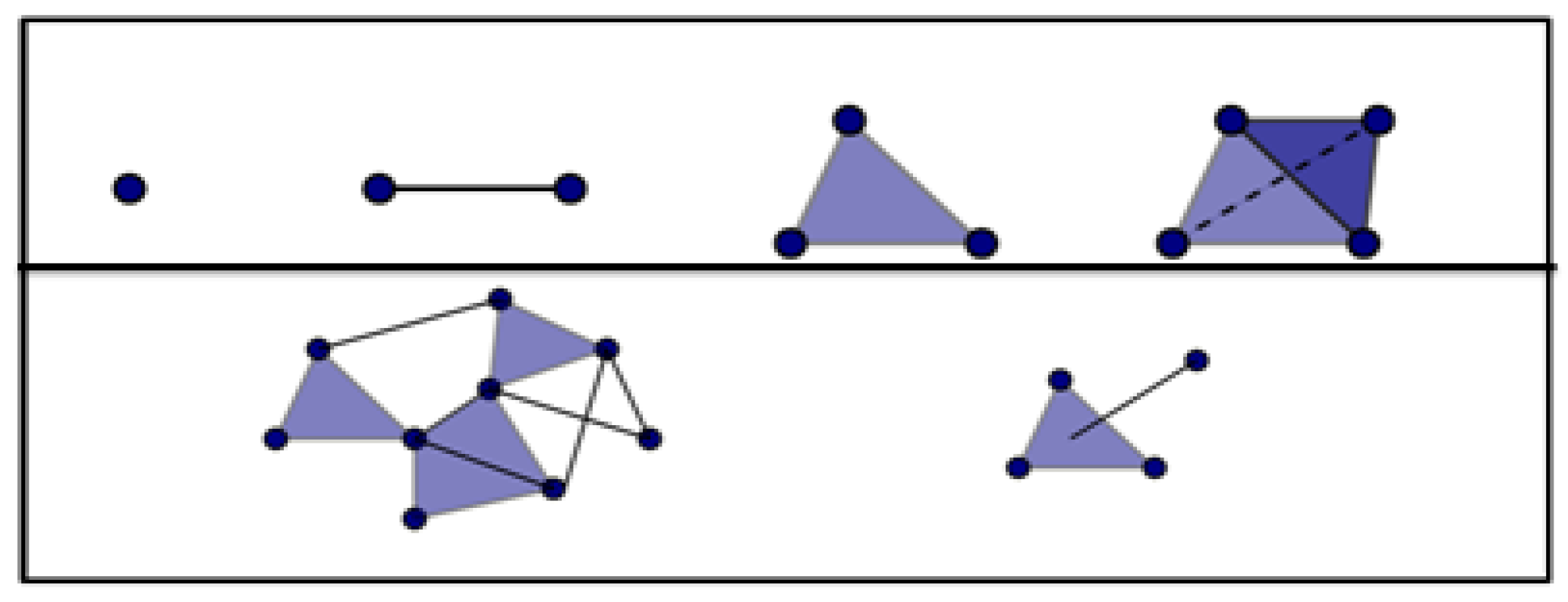
Figure 3.
A unit circle and the result of topological analysis using mapper. The size of the nodes on the right indicate the size of the cluster, and the numbers written inside the nodes indicate the number of data points.
Figure 3.
A unit circle and the result of topological analysis using mapper. The size of the nodes on the right indicate the size of the cluster, and the numbers written inside the nodes indicate the number of data points.

Figure 4.
An example of how the image content is represented.
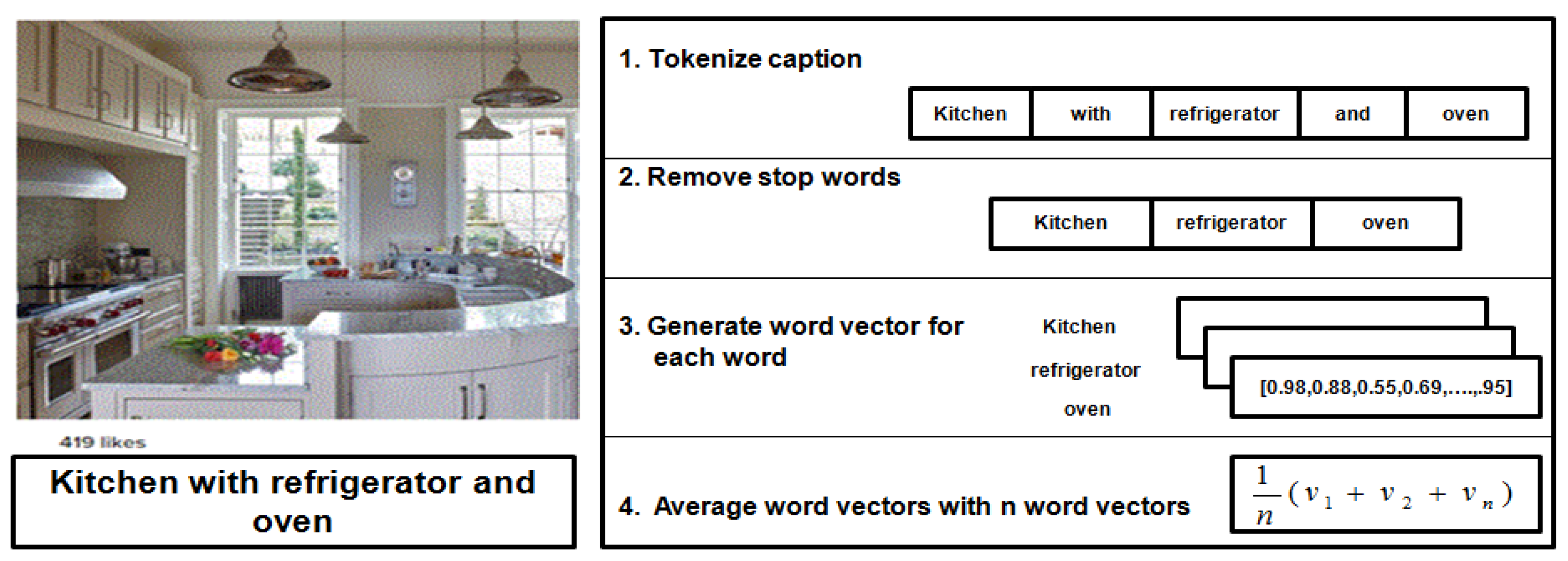
Figure 5.
Distribution of the number of images vs. the number of likes. Both axes are normalized.

Figure 6.
Accuracy rates for the three approaches using for the image content feature. (a) prediction of popular images; (b) prediction of unpopular images.
Figure 6.
Accuracy rates for the three approaches using for the image content feature. (a) prediction of popular images; (b) prediction of unpopular images.

Figure 7.
Accuracy rates for the three approaches using for the social context feature. (a) prediction of popular images; (b) prediction of unpopular images.
Figure 7.
Accuracy rates for the three approaches using for the social context feature. (a) prediction of popular images; (b) prediction of unpopular images.


Table 1.
Popularity thresholds of the number of likes in different time frames.
| Popularity Thresholds | 1 Hour | 1 Day | 1 Week |
|---|---|---|---|
| Number of Likes | 45 | 69 | 75 |
Table 2.
Accuracy of topological data analysis for predicting the popular and unpopular images using the image content and social context.
Table 2.
Accuracy of topological data analysis for predicting the popular and unpopular images using the image content and social context.
| Periods | Accuracy Rates | |||
|---|---|---|---|---|
| Image Content | Social Context | |||
| Popular Images | Unpopular Images | Popular Images | Unpopular Images | |
| Hour | 0.23 | 0.68 | 0.67 | 0.82 |
| Day | 0.23 | 0.31 | 0.67 | 0.82 |
| Week | 0.23 | 0.23 | 0.67 | 0.82 |
Table 3.
Accuracy of k-means for predicting the popular and unpopular images using the image content and social context.
Table 3.
Accuracy of k-means for predicting the popular and unpopular images using the image content and social context.
| Periods | Accuracy Rates | |||
|---|---|---|---|---|
| Image Content | Social Context | |||
| Popular Images | Unpopular Images | Popular Images | Unpopular Images | |
| Hour | 0 | 0.39 | 0.85 | 0.63 |
| Day | 0 | 0.17 | 0.85 | 0.63 |
| Week | 0 | 0.17 | 0.85 | 0.63 |
Table 4.
Accuracy of hierarchical clustering for predicting the popular and unpopular images using the image content and social context.
Table 4.
Accuracy of hierarchical clustering for predicting the popular and unpopular images using the image content and social context.
| Periods | Accuracy Rates | |||
|---|---|---|---|---|
| Image Content | Social Context | |||
| Popular Images | Unpopular Images | Popular Images | Unpopular Images | |
| Hour | 0 | 0.49 | 0.66 | 0.81 |
| Day | 0.19 | 0.18 | 0.66 | 0.81 |
| Week | 0.19 | 0.18 | 0.66 | 0.81 |
© 2017 by the authors. Licensee MDPI, Basel, Switzerland. This article is an open access article distributed under the terms and conditions of the Creative Commons Attribution (CC BY) license (http://creativecommons.org/licenses/by/4.0/).
Share and Cite
MDPI and ACS Style
Almgren, K.; Kim, M.; Lee, J. Extracting Knowledge from the Geometric Shape of Social Network Data Using Topological Data Analysis. Entropy 2017, 19, 360. https://doi.org/10.3390/e19070360
AMA Style
Almgren K, Kim M, Lee J. Extracting Knowledge from the Geometric Shape of Social Network Data Using Topological Data Analysis. Entropy. 2017; 19(7):360. https://doi.org/10.3390/e19070360
Chicago/Turabian StyleAlmgren, Khaled, Minkyu Kim, and Jeongkyu Lee. 2017. "Extracting Knowledge from the Geometric Shape of Social Network Data Using Topological Data Analysis" Entropy 19, no. 7: 360. https://doi.org/10.3390/e19070360
Note that from the first issue of 2016, this journal uses article numbers instead of page numbers. See further details here.