A Survey on Robust Interference Management in Wireless Networks

Department of Electrical Engineering and Information Technology, Ruhr-University Bochum, Universitätsstraße 150, Bochum 44801, Germany
*
Authors to whom correspondence should be addressed.
Entropy 2017, 19(7), 362; https://doi.org/10.3390/e19070362
Submission received: 10 June 2017
/
Revised: 7 July 2017
/
Accepted: 11 July 2017
/
Published: 14 July 2017
(This article belongs to the Special Issue Network Information Theory)
Abstract
:Recent advances in the characterization of fundamental limits on interference management in wireless networks and the discovery of new communication schemes on how to handle interference led to a better understanding towards the capacity of such networks. The benefits in terms of achievable rates of powerful schemes handling interference, such as interference alignment, are substantial. However, the main issue behind most of these results is the assumption of perfect channel state information at the transmitters (CSIT). In the absence of channel knowledge the performance of various interference networks collapses to what is achievable by time division multiple access (TDMA). Robustinterference management techniques are promising solutions to maintain high achievable rates at various levels of CSIT, ranging from delayed to imperfect CSIT. In this survey, we outline and study two main research perspectives of how to robustly handle interference for cases where CSIT is imprecise on examples for non-distributed and distributed networks, namely broadcast and X-channel. To quantify the performance of these schemes, we use the well-known (generalized) degrees of freedom (GDoF) metric as the pre-log factor of achievable rates. These perspectives maintain the capacity benefits at similar levels as for perfect channel knowledge. These two perspectives are: First, scheme-adaptation that explicitly accounts for the level of channel knowledge and, second, relay-aided infrastructure enlargement to decrease channel knowledge dependency. The relaxation on CSIT requirements through these perspectives will ultimately lead to practical realizations of robust interference management techniques. The survey concludes with a discussion of open problems.
1. Introduction
There is an ever increasing demand for high data rates (i.e., high spectral efficiency) as well as reliable and low-delay communication at low cost. In order to meet this demand, service providers have to use the available yet limited resources in the most efficient manner. In this context, information theory seeks to characterize the capacity, i.e., the highest possible set of rates for reliable communication, of any wireless network. Starting from capacity characterization of noise-limited networks [1], the research community has shifted its focus towards interference-limited networks. Interference is regarded as the final barrier in communications which has to be overcome [2]. However, the exact capacity characterization is in general an open problem. In consequence, for interference-limited networks, the (generalized) degrees of freedom (GDoF) metric (first-order capacity approximation) [3] is predominately used by the research community. The study of the DoF led among others to the discovery of interference alignment (IA) [4,5,6,7]. IA has been shown to be DoF-optimal for many channels such as X and interference channel [4,8].
Capacity results on interference-limited networks vastly rely on the fact that abundant information on the channel is available at all nodes. Channel state information (CSIT) is important to overcome the interference as limitation for reliable communication. While the assumption of perfect CSI at the receiver (CSIR) is in practice justified (i.e., retrieving CSIR can be obtained by well known estimation techniques, for example, by pilot signaling), the existence of perfect channel state information at the transmitters (CSIT) is rarely met. This is due to nature of the wireless fading channel and the limitation in the available feedback bandwidth. In contrast to the case of perfect CSIT, when CSIT is absent, the DoF performance of various interference networks collapses to what is achievable by time division multiple access (TDMA). In this context, robust interference management becomes important as it maintains high achievable rates despite the absence of perfect CSIT. Robust interference management exploits the level of CSIT, in the most efficient manner. There is only limited work in the area where channel knowledge is imperfect. Only recently, the impact of imperfections on the DoF was investigated from various perspectives. Those include cases in which some channels are perfectly known, while others are completely unknown [9,10], cases in which the CSIT is available however only in a delayed or outdated fashion [11,12,13,14]. In other cases the knowledge of the channel is reduced to the channel coherence patterns [15] or the topology of the network [16,17]. What all these works have in common is that they adapt the achievable schemes to the level/quality of CSIT. Insights are gained on how and when the quality of CSIT has an quantitative impact on the achievable rates. In consequence, the resources available (pilots etc.) can be better utilized to provide the quality of CSIT in cases where it is needed, while avoiding resource allocation in cases where it is not needed. Interestingly, in addition to efficient resource allocation, infrastructural measures, in particular through means of relay nodes [18], can relax the conditions on the required quality and timeliness of the channel knowledge to achieve a certain DoF [19,20]. In addition, such approach can reduce the signaling complexity significantly, i.e., instead of achieving the optimal DoF asymptotically over infite symbol dimensions in X networks [8] the addition of a relay allows a finite signaling interval for attaining the optimal DoF [21].
In this paper, we seek to give an overview on promising, state-of-the-art robust interference management techniques in the form of a survey. To this end, we use the (G)DoF as a first-order metric for approximating the capacity. Through simple examples on distributed and non-distributed interference networks, namely X and broadcast channel, we explain how different levels of imperfect CSIT and/or infrastructural measures can facilitate robust interference management and as such outperform TDMA as a trivial interference avoidance strategy.
The rest of the paper is organized as follows. In Section 2, we introduce the channel model. To be self-contained, we review the first-order capacity metric, (generalized) degrees of freedom, in Section 3. In Section 4, different quality levels of CSIT are identified. We outline important robust schemes for distributed and non-distributed networks in Section 5 for different levels of CSIT. Finally, Section 6 presents open problems and concludes the paper.
2. Channel Model
Consider an distributed wireless network that consists of S source nodes, J relays and D destination nodes indexed from disjoint sets , and , respectively. Half-duplex operation is assumed at all relay nodes. The input-output system equation for such a network is given by
at destination node i and
at relay node k, where corresponding to the t-th channel use, is the symbol transmitted by the j-th node, . For , is the received symbol by destination node m, is the complex channel gain from node j to node m and is zero mean unit variance additive white Gaussian noise (AWGN) at node m. The channel matrix
is the collection of all channels from all sources to relays , sources to all destinations as well as sources to relays . Each transmitting node j (relays are included) is assumed to be subject to an average power constraint of P, i.e., . Since the noise variance is of unity norm, we commonly refer to the power constraint P as the SNR. For the case of multiple antennas at any node, Equations (1) and (2) require matrix and vector modifications which we omit for the sake of brevity.
3. Metrics
The exact information theoretic capacity of wireless networks in general is unknown at large. The methodology of progressive refinement is useful for characterizing capacity limits of Gaussian channels in the interference-limited regime. The following steps involved in this approach are as follows:
In this path, the degrees of freedom (DoF) serves as the starting point. The analysis of the DoF as a first-order (sum) capacity approximation in the high SNR limit [7] given by
has initiated, for example, the discovery of interference alignment [4,5]. Intuitively, the DoF denotes the number of interference-free streams, i.e., point-to-point channels with reference SNR of P, the network can be reduced to as . Thus, we can rewrite (4) in terms of the DoF by
Hereby, approximates the capacity of a reference point-to-point Gaussian channel with an SNR of P as . The generalized degrees of freedom (GDoF) represents the next step towards capacity. This metric refines first-order capacity approximations by maintaining the ratio of signal strengths at the high SNR limit. In contrast, the DoF metric treats all non-zero channels as equally strong and ignores signal strength variations of different channel links. To preserve the channel strength in the GDoF, we make the following two definitions. First, we define the per-link for constant channels, i.e., , by
Second, we define the power exponents for each link according to [3]
Equation (7) is equivalent to . With these two definitions, we can rewrite (1) according to:
where denotes the phase of channel . The power constraint at the k-th source node becomes . This is due to the fact that the transmit power in the original channel model in (1) is incorporated in the expression . We use the matrices and to denote the collection of all and , respectively. With these definitions in place, the GDoF is then defined as follows:
In [22] for instance, GDoF inner and outer bounds depend only on elements of . A GDoF characterization may function as a step towards characterizing the capacity within a constant gap. Such a gap does neither depend on channel realizations nor on the SNR. Further refinement may lead to exact capacity descriptions. This path of progressive refinement has been applied in [3], where the authors show that the Han–Kobayashi scheme [23] achieves the entire channel capacity region within 1 bit for the case of perfect CSIT. These steps ought to be applied under the setting of imprecise CSIT. Since, research in the area of imprecise CSIT is rather unexplored, we limit the scope of this survey to the (G)DoF metric. In the next section, we will identify different levels of CSIT.
4. Channel State Information
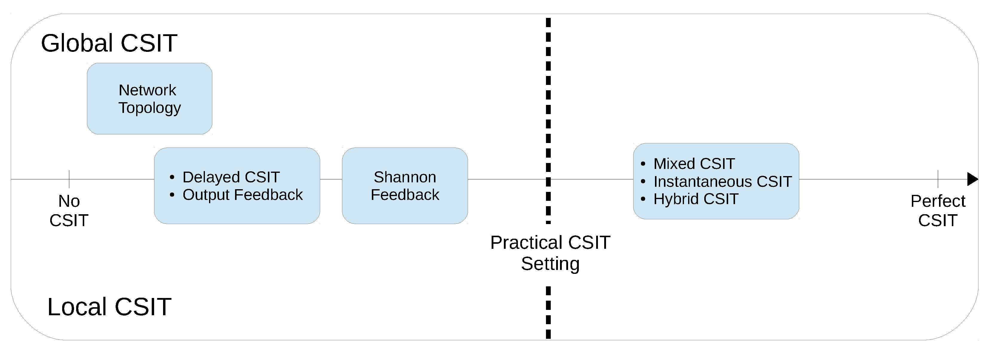
Channel state information (CSI) refers to the knowledge of channel properties of a wireless network. We differentiate between channel state information at the transmitter and at the receiver (CSIT and CSIR). CSIT and CSIR specify at which nodes (source or destination) CSI is available. Particularly, in most practical applications, it is more challenging to obtain accurate CSIT than CSIR [24]. Thus, in the latter we will restrict our focus on the quality of CSIT assuming the availability of perfect CSIR. Channel properties as part of CSIT may include but are not limited to channel coefficients in various forms (instantaneous, delayed, etc.), network topology, output feedback, etc. In the remainder of this section, we will explain various channel properties in greater depth in a specific order. That is, we aim to categorize CSIT qualitatively from high to low fidelity. Figure 1 intends to order the CSIT qualitatively.
4.1. Perfect CSIT
When transmitter node is aware of a set of instantaneous channel coefficients prior to sending symbol at time instant t, we say that this particular node possesses perfect CSIT. Specifically, when the aforementioned knowledge set of channel coefficients at node j is restricted to
- (a)
- ,
- (b)
- ,
then the j-th transmitter has access to (a) local and (b) global CSIT. Through any type of instantaneous, perfect CSIT, the transmitter can adapt its transmission strategy through adjustment in rate and/or power [25]. The majority of existing work on determining information theoretic capacity, or even capacity-approximating metrics for that matter, take the availability of perfect (global) CSIT as basis of establishing lower (achievability schemes) and upper bounds. Optimality results for this CSIT-setting can be considered as the benchmark/upper bound for any other relaxed form of CSIT to be described in the sub-sections to come.
4.2. Imperfect CSIT
By accounting for imperfections in channel estimation through piloting, feedback delay and quantization noise, the CSIT model of Section 4.1 moves to a more practical model of imprecise or imperfect CSIT. Depending on whether channel variation is small/large (fast vs. slow fading) relative to the incurred delay in CSI reporting, accuracy may vary. On the one extreme, CSI reports may be correlated with the actual channel realization of the j-th transmitter such that CSI reports represent estimation sources for imperfect instantaneous CSIT. On the other extreme, when CSI reports and are uncorrelated, channel state reports at Tx-j are outdated or delayed. The context of global and local CSIT is also applicable to the case of imperfections.
4.2.1. Imperfect Instantaneous CSIT
As described above, CSI reports to a transmitter may function as sources to estimate the instantaneous CSI at time instant t in an imperfect manner according to [26]
where and represent estimate and estimation error, respectively. For the sake of simplicity, the stochastic processes and , are assumed to be stationary and ergodic (cf. [27,28]) such that its stochastic moments do not change over time, e.g., the mean square error (MSE) becomes time-independent. For any channel , the non-negative parameter can be introduced as the power exponent of the estimation error in the high SNR regime [28,29]
We observe that every MSE scales with . Thus, for and , the estimation error scales according to and , respectively. In the first case, instantaneous CSIT estimates are error-prone and thus become obsolete whereas in the latter case, instantaneous CSIT estimates are as good as perfect in DoF sense (cf. [30]).
4.2.2. Delayed CSIT
As mentioned before, in fast fading channels CSI reports may only reveal the past channel observations. If this is the case, we term the type of CSI at the transmitter as outdated or delayed CSIT. One way of modeling delayed CSIT is similar to (10) by introducing power exponents of delayed estimation terms (e.g., [13]). The other way, a more progressive approach, is to assume that such that delayed CSIT is at least perfect in DoF sense (e.g., [11]).
4.2.3. Mixed CSIT
The class of channels where imperfect instantaneous and delayed CSI is conveyed to the transmitter is referred to as mixed CSIT model. In this regard, delayed CSI may according to Section 4.2.2 be of either perfect or imperfect quality. A mixed CSIT model with perfect or imperfect delayed CSIT is for instance applied among others in [13,31,32], respectively.
4.3. Alternating CSIT
The CSIT models of previous Section 4.1 and Section 4.2 implicitly assume that CSIT does not vary over time. Relaxing this assumption, e.g., CSIT at distributed transmitters may change from perfect (P) to delayed (D) to no CSIT (N) over time in an arbitrary order, leads to the case when multiple transmitters experience distinct time intervals with symmetric or asymmetric CSIT in an alternating fashion. In general, this type of CSIT is termed alternating CSIT [9]. For the special case of CSIT alternating between perfect instantaneous and delayed CSIT, the term hybrid CSIT is frequently used [33,34].
4.4. Feedback
Feedback, at least in case of frequency division duplex (FDD), is intrinsically coupled with CSIT transfer from receivers to transmitters. From this viewpoint, some existing works consider the impact of feedback, sometimes in addition to delayed CSIT, on the performance of distributed networks. In the literature, there are apart from CSIT reporting two main feedback models. The first feedback model is output feedback in which (a) channel output(s) become available at source nodes j with a delay of one channel use via a noiseless feedback link (cf. [35]). The term Shannon feedback is widely used when transmitters have access to both delayed CSIT and output feedback [36]. In analogy to local and global CSIT, we may distinguish between local, sometimes partial, and global feedback. In the latter, each transmitter is provided with the channel outputs of all receivers, whereas in the former, a single receiver exchanges its output with its paired transmitter. Thus, in the context of local feedback the assumption is typically to consider unique transmitter-receiver pairs for and .
4.5. Network Topology
We recall that through access to channel properties described in Section 4.1, Section 4.2, Section 4.3 and Section 4.4, the transmitters had either direct or indirect (im)perfect access to channel realizations in local or global form. A far more restrictive assumption on CSIT is when transmitters have no knowledge about channel gains except of network topology. Having access to network topology refers to knowledge about channel connectivity, i.e., knowing all channels whose impairments cause transmission signals to be received at destination nodes either in no outage or in outage.
5. Robust Schemes
In this section, we will outline the main ideas behind robust schemes applicable to relaxed CSIT assumptions through some examples. We will reference existing works for greater detail on each scheme.
5.1. MISO Broadcast Channel
In this sub-section, we will analyze the effect of CSIT on the (G)DoF through examples of the D-user multiple-input single-output (MISO) Gaussian broadcast channel (BC) that consists of S antennas, where . This is a special case of the channel model from Section 2 for S cooperating transmitters, relays and D destinations. For this particular channel, the DoF is known for specific instances of CSIT. In case of perfect CSIT, the DoF is [37,38], while for delayed CSIT the DoF of the MISO BC when corresponds to [11]. In case of mixed CSIT, is the optimal DoF of the two-user MISO BC () [27,28]. DoF-optimality for the alternating CSIT setting on the two-user MISO BC has been established in [9].
To allow for a concise presentation of existing results for various forms of CSIT, we restrict our focus to the MISO BC that consists of two transmit antennas and two single antenna receivers () (cf. Figure 2). Throughout these sections, we let and denote symbols that are independently encoded from Gaussian codewords that are intended for receiver (Rx) 1 and 2, respectively. Furthermore, represent so-called common symbols which are desired by both receivers. In a naive TDMA scheme, to avoid interference, symbols and are distributed over orthogonal channel uses such that a is attained. The following sections to come convey the main ideas of achievable schemes for distinct CSIT models (perfect, delayed CSIT, etc.) that outperform TDMA.
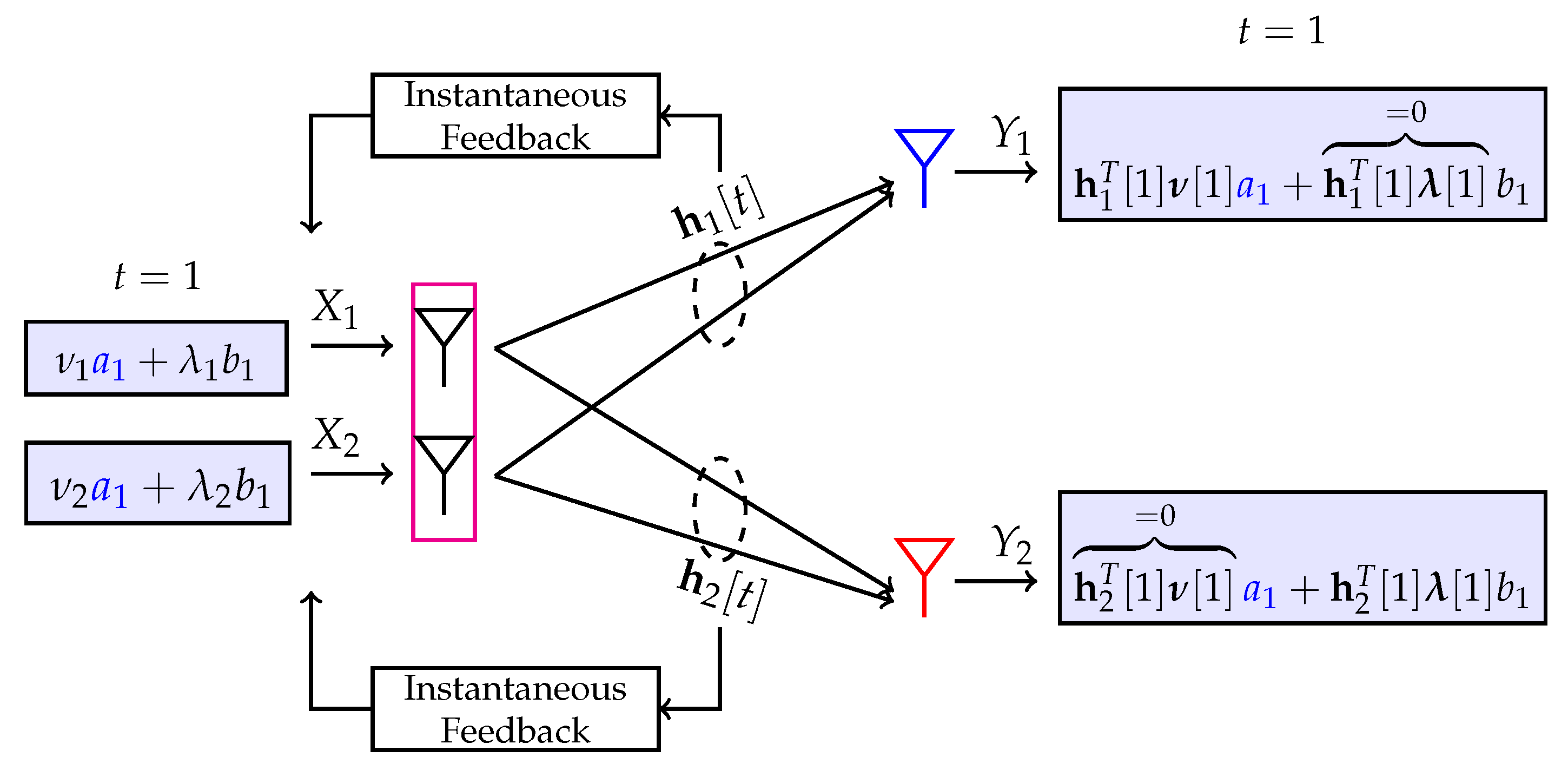
5.1.1. Perfect CSIT
In case of perfect CSIT, it is possible to attain the optimal [37,38,39], i.e., two Gaussian encoded symbols and are transferred to Rx-1 and Rx-2 in a single channel use (e.g., ). This is done by zero-forcing (ZF) beamforming of unit norm precoding vectors and at time instant such that the contribution of undesired symbols at both Rx-1 and Rx-2 is canceled (cf. Figure 2). E.g., the contribution of undesired symbol at Rx-1 is canceled by chosing the beamforming vector of to be orthogonal to the channel vector . Similarly, is set to be orthogonal to . Fixing beamformers to satisfy the orthogonality conditions
requires instantaneous CSI at the transmitters. This transforms the MISO BC into two parallel Gaussian point-to-point channels with equivalent channel coefficients and where each channel attains a DoF of 1 [40].
5.1.2. Delayed CSIT
In [11], the authors develop an optimal scheme, commonly referred to as Maddah-Ali-Tse (MAT) scheme, applicable for MISO BC’s under delayed CSIT. In their work, they show that MAT offers significant DoF gains over the setting of no CSIT. For the sake of simplicity and clarity, we restrict the focus to the two-antenna, two-user MISO BC. Figure 3 illustrates the underlying MAT scheme in two variants. The scheme assumes a time varying channel model where the channel matrix is an i.i.d. process over time and across the receivers. The channel matrix is assumed to be conveyed error-free to the transmitter in a delayed fashion at time instant t. and are Gaussian symbols intended for receiver (Rx) 1 whereas and are desired by Rx-2. Through the MAT scheme these four symbols are conveyed to the receivers in three channel uses attaining the optimal . The transmission scheme consists of two phases in total and variant one for instance works as follows:
- In the first phase consisting of two channel uses ( and in Figure 3a) the transmitter broadcasts symbols and in and and in . Thus, the received signal at Rx-1 and Rx-2 are (noise-corrupted) linear combinations of and the respective channels at , i.e.,as well as linear combinations of at given by:Thus, channel use is used to serve Rx-1, while channel use is utilized to serve Rx-2. Specifically, this means that received signals and are overheard signals at Rx-2 and Rx-1, respectively. These two overheard signals do not provide the respective receivers with useful information on their desired symbols. However, the i.i.d. assumption in the channel matrixfor arbitrary t implies that is of full rank almost surely. This suggests that the overheard signal of Rx-2 is an independent observation in Rx-1’s desired symbols and than the signal . The same relationship applies to and . In DoF sense at which SNR is asymptotically large, it suffices to restrict the focus on overheard equations and (that are free from noise) instead of overheard signals and . Since every receiver seeks to decode two symbols, either or , each receiver needs two independent observations as a function of its desired symbols. Specifically, for these two receivers this means: If Rx-1 is aware of and Rx-2 of , decoding of and at the respective receivers becomes feasible within bounded noise distortion. Recall that and are yet unknown to receivers 1 and 2 from channel uses and . Consequently, in phase two, the goal is to convey to Rx-1 and to Rx-2. In phase two, delayed CSIT comes into play when locally constructing overheard equations at the transmitter.
- In phase two, the overheard equations and are conveyed to their desired receivers in the single channel use . At time instant , the transmitter is aware of both and since it has access to delayed CSIT. Therefore, the transmitter can generate overheard equations and at time instant . By sending the common symbolfrom a single antenna element allows each receiver to use its side information and obtain the overheard equation of the complementary receiver. E.g., when sending , Rx-1 uses the knowledge of the overheard equation as side information and CSIR to cancel its contribution from . By doing so, Rx-1 retrieves from . Thus, Rx-1 now possesses two (noisy) linear independent equations in enabling Rx-1 to decode its desired symbols within bounded noise [41].
With the MAT scheme, we were able to transmit two desired symbols to both Rx-1 and Rx-2 in three channel uses. This equals a DoF of . In variant two of the MAT scheme, a linear combination (similarly to Figure 2) of all four symbols is conveyed to the receivers. Thus, this changes the transmission scheme in channel uses and in so far as the interferences that Rx-1 () and Rx-2 () perceive at time instant are locally constructed at the transmitter (through access to delayed CSI ) and are broadcast. These interferences have a dual purpose: (a) Either they are utilized to cancel interference observed at in retrospect or (b) they provide the receiver with an additional observation on its desired symbols. Through this variant, each receiver obtains two independent observations as a function of its two desired symbols enabling succesful decoding almost surely. We observe when constructing interferences at the transmitter, variant two only utilized CSI , whereas variant one both and . Further details on the generalized achievability scheme and converse arguments for various number of users and transmit antenna elements on the MISO BC are available in [11].
Extension of this seminal work study a variety of networks, namely two-user multiple-input multiple-output (MIMO) broadcast channels [12,42,43,44] and (MIMO) interference channels [45,46,47], Z-channels [48], X-channels with [35,36] and without feedback [49,50], and with secrecy constraints in [51].
5.1.3. Mixed CSIT
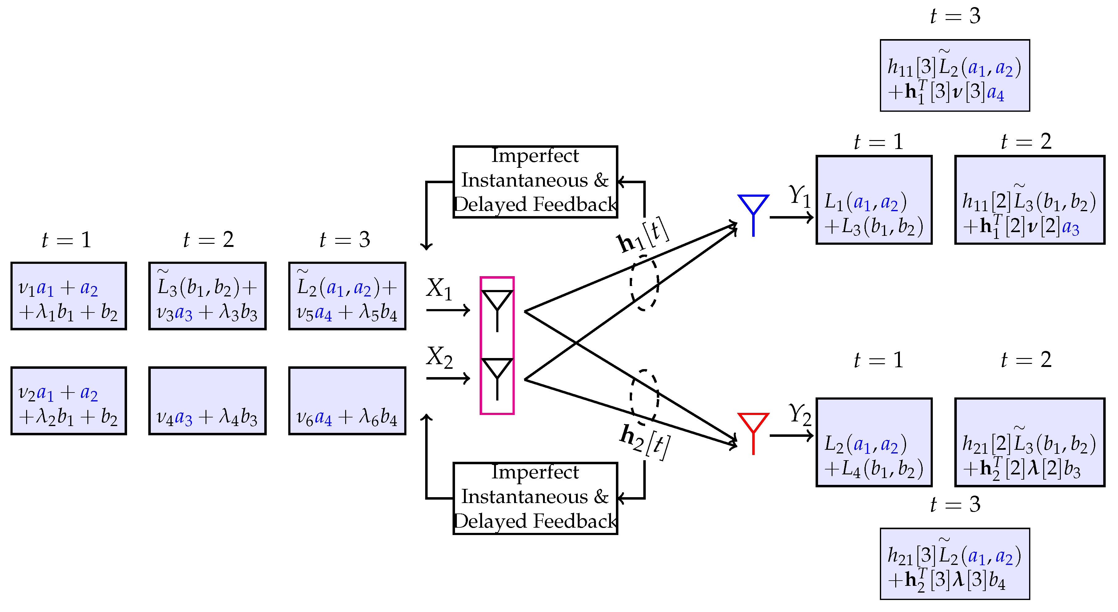
In this section, the benefits of having transmitters with simultaneous access to delayed and imperfect instantaneous CSI, i.e., mixed CSIT, is outlined on the aforementioned MISO BC example. We will see that for this setting, synergistic benefits of instantaneous and delayed CSIT is utilized efficiently by combining zero-forcing beamforming and a modified MAT scheme. This observation becomes clear when comparing Figure 2 and Figure 3b with the proposed scheme for mixed CSIT shown in Figure 4.
First, let us explain the ZF part of this scheme. Let us recall that transmitters have only estimates of instantaneous CSIT. At all time instants and , the transmitter conducts zero-forcing beamforming by exploiting its imperfect instantaneous CSIT similarly to (12), by exploiting its CSI estimates as follows:
However, since instantaneous CSIT is of imperfect quality, zero-forcing beamforming can only partially zero-force interfering symbols at unintended receivers. The orthogonality condition in Equation (19) ensures that through ZF the (expected) power level of interfering symbols reduces by factors of
Hereby, step follows by assuming that the CSIT quality parameters (cf. Equation (11)) are identical for all channels in . Thus, the power level of symbols that are (partially) zero-forced ( at Rx-1 and at Rx-2) reduces by (cf. Figure 5a vs. Figure 5b,c). For instance, symbol is transmitted in channel use at the highest transmit power level P (see Figure 5a) and is received at the intended receiver Rx-2 without any change in power while it is partially zero-forced to a power level at the unintended receiver Rx-1 as illustrated in Figure 5b,c for . On the other hand, when conveying symbols and in channel uses and , a lower transmit power is allocated to each symbol, that is only (cf. Figure 5a for and ), such that these symbols are zero-forced at Rx-1 to the noise power level of ; thus, being completely negligible in DoF sense. Due to symmetry, the same observation holds true for symbols and with the slight difference that the roles of the receivers swap. Symbols and , on the other hand, are not precoded which is why their power levels do not change at either receiver and remain at . Now, we move to the MAT part of this scheme. At time instant , two precoded symbols of high power P () and two symbols of lower power () are sent to the receivers. Thus, the receivers observations become:
As already mentioned, out of these four symbols only the symbols of higher power ( and ) are partially zero-forced to power levels of at their unintended receiver; thus, enabling that the power level of the zero-forced symbol is in agreement with the power level of symbols and . We conclude that the power levels of residual interferences and correspond to . Similarly to the MAT scheme illustrated in Figure 3b, both receivers can recover their desired symbols if these two residual interferences become available at both receivers. Consequently, we would like to convey them to both receivers in channel uses and . Unlike the MAT scheme, however, where these interferences are transmitted in an analog fashion, this scheme quantizes them prior to transmission. The reason for this lies in the fact that in contrast to the original MAT scheme where ZF was infeasible (due to restriction to delayed CSIT) this scheme reduces the power level of residual interferences to . Thus, it is possible to compress the interferences allowing for the simultaneous transmission of new symbols in and in (all of which are of power ). The benefits of digitizing the interferences over an analog solution becomes particularly significant when CSIT is close to perfect, i.e., close to . In this case, there is a mismatch between available transmit power being at P and residual interference power being close to noise power . Therefore, quantizing residual interferences is preferable to analog solutions. The number of quantization bits depends on the interference power and the average target distortion D [40,41,52]. We quantize the residual interferences according to:
where and , respectively, are the quantization values and quantization noise terms with average distortion . In DoF sense, the quantization noise becomes negligible if we set the target distortion to
According to ([40], Chapter 10), the rate of the quantized components under above distortion measure becomes
In channel use , along with symbols is provided to the receivers, while in symbols are utilized. The decoding of all these symbols is conducted as follows.
- After decoding of and , the receivers can remove the contribution of the decoded signals and retrieve their desired symbols, i.e., at Rx-1 and at Rx-2.
The resulting DoF, achievable in 3 channel uses thus becomes
A plot of the achievable DoF for the described scheme, ZF, TDMA, MAT and a suboptimal scheme by Kobayashi et al. [29] are shown in Figure 6. We see that the optimal scheme contains the optimality of MAT for delayed CSIT only () and ZF for perfect CSIT (). We mention for the sake of completeness, that the DoF collapses to that of TDMA, i.e., to 1, for all CSIT settings with finite precision where probability density functions of unknown channel realizations are bounded and do not scale with P [58].
5.1.4. Alternating CSIT with Fluctuating Topology
We now consider an alternating CSIT setting for the MISO BC with unequal channel strengths for and , . Through this model, we gain insight on how CSIT feedback policies that provide the transmitter with either perfect (P), or delayed (D) or even no CSIT (N) over time affects achievable rates from a GDoF perspective. To this end, we modify the signal model at both receivers, similarly to Equation (8), to:
where we used
in aforementioned equation. We recall that through this modified model, the power constraint at the transmitter is bounded by unity where effective channel coefficients of Rx-1 and Rx-2 now become and , respectively. Importantly, the large-scale fading effect of these coefficients (), are time-varying; thus, making the topology of the MISO BC fluctuating in signal strength. In addition, to capture alternating CSIT, we define indicator variables to denote which one of the CSIT states or N for time t, Rx-1 and Rx-2 feed back to the transmitter. For instance, Figure 7a illustrates the system model for state . When considering an entire transmission interval spanning multiple channel uses, the transmitters are interested in knowing the fraction of the transmission time (a) during which the CSIT state is given by any pair [9] and (b) during which the topology state is given by any pair [62,63]. Thus, effectively, and correspond to two-dimensional probability mass functions that depend on the pair of random variables and , respectively [64]. In the sequel, we characterize how the achievable GDoF is affected when CSIT is available according to:
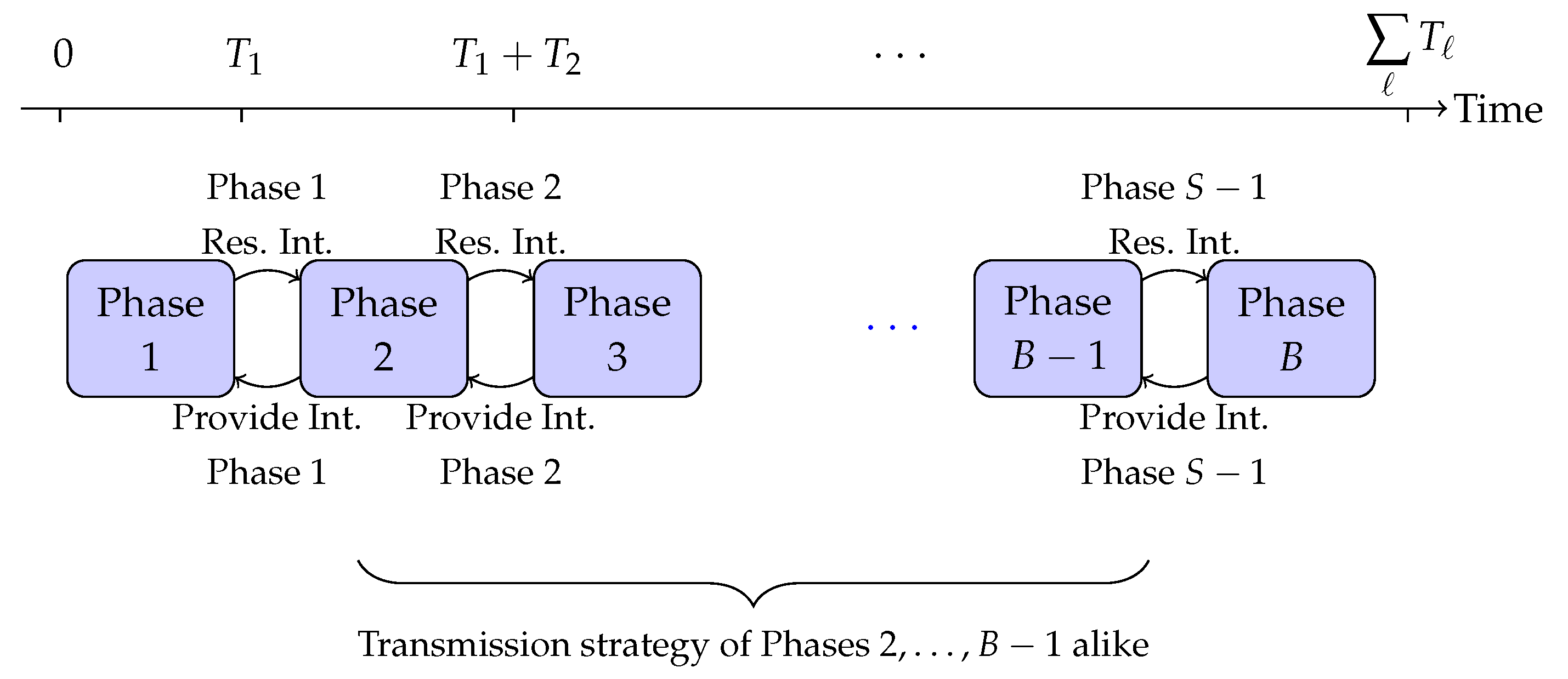
We now highlight the main aspect of the coding scheme that is applicable to examples (a) and (b). Generally, the scheme is composed of B communication blocks in a block-Markov fashion [65,66], where the length of every block is restricted to a finite, constant number of channel uses. In all blocks , we convey the receivers with private and common information. To be more precise, in every block ℓ newly encoded information symbols are transmitted as private information, while residual interference (observed at the receivers in the previous block are locally constructed through the transmitter’s access to delayed CSIT, quantized and finally) is transmitted as common symbols to the receivers. In the last block, however, the transmitter sends only common symbols to Rx-1 and Rx-2. At the receivers, the decoding starts from the last block and moves backward. Specifically, common information of the ℓ-th block is used to decode both private and common symbols of the ()-th block.
Let us now move to example (a). In this example, the network topology is fixed to the static setting, i.e., . In (G)DoF sense, this means that the channel to Rx-1 is stronger than the channel to Rx-2 since the former channel supports a DoF of at most 1 while the latter only a DoF of at most . Furthermore, the CSIT state and occur all at the same frequency. For instance, in a block of channel uses, the CSIT states may occur periodically according to:
For arbitrary , (32) is generalized to:
We proceed to describe (i) encoding, (ii) creation of common symbols and (iii) decoding for an arbitrary block ℓ, of CSIT sequence (33). Particularly, when explaining the creation and transmission of common symbols, we will need to make adjustments on how long of a fraction we will actually make use of delayed CSIT. This will be captured by the parameter n as we shall see later. For the sake of notational simplicity when referring to the i-th channel use of block ℓ, we use the notation to refer to this time index. In most cases, however, we are referring to a specific block, which is why we drop the block-time indexing notation and simply write t to refer to time instant .
(i) Now, we start with the encoding. In the sequel, we focus on the ℓ-th block if not otherwise stated. The transmission signal (with some abuse of notation) for this block is
where a and b are private information symbols intended for Rx-1 and Rx-2, respectively, where is a common symbol. The intuition behind the choice of Equation (34) is as follows:
- With the use of private symbol , we account for the fixed -topology (TP). Concretely, due to its scaling with , this symbol is received at power level at its intended receiver Rx-1, whereas it is received at noise level at its unintended receiver Rx-2. Being received at noise level at Rx-2, makes it a negligible interference term in (G)DoF sense.
- Depending on whether the CSIT state or is present, we can improve the achievable rate of the user with no CSIT feedback by utilizing the general idea of the MAT scheme. That is, we can create interference at the unintended receiver as side information which can be canceled in retrospect through the use of delayed CSIT while providing the intended receiver with additional information on its desired symbols. For instance, in state , we send among others and , which creates interference at Rx-1, but represents desired information for Rx-2. Constructing, the observation of Rx-1 in terms and locally at the transmitter and broadcasting this information, will help Rx-1 canceling interference and provide Rx-2 with extra information for decoding and .
- In state , it is advisable not to send any additional private information. This is simply because private information represents interference to one of the two receivers which cannot be reconstructed (and thus canceled) due to the lack of CSIT.
With above expression on , the received signal at both receivers under a static -topology () becomes (cf. Equations (29) and (30))
(ii) Identical to the scheme introduced for mixed CSIT, interference that occurs at Rx-1 in CSIT state
as well as interference at Rx-2 in CSIT state
can be quantized locally due to availability of delayed CSIT to and with approximately and quantization bits, respectively (The term “approximate” is used whenever we avoid explicitly specifying the missing quantization bits. These bits, however, are negligible in (G)DoF sense since when .).
Over each block ℓ, , spanning channel uses, the approximate total number of quantization bits is
These quantization bits of block ℓ are then mapped into common information symbols that are transmitted in the consecutive block . For reliable decoding, this necessitates that the achievable rate of conveying common symbols in block is at least equal to the number of quantization bits given in Equation (39).
(iii) The per-block decoding of the ℓ-th block, , relies on successive decoding. Initially, the common information of block is used to reconstruct and at both receivers. Through and interferences in distorted signals for state and in Equations (35) and (36) at Rx-1 and Rx-2 are removed, respectively. The decoding order of the remaining desired symbols at the receivers are given by
for any t formed by the block-time indexing notation . Common symbols are decoded through TIN, allowing for decoding at a per-block sum rate of
where step (a) enforces that the achievables rates at both receivers become identical by equating the time duration in operating in states and . After removal of , Rx-1 and Rx-2 decode their remaining desired symbols as follows. Rx-1, on the one hand, applies TIN and decoding as in MIMO on its received output signals in their noiseless form
to decode all at a per-block (sum) rate of
as well as all at a per-block rate of
Rx-2, on the other hand, applies MIMO decoding on its received output signals in their noiseless form
to decode all at a per-block (sum) rate of
By choosing n, i.e., the number of channel uses in and state operation, we ensure the decodability of common symbols for every block ℓ. Recall that for this condition to be satisfied the achievable rate of conveying common symbols in block has to be at least equal to the number of quantization bits given in Equation (39), i.e.,:
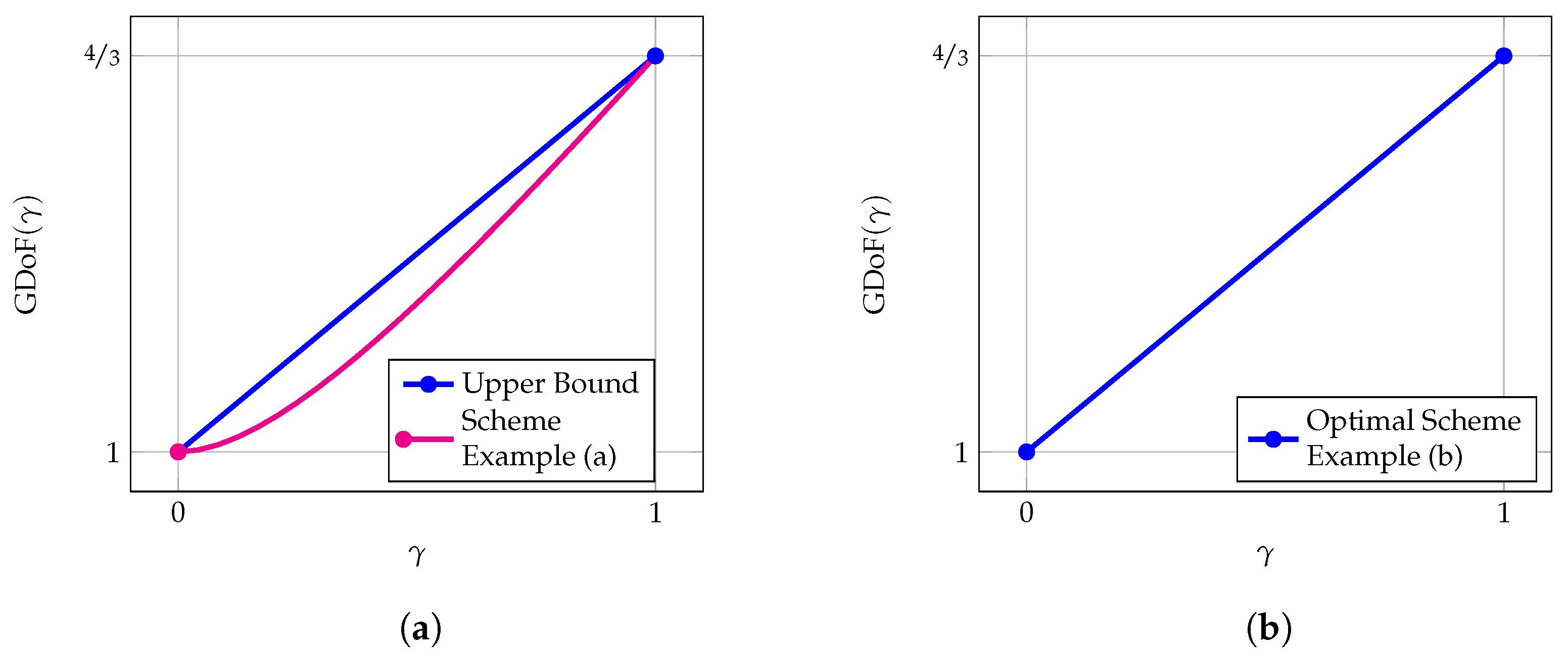
The rate is maximized if we choose n to be as large as possible. This is achieved if . Concretely, this means that for a given -topology with , we actually only operate in the and states for a fraction of of block length . With the achievable rates known, we can now compute the achievable GDoF to:
Now we consider example (b). In this example, the network topology is symmetrically fluctuating between a and -topology () where at every time instant both receivers provide the transmitter with delayed CSIT information. In a single block () of channel uses, the topology states may occur according to:
Under this particular sequence of topology states, we will focus on the first half of the block spanning channel uses (comprising of topology states ) to formulate the achievability scheme. For the remaining uses under the complementary topology state, the scheme follows along the same lines of argument requiring minor modifications. We proceed to describe details of the scheme for the first channel uses.
The transmission signal at time instants is set identically to that of the MAT scheme variant one (cf. Figure 3a) which is:
Under this transmission signal, the received signals at both receivers under a fluctuating topology given by (42) for correspond to:
Similarly to the MAT scheme, interference that occurs at Rx-2 in TP state in
as well as interference at Rx-1 in TP state in
can be locally constructed through the use of delayed CSIT. Also as in the MAT scheme, exploiting side information of the receivers, it suffices to broadcast the sum of and to the receivers (Recall that Rx-1 knows a noise-corrupted version of while Rx-2 is aware of a noise-corrupted version of .). As opposed to the MAT scheme, however, it is advisable to quantize the sum of these interferences to requiring approximately quantization bits for this signal. The quantized signal functions as a common signal since it is desired by both receivers. Thus, at , where a -topology is present, we send in addition to according to
The reasoning behind the transmission of in addition to the common symbol is identical to the justification of using it in example (a). The received signals at both receivers are given by
It is straightforward to see from Equation (49), that Rx-1 can apply successive decoding to first decode at an approximate rate of and then decode at a rate of approximately . Rx-2, on the other hand, effectively observes a point-to-point channel in (50) for which reliable decoding of is feasible at a rate of . By knowing , Rx-1 and Rx-2 obtain the MIMO observations
respectively. In these two equations, we have neglected additive noise terms (including quantization noise). These effective MIMO channels allow for decoding of and at approximate sum rates of , respectively [67]. The GDoF as a function of can easily be computed to
A direct comparison of achievable rates for examples (a) and (b) with upper bounds on the GDoF [62] is shown in Figure 8. It can be seen from Figure 8b that only the scheme for example (b) is optimal for arbitrary . We conjecture that the suboptimality of scheme for example (a) is due to the suboptimal creation and transmission of common symbols .
5.1.5. Conclusion: MISO Broadcast Channel
In this section, we have introduced various schemes that are applicable for CSIT of distinct qualities. We used DoF and GDoF metrics as first-order approximations of sum rates. Particularly, we have seen that outdated CSIT is useful in recreating interferences and allowing for retrospective interference cancelation. When the transmitter in a MISO BC becomes also aware of imperfect instantaneous CSIT in addition to delayed CSIT, it is possible to synergestically apply optimal schemes for perfect and delayed CSIT, that is MAT and ZF scheme, in an appropriate manner. In conclusion, interference management for MISO BC’s in case of imprecise CSIT is well-established but requires further research, among other finding topology-aware optimal schemes for alternating CSIT configurations. As we move to distributed interference networks (interference channel, X-Channel, etc.), interference management for imprecise CSIT is far less understood in achievability and converse sense [69,70].
5.2. Distributed Interference Networks
In distributed wireless networks, where there is no cooperation among source nodes, the paradigm of handling interference changes from removing interference to aligning interference [7]. For instance, when ZF precoding that precancels interference was optimal for the MISO BC [37], interference alignment has been shown to achieve the optimal DoF for a variety of distributed wireless networks [4,6,8,71,72]. The idea of interference alignment (IA) is to lessen the effect of interference by merging the communication dimensions occupied by interfering signals. In [4], Cadambe and Jafar showed, contrary to the popular belief, that interference alignment attains the optimal DoF of the D-user interference channel (IC), , with single antenna nodes and a time-varying channel. Under identical assumptions, the same authors extend their results on the D-user IC channel to the X-channel for which they show the optimal DoF to be [8]. For constant channels, where conventional vector alignment [4,8] fails in attaining the full DoF, interference alignment along rationally independent dimensions, so-called real interference alignment [73,74] proves useful. In [75], Motahari et al. showed that through real interference alignment the total DoF for both D-user IC and X-channel are achievable even for real, time-invariant channels. For the majority of these networks, however, the main caveat behind these schemes is that the optimal DoF is only achieved asymptotically either through infinite channel uses in case of vector alignment or infinite transmit directions in case of real interference alignment.
Besides, implementation of interference alignment requires transmitters to have access to global CSIT. As we relax the CSIT assumption, interference management is rather poorly understood compared to broadcast channels. For instance, even for the X-channel under delayed CSIT, DoF optimality is yet restricted to linear schemes [70]. In addition, the DoF loss incurred for distributed wireless networks when moving away from perfect CSIT can be significant. For instance, for the best known scheme on the D-user IC under delayed CSIT [50], the DoF converges to the constant (i.e., it does not scale with the number of users) which is in stark contrast to the optimal DoF of under perfect CSIT. On the contrary, the scaling of the DoF with the number of users D is maintained in MISO BC’s where the DoF is shown in [11] to be . Ultimately, it is highly desirable to maintain a DoF close to what was achievable under perfect CSIT as CSIT requirements are relaxed. In Section 5.2.1, we illustrate through an example that under mixed CSIT and partial output feedback, robust interference management is feasible.
For many multiuser networks, relaying operation is beneficial in improving achievable rates [65,76,77,78,79,80,81]. From a DoF-perspective, however, relaying has been shown in [82] to provide no additional DoF gain for the fully connected IC and X-channel with full CSI at all nodes. In this regard, the fundamental question boils down to whether relaying is capable of facilitating interference alignment at all. Existing works [83,84,85] answer this question in the affirmative by revealing strategies of how relays can be utilized to transform a static channel into an equivalent time-varying channel such that full DoF is attainable through interference alignment. In [86], Ning et al. presents a relay-aided interference alignment scheme that results in the optimal DoF of the D-user interference channel with finite channel uses. We recall that traditional IA without relays required infinite channel uses/transmit directions for the D-user IC for and the X-channel for and [4,8].
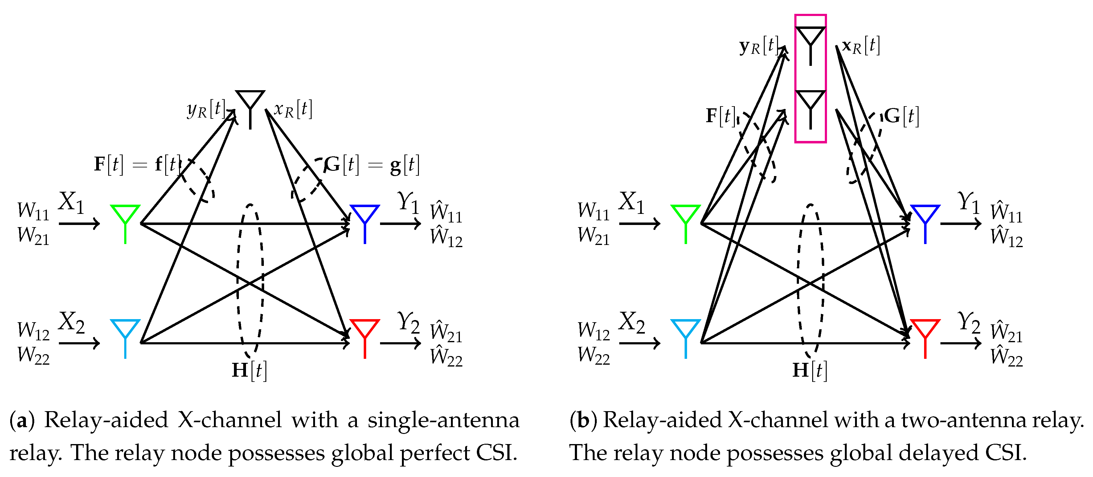
Interestingly, relays do not only facilitate interference alignment but can also lower CSI requirements at the transmitters. In Section 5.2.2, we will outline two examples of an X-channel on how relays can effectively assist blind transmitters, i.e., transmitters that completely lack CSI, in achieving either full DoF or at least a DoF that scales with the number of users. Hereby, the X-channel is a special case of the channel model from Section 2 for transmitters and destinations. Specifically, in this network Tx-j, , has a message for Rx-i, . Furthermore, denotes the codeword of message . In brief, in example (a) depicted in Figure 9a, a single-antenna, half-duplex relay () has perfect CSI and assists the blind transmitters Tx-1 and Tx-2 in achieving the full of the X-channel through interference alignment. Further, in example (b) depicted in Figure 9b, on the other hand, cooperating half-duplex relays (i.e., a single half-duplex relay with two antenna elements) have only delayed CSI and aid the blind transmitters Tx-1 and Tx-2 in achieving the optimal through a MAT-related scheme.
5.2.1. X-Channel with Mixed CSIT and Feedback
We consider the X-channel illustrated in Figure 10 as an example of distributed networks under mixed CSIT (and partial output feedback). Similar to Section 5.1.3, where we described a robust scheme on the MISO BC under mixed CSIT, the scheme on the X-channel will, in addition to the output feedback provided to Tx-3, exploit mixed CSIT at all transmitters by facilitating partial ZF possibilities. Specifically, as shown in Figure 11, the coding scheme is composed of a multi-phase transmission strategy, where in every phase, information about delayed and current CSIT is used to form precoding scalars that diminish the effect of interfering symbols at the two receivers. Since the instantaneous CSIT is of imperfect quality, it is in general not possible to fully remove interference at a particular phase of the coding scheme. Due to the availability of delayed CSIT, the remaining residual interference of each phase is encoded as common information that is transmitted along with new private symbols in the consecutive phase. Common information is decoded by TIN (treating interference as noise), i.e., by treating private information as noise. The transmission scheme terminates if no more interference is observed at either receiver. At the end of the transmission, symbol decoding is performed through retrospective interference cancellation of interference-distorted signals.
We now highlight the main aspect of the coding scheme that consists of B phases, where the time duration of each phase ℓ is restricted to channel uses. With the exception of phase 1, in all remaining phases , we convey the receivers with private and common information. To be more precise, in every phase ℓ newly encoded high powered information symbols and low powered symbols are transmitted as private information, while residual interference (observed at the receivers in the previous phase are locally constructed at Tx-3 through the transmitter’s access to partial output feedback and delayed CSIT, quantized and finally) is transmitted as common symbols to the receivers. In the last phase B, no residual interference is observed at both Rx-1 and Rx-2. Thus, at the receivers the decoding starts from the last block B and incrementally moves backward. Specifically, common information of the ℓ-th phase is used to decode both private and common symbols of the ()-th phase.
For the sake of simplicity, we proceed to describe (i) encoding, (ii) creation of common symbols and (iii) decoding for phase 1 (). The transmission strategy of the other phases are similar to with differences in the power allocation of high power and low power information symbols. Further details on these phases are provided in [32]. For the sake of notational simplicity, we stack the transmission signals of all three transmitters to a three-dimensional vector .
Now, we begin with (i) the encoding of phase . Phase 1 is composed of sub-phases, where each sub-phase consists of 4 channel uses. We will only focus on the first sub-phase. The remaining sub-phases will simply be a repetition of the first sub-phase, with each sub-phase corresponding to new information symbols. In the first sub-phase, 6 high power information symbols of power order P and 4 low power symbols of order are transmitted. The channel inputs are given by
where and denote the precoding scalars of information symbols a and b, respectively. How these scalars are chosen will be specified in the paragraph to come. Under this choice of transmission signals for , the i-th receiver’s channel outputs (neglecting noise) become:
For Rx-1 (Rx-2), () is information on its desired symbols while () represents interference side information. The side information can be used to subtract the contribution of Rx-1’s (Rx-2’s) undesired symbol () from its outputs () at channel uses 3 and 4, respectively. This operation at Rx-1 and Rx-2 is accounted for by the post-coding matrices and , respectively:
Under the given post-coding matrices, the two receivers observation become:
The receivers signals’ after post-coding (cf. Equations (56) and (57)) are composed of a sum of two parts, a desired and an undesired part. The undesired part represents residual interference that is originating from Tx-2 and Tx-3 only. We exploit the knowledge in mixed CSIT in the choice of the precoding scalars and such that the power levels of residual interferences at Rx-2 and Rx-1 are minimized. To this end, we fix, for instance, and to
so that the power levels of residual interference components (in Equations (56) and (57))
associated to high powered symbols reduce to the same power levels of the interference imposed by low powered symbols (which is ). For further details on the power reduction, we relegate the reader to Section 5.1.3 of this survey. The remaining precoding scalars are chosen similarly to and . Through this choice in precoding scalars, each residual interference component has a power level of so that the overall power level of residual interference is also in the order . Next, (ii) the creation of common symbols is described.
Output feedback provides Tx-3 with 4 equations that depend on 10 symbols. As Tx-3 has access to delayed CSIT and local knowledge of 6 symbols (), it can remove the contribution of these symbols in . Thus, delayed CSIT and output feedback from Rx-1 to Tx-3, enables Tx-3 to decode symbols available at Tx-1 and available at Tx-2 after 4 channel uses almost surely. Hence, the third transmitter knows all symbols of phase 1 and is therefore capable to generate all 4 residual interferences given in Equations (56) and (57) locally. The residual interferences available at Rx-1 (Rx-2) are a function of symbols desired by Rx-2 (Rx-1). Hence, conveying these interference components as common information is beneficial to both Rx-1 and Rx-2 in a sense that, it provides extra equations to Rx-2 (Rx-1) to decode its desired symbols; and, in doing so, it helps Rx-1 (Rx-2) to remove the residual interferences. Recall from the previous paragraph that all residual interferences are of order . Thus, by digitizing interferences to bits is sufficient for decodability at both receivers within bounded noise [40]. Due to the availability of delayed CSIT, Tx-3 is able to construct the desired component of residual interferences digitally. As the first 4 channel uses are repeated times, the total number of quantization bits in phase 1 are then given by bits. These bits will be distributed into common symbols of the second phase (). In the next paragraph, we elaborate on (iii) the decoding of the desired information symbols.
Recall that backwards decoding is applied. For phase 1, this means that the common information conveyed in phase 2 has to be available before the receivers initiate the decoding of their desired information symbols of phase 1. With knowledge in common information the receivers are aware of all residual interferences. These residual interferences are used for interference cancelation and extra information on desired symbols. As a consequence, for any sub-phase, each receiver has 5 independent observations on 5 desired information symbols. Thus, for instance, Rx-1 can decode high power information symbols (each at a rate of bits) and low power information symbols (each at a rate of bits). Hence, the overall information content conveyed to each receiver in Phase 1 is bits.
Combining the achievable sum rates in private information of all B phases (for large B) attained in channel uses gives the resulting achievable DoF
A plot of the resulting DoF is shown in Figure 12. The plot shows that finite quality CSIT () and partial output feedback compensate for the absence of perfect CSIT. For the case of and partial output feedback, the optimal DoF of is already attainable.
5.2.2. Relay-Aided Interference Alignment for X-Channel without CSIT
In this section, we will show that symbols and desired by Rx-1 and Rx-2, respectively, are conveyed reliably to their intended receivers in 3 channel uses (corresponding to the optimal ). From an individual receivers’ perspective this means that 2 out of 3 available signaling dimensions ought to be reserved for desired symbols while the remaining signaling dimension is utilized to align the two remaining interfering symbols. Interestingly, for this to happen only the relay node requires either (a) full CSIT and a single antenna (cf. Figure 9a) or (b) delayed CSIT and two antennas (cf. Figure 9b) while the transmitters can be entirely blind. Generalizations of cases (a) and (b) on the X-channel are available in [19,20].
For notational convenience, we stack the transmit signals to a two-dimensional vector . In the first two channel uses, , both transmitters are active and send their symbols to the two receivers, while the relay remains silent and only listens and stores the received signals . Specifically, the transmission signal for is set to:
In what follows, we first describe the main ideas (a) for the case a single-antenna relay with access to full CSI (Figure 9a) and (b) the case of two-antenna relay with access to only delayed CSI (Figure 9b). We start with case (a).
In channel uses , the relay receives one noise-corrupted linear combination in Rx-1’s desired symbols , i.e.,
and an additional noise-corrupted linear combination in Rx-2’s desired symbols , i.e.,
So far, the receivers attain two observations. One observation depends only on desired symbols while the other observation depends on undesired symbols. For instance, (and ) is a function of and ( and ) which are (un)desired symbols of Rx-1. At the last channel use , we exploit the knowledge of the relay gained at channel uses to provide each destination with an additional observation on its desired symbols. To this end, the transmission signals at the transmitter and the relay are chosen according to:
Under the choice of transmission signals at both sources and relays, we can write the received signals at Rx-i, , for by:
Let us first describe the decoding from the perspective of Rx-1 (). For a per-user DoF of , Rx-1 has to decode and in three channel uses. This is achieved by aligning undesired symbols and into a one-dimensional signal space while allocating the remaining two signal dimensions for its desired symbols and . On the basis of (66) for , it is easy to see that and are aligned if we let the scalar satisfy the condition:
Similarly, at Rx-2 alignment of undesired symbols and is feasible for in Equation (66) if is chosen such that
Since the relay node has access to perfect CSI, and can be computed locally such that the conditions specified in Equations (67) and (68) are fulfilled. Through zero-forcing post-coding on , the receivers are able to isolate their desired symbols from the aligned interference. For instance, by fixing the post-coding matrix at Rx-1 to
its observation after post-coding is (for notational convenience, we neglect the noise term)
Analogously, at Rx-2 the post-coding matrix is
such that its observation after post-coding becomes
After post-coding, each receiver has two linear-independent observations of its desired symbols (cf. Equations (70) and (72)). This enables each receiver to decode its pair of desired symbol in three channel uses. Thus, a DoF of is attained for which we only required full CSI at the single-antenna relay.
We now move to case (b). For this case, where the relay node has two antennas, the source-relay link is a SIMO multiple-access channel [40,41] for which we can decode two symbols per channel use through ZF reliably. Thus, the relay knows all symbols after the first two channel uses. By assumption, since the relay has delayed CSI from the previous two channel uses, it can apply the same transmission approach as in the MAT scheme variant one for . That is, it exploits the side information at Rx-2 (which is ) and at Rx-1 (which is ) to multicast and . The source nodes, however, remain silent. The receivers use their side-information to retrieve a second, independent observation on its desired symbols. For instance, Rx-1 exploits its side information to obtain . Knowing and , Rx-1 is able to decode . A similar observation holds for Rx-2. Overall, for case (b), again a DoF of is achievable requiring in comparison to (a) only delayed CSIT at a cost of an additional antenna element.
6. Conclusions and Open Problems
In this survey, a thorough presentation of state-of-the-art robust interference management schemes for distributed and non-distributed Gaussian networks in case of imperfect CSIT was given. Carefully chosen examples analyzed the (G)DoF metric for various levels of imperfect CSIT including mixed (with and without feedback), alternating (with fluctuating topology), delayed and no CSIT. Gaussian codewords were utilized to show the (G)DoF optimality for these CSIT settings. In certain cases, lattice codes [87,88,89] have been shown to outperform Gaussian codewords [90]. Such comparison, however, is beyond the scope of this survey. The study of the (G)DoF for these relaxations of the perfect CSIT case has already led to important theoretical insights; however, the results obtained so far rather resemble isolated islands in the sense that transmitters have only access to one form of channel knowledge. In practice, the transmitters might have knowledge of a mixture of various forms of CSIT. In this context, we believe that the research community has to deepen its knowledge in GDoF-sense, i.e., understand the interplay between channel strengths and uncertainty levels . This research path is practically motivated due to evolution of heterogeneous networks where channels are typically unequal in strength and channel estimation quality across multiple transmitters (macro, small, femto basestations) differs. Such research will, in addition to other goals, clarify how the knowledge of channel strength (and as such the network topology) and imperfect instantaneous (as well as delayed) CSIT be utilized jointly in an optimized fashion. In addition, through this line of research, existing works on specific CSIT settings, e.g., delayed and perfect CSIT for fixed channel channel strengths, may be bridged. Wireless networks that shall be subject to this research thrust are particularly (i) (relay-aided) distributed networks and (ii) multi-way channels [91] and (iii) eavesdropper channels [92]. In the following, we will briefly outline some challenging open problems for these three channel types.
As far as (i) distributed networks are concerned little is known about the GDoF for imperfect CSIT. Recently, the interplay between channel strength and quality on the non-distributed two-user MISO BC has been fully characterized [93]. Their results show that the GDoF depends only on the weakest CSIT parameter for each receiver. Further, they develop conditions for which it is GDoF-optimal to serve only a single user. Extension of this research to distributed networks is of viable interest. Progress in this research area would enable as to how combinations of schemes, such as TIN, ZF, etc., are optimal. Even for the special case of fixed topology () and constant channel uncertainty (), it is unknown whether interference alignment and common signaling over distinct power levels is DoF-optimal.
Furthermore, (ii) multi-way channels allow for significant improvement in the spectral efficiency of wireless networks (e.g., a two-way communication channel with two users can achieve up to twice the rate that would be achieved had each user transmitted separately) [94]. For the perfect CSIT setting, the optimal DoF of various networks, among others, the MIMO two-way X relay channel [95], the K-user two-way interference channel with and without a MIMO relay [96] and the Y-channel [97,98,99] have been studied. The investigation of the DoF for the case of imperfect CSIT is almost completely unexplored with some exceptions of the achievable DoF for the Y-channel where users have either access to delayed CSI [100] or no CSI access during the MAC phase [101]. Substantial amount of work is needed in order to understand the implications of imperfect CSIT on the aforementioned performance gains of multi-way channels. This requires new upper bounds which take into account various CSIT settings.
An important aspect of future communication systems is the aspect of robustness in terms of confidentiality. In contrast to previous generations a security-by-design approach should be pursued. However, only very few works investigate the influence of imperfect CSIT on the secure DoF (SDoF) for (iii) eavesdropper channels. To the best of our knowledge, so far existing work for the imperfect CSIT focus on the SDoF of the MISO BC with an external eavesdropper under alternating CSIT [10,68,102] and on the (MIMO) wiretap channel with either a single and multiple eavesdroppers for delayed CSIT [103,104,105] and output feedback [51]. However, significant work is needed to understand the fundamental interplay between imperfect CSIT and security.
Acknowledgments
This work is supported in part by the German Research Foundation, Deutsche Forschungsgemeinschaft (DFG), Germany, under grant SE 1697/5.
Author Contributions
Aydin Sezgin put forward the original ideas. Jaber Kakar developed this work in discussion with Aydin Sezgin. Jaber Kakar wrote the paper with comments from Aydin Sezgin. All authors have read and approved the final manuscript.
Conflicts of Interest
The authors declare no conflict of interest.
Abbreviations
| AWGN | Additive white Gaussian noise |
| BC | Broadcast channel |
| CSI | Channel state information |
| CSIR | Channel state information receiver |
| CSIT | Channel state information transmitter |
| DoF | Degrees of freedom |
| FDD | Frequency division duplex |
| GDoF | Generalized degrees of freedom |
| IA | Interference alignment |
| IC | Interference channel |
| MAC | Multiple-access channel |
| MAT | Maddah-Ali-Tse |
| MISO | Multiple-input single-output |
| MSE | Mean square error |
| SDoF | Secure degrees of freedom |
| SIMO | Single-input multiple-output |
| SNR | Signal-to-noise ratio |
| TDMA | Time division multiple access |
| TP | Topology |
| ZF | Zero-forcing |
References
- Shannon, C.E. A Mathematical Theory of Communication. Bell Labs Tech. J. 1948, 27, 379–423. [Google Scholar] [CrossRef]
- Paulraj, A.; Charafeddine, M.; Pereira, S.; Sezgin, A. Interference—The Final Frontier? IEEE Communication Theory Workshop (CTW): Sedona, AZ, USA, 2007. [Google Scholar]
- Etkin, R.H.; Tse, D.N.C.; Wang, H. Gaussian Interference Channel Capacity to Within One Bit. IEEE Trans. Inf. Theory 2008, 54, 5534–5562. [Google Scholar] [CrossRef]
- Cadambe, V.R.; Jafar, S.A. Interference Alignment and Degrees of Freedom of the K-User Interference Channel. IEEE Trans. Inf. Theory 2008, 54, 3425–3441. [Google Scholar] [CrossRef]
- Maddah-Ali, M.A.; Motahari, A.S.; Khandani, A.K. Communication Over MIMO X Channels: Interference Alignment, Decomposition, and Performance Analysis. IEEE Trans. Inf. Theory 2008, 54, 3457–3470. [Google Scholar] [CrossRef]
- Nazer, B.; Gastpar, M.; Jafar, S.A.; Vishwanath, S. Ergodic Interference Alignment. IEEE Trans. Inf. Theory 2012, 58, 6355–6371. [Google Scholar] [CrossRef]
- Jafar, S.A. Interference Alignment: A New Look at Signal Dimensions in a Communication Network. Found. Trends Commun. Inf. Theory 2011, 7, 1–136. [Google Scholar] [CrossRef]
- Cadambe, V.R.; Jafar, S.A. Interference Alignment and the Degrees of Freedom of Wireless X Networks. IEEE Trans. Inf. Theory 2009, 55, 3893–3908. [Google Scholar] [CrossRef]
- Tandon, R.; Jafar, S.A.; Shamai, S.; Poor, H.V. On the Synergistic Benefits of Alternating CSIT for the MISO Broadcast Channel. IEEE Trans. Inf. Theory 2013, 59, 4106–4128. [Google Scholar] [CrossRef]
- Awan, Z.H.; Zaidi, A.; Sezgin, A. Achievable secure degrees of freedom of MISO broadcast channel with alternating CSIT. In Proceedings of the 2014 IEEE International Symposium on Information Theory, Honolulu, HI, USA, 29 June–4 July 2014; pp. 31–35. [Google Scholar]
- Maddah-Ali, M.A.; Tse, D. Completely Stale Transmitter Channel State Information is Still Very Useful. IEEE Trans. Inf. Theory 2012, 58, 4418–4431. [Google Scholar] [CrossRef]
- Abdoli, M.J.; Ghasemi, A.; Khandani, A.K. On the degrees of freedom of three-user MIMO broadcast channel with delayed CSIT. In Proceedings of the 2011 IEEE International Symposium on Information Theory, Petersburg, Russia, 31 July–5 August 2011; pp. 209–213. [Google Scholar]
- Chen, J.; Elia, P. Can imperfect delayed CSIT be as useful as perfect delayed CSIT? DoF analysis and constructions for the BC. In Proceedings of the Annual Allerton Conference on Communication, Control, and Computing (Allerton), Monticello, IL, USA, 1–5 Octomber 2012; pp. 1254–1261. [Google Scholar]
- Kao, D.T.H.; Avestimehr, A.S. Linear Degrees of Freedom of the MIMO X-Channel With Delayed CSIT. IEEE Trans. Inf. Theory 2017, 63, 297–319. [Google Scholar] [CrossRef]
- Jafar, S.A. Blind Interference Alignment. IEEE J. Sel. Top. Signal Process. 2012, 6, 216–227. [Google Scholar] [CrossRef]
- Jafar, S.A. Topological Interference Management Through Index Coding. IEEE Trans. Inf. Theory 2014, 60, 529–568. [Google Scholar] [CrossRef]
- Gherekhloo, S.; Chaaban, A.; Sezgin, A. Resolving entanglements in topological interference management with alternating connectivity. In Proceedings of the 2014 IEEE International Symposium on Information Theory, Honolulu, HI, USA, 29 June–4 July 2014; pp. 1772–1776. [Google Scholar]
- Chaaban, A.; Sezgin, A. Multi-Hop Relaying: An End-to-End Delay Analysis. IEEE Trans. Wirel. Commun. 2016, 15, 2552–2561. [Google Scholar] [CrossRef]
- Tian, Y.; Yener, A. Guiding Blind Transmitters: Degrees of Freedom Optimal Interference Alignment Using Relays. IEEE Trans. Inf. Theory 2013, 59, 4819–4832. [Google Scholar] [CrossRef]
- Frank, D.; Ochs, K.; Sezgin, A. A systematic approach for interference alignment in CSIT-less relay-aided X-networks. In Proceedings of the 2014 IEEE Wireless Communications and Networking Conference (WCNC), Istanbul, Turkey, 6–9 April 2014; pp. 1126–1131. [Google Scholar]
- Tian, Y.; Yener, A. Guiding blind transmitters: Relay-aided interference alignment for the X channel. In Proceedings of the 2012 IEEE International Symposium on Information Theory, Cambridge, MA, USA, 1–6 July 2012; pp. 1513–1517. [Google Scholar]
- Gherekhloo, S.; Chaaban, A.; Di, C.; Sezgin, A. (Sub-)Optimality of Treating Interference as Noise in the Cellular Uplink With Weak Interference. IEEE Trans. Inf. Theory 2016, 62, 322–356. [Google Scholar] [CrossRef]
- Han, T.; Kobayashi, K. A new achievable rate region for the interference channel. IEEE Trans. Inf. Theory 1981, 27, 49–60. [Google Scholar] [CrossRef]
- Bashar, M.; Lejosne, Y.; Slock, D.; Yuan, W.Y. MIMO broadcast channels with Gaussian CSIT and application to location based CSIT. In Proceedings of the Information Theory and Applications Workshop (ITA), San Diego, CA, USA, 9–14 February 2014; pp. 1–7. [Google Scholar]
- Goldsmith, A.; Jafar, S.A.; Jindal, N.; Vishwanath, S. Capacity limits of MIMO channels. IEEE J. Sel. Areas Commun. 2003, 21, 684–702. [Google Scholar] [CrossRef]
- Médard, M. The effect upon channel capacity in wireless communications of perfect and imperfect knowledge of the channel. IEEE Trans. Inf. Theory 2000, 46, 933–946. [Google Scholar]
- Gou, T.; Jafar, S.A. Optimal Use of Current and Outdated Channel State Information: Degrees of Freedom of the MISO BC with Mixed CSIT. IEEE Commun. Lett. 2012, 16, 1084–1087. [Google Scholar] [CrossRef]
- Yang, S.; Kobayashi, M.; Gesbert, D.; Yi, X. Degrees of Freedom of Time Correlated MISO Broadcast Channel With Delayed CSIT. IEEE Trans. Inf. Theory 2013, 59, 315–328. [Google Scholar] [CrossRef]
- Kobayashi, M.; Yang, S.; Gesbert, D.; Yi, X. On the degrees of freedom of time correlated MISO broadcast channel with delayed CSIT. In Proceedings of the IEEE International Symposium on Information Theory, Cambridge, MA, USA, 1–6 July 2012; pp. 2501–2505. [Google Scholar]
- Caire, G.; Jindal, N.; Kobayashi, M.; Ravindran, N. Multiuser MIMO Achievable Rates With Downlink Training and Channel State Feedback. IEEE Trans. Inf. Theory 2010, 56, 2845–2866. [Google Scholar] [CrossRef]
- Zhang, J.; Slock, D.; Elia, P. Achieving the DoF limits of the SISO X channel with imperfect-quality CSIT. In Proceedings of the IEEE International Symposium on Information Theory (ISIT), Hong Kong, China, 14–19 June 2015; pp. 626–630. [Google Scholar]
- Kakar, J.; Awan, Z.H.; Sezgin, A. Achieving the optimal DoF with feedback and mixed CSIT for the 3x2 X-channel. In Proceedings of the International Symposium on Wireless Communication Systems (ISWCS), Poznan, Poland, 20–23 September 2016; pp. 131–135. [Google Scholar]
- Mohanty, K.; Varanasi, M.K. On the DoF Region of the K-user MISO Broadcast Channel with Hybrid CSIT. arXiv, 2013; arXiv:1312.1309. [Google Scholar]
- Amuru, S.; Tandon, R.; Shamai, S. On the degrees-of-freedom of the 3-user MISO broadcast channel with hybrid CSIT. In Proceedings of the IEEE International Symposium on Information Theory, Honolulu, HI, USA, 29 June–4 July 2014; pp. 2137–2141. [Google Scholar]
- Tandon, R.; Mohajer, S.; Poor, H.V.; Shamai, S. On X-channels with feedback and delayed CSI. In Proceedings of the IEEE International Symposium on Information Theory, Cambridge, MA, USA, 1–6 July 2012; pp. 1877–1881. [Google Scholar]
- Abdoli, J.; Ghasemi, A.; Khandani, A.K. Interference and X Networks With Noisy Cooperation and Feedback. IEEE Trans. Inf. Theory 2015, 61, 4367–4389. [Google Scholar] [CrossRef]
- Weingarten, H.; Steinberg, Y.; Shamai, S.S. The Capacity Region of the Gaussian Multiple-Input Multiple-Output Broadcast Channel. IEEE Trans. Inf. Theory 2006, 52, 3936–3964. [Google Scholar] [CrossRef]
- Jafar, S.A.; Fakhereddin, M.J. Degrees of Freedom for the MIMO Interference Channel. IEEE Trans. Inf. Theory 2007, 53, 2637–2642. [Google Scholar] [CrossRef]
- Telatar, I.E. Capacity of Multi-antenna Gaussian Channels. Eur. Trans. Telecommun. 1999, 10, 585–595. [Google Scholar] [CrossRef]
- Cover, T.M.; Thomas, J.A. Elements of Information Theory; Wiley: Hoboken, NJ, USA, 2006. [Google Scholar]
- Gamal, A.E.; Kim, Y.H. Network Information Theory; Cambridge University Press: New York, NY, USA, 2012. [Google Scholar]
- Vaze, C.S.; Varanasi, M.K. The Degrees of Freedom Region of the Two-User and Certain Three-User MIMO Broadcast Channel with Delayed CSI. arXiv, 2011; arXiv:1101.0306. [Google Scholar]
- Vaze, C.S.; Varanasi, M.K. The degrees of freedom region of the two-user MIMO broadcast channel with delayed CSIT. In Proceedings of the IEEE International Symposium on Information Theory, Petersburg, Russia, 31 July–5 August 2011; pp. 199–203. [Google Scholar]
- Ghasemi, A.; Motahari, A.S.; Khandani, A.K. Interference Alignment for the MIMO Interference Channel with Delayed Local CSIT. arXiv, 2011; arXiv:1102.5673. [Google Scholar]
- Vaze, C.S.; Varanasi, M.K. The Degrees of Freedom Region and Interference Alignment for the MIMO Interference Channel with Delayed CSIT. IEEE Trans. Inf. Theory 2012, 58, 4396–4417. [Google Scholar] [CrossRef]
- Tandon, R.; Mohajer, S.; Poor, H.V.; Shamai, S. Degrees of Freedom Region of the MIMO Interference Channel With Output Feedback and Delayed CSIT. IEEE Trans. Inf. Theory 2013, 59, 1444–1457. [Google Scholar] [CrossRef]
- Maleki, H.; Jafar, S.A.; Shamai, S. Retrospective Interference Alignment Over Interference Networks. IEEE J. Sel. Top. Signal Process. 2012, 6, 228–240. [Google Scholar] [CrossRef]
- Mohanty, K.; Varanasi, M.K. Degrees of Freedom of the MIMO Z-Interference Channel with Delayed CSIT. IEEE Commun. Lett. 2015, 19, 2282–2285. [Google Scholar] [CrossRef]
- Ghasemi, A.; Motahari, A.S.; Khandani, A.K. On the degrees of freedom of X channel with delayed CSIT. In Proceedings of the 2011 IEEE International Symposium on Information Theory, Petersburg, Russia, 31 July–5 August 2011; pp. 767–770. [Google Scholar]
- Abdoli, M.J.; Ghasemi, A.; Khandani, A.K. On the Degrees of Freedom of K-User SISO Interference and X Channels with Delayed CSIT. IEEE Trans. Inf. Theory 2013, 59, 6542–6561. [Google Scholar] [CrossRef]
- Zaidi, A.; Awan, Z.H.; Shamai (Shitz), S.; Vandendorpe, L. Secure Degrees of Freedom of MIMO X-Channels With Output Feedback and Delayed CSIT. IEEE Trans. Inf. Forensics Secur. 2013, 8, 1760–1774. [Google Scholar] [CrossRef]
- Yeung, R.W. Information Theory and Network Coding, 1st ed.; Springer Publishing: New York City, NY, USA, 2008. [Google Scholar]
- Bandemer, B.; Sezgin, A.; Paulraj, A. On the noisy interference regime of the MISO Gaussian interference channel. In Proceedings of the Asilomar Conference on Signals, Systems and Computers, Pacific Grove, CA, USA, 26–29 October 2008; pp. 1098–1102. [Google Scholar]
- Charafeddine, M.A.; Sezgin, A.; Han, Z.; Paulraj, A. Achievable and Crystallized Rate Regions of the Interference Channel with Interference as Noise. IEEE Trans. Wirel. Commun. 2012, 11, 1100–1111. [Google Scholar] [CrossRef]
- Geng, C.; Jafar, S.A. On the Optimality of Treating Interference as Noise: Compound Interference Networks. IEEE Trans. Inf. Theory 2016, 62, 4630–4653. [Google Scholar] [CrossRef]
- Chaaban, A.; Sezgin, A. On the Capacity of the 2-user Gaussian MAC Interfering with a P2P Link. In Proceedings of the 11th European Wireless Conference 2011—Sustainable Wireless Technologies (European Wireless), Vienna, Austria, 27–29 April 2011; pp. 1–6. [Google Scholar]
- Chaaban, A.; Sezgin, A. Sub-optimality of treating interference as noise in the cellular uplink. In Proceedings of the 2012 International ITG Workshop on Smart Antennas, Berlin, Germany, 15–17 March 2012; pp. 238–242. [Google Scholar]
- Davoodi, A.G.; Jafar, S.A. Aligned Image Sets Under Channel Uncertainty: Settling Conjectures on the Collapse of Degrees of Freedom Under Finite Precision CSIT. IEEE Trans. Inf. Theory 2016, 62, 5603–5618. [Google Scholar] [CrossRef]
- Mohanty, K.; Varanasi, M.K. Degrees of Freedom Region of the MIMO Z-Interference Channel with Mixed CSIT. IEEE Commun. Lett. 2016, 20, 2422–2425. [Google Scholar] [CrossRef]
- Yi, X.; Yang, S.; Gesbert, D.; Kobayashi, M. The Degrees of Freedom Region of Temporally Correlated MIMO Networks With Delayed CSIT. IEEE Trans. Inf. Theory 2014, 60, 494–514. [Google Scholar] [CrossRef]
- Hao, C.; Rassouli, B.; Clerckx, B. Achievable DoF Regions of MIMO Networks with Imperfect CSIT. arXiv, 2016; arXiv:1603.07513. [Google Scholar]
- Chen, J.; Elia, P.; Jafar, S.A. On the vector broadcast channel with alternating CSIT: A topological perspective. In Proceedings of the IEEE International Symposium on Information Theory, Honolulu, HI, USA, 29 June–4 July 2014; pp. 2579–2583. [Google Scholar]
- Chen, J.; Elia, P.; Jafar, S.A. On the Two-User MISO Broadcast Channel With Alternating CSIT: A Topological Perspective. IEEE Trans. Inf. Theory 2015, 61, 4345–4366. [Google Scholar] [CrossRef]
- Leon-Garcia, A. Probability and Random Processes For EE’s, 3rd ed.; Prentice-Hall, Inc.: Upper Saddle River, NJ, USA, 2007. [Google Scholar]
- Cover, T.; Gamal, A.E. Capacity theorems for the relay channel. IEEE Trans. Inf. Theory 1979, 25, 572–584. [Google Scholar] [CrossRef]
- Willems, F.M. Informationtheoretical Results for the Discrete Memoryless Multiple Access Channel. Ph.D. Thesis, Katholieke Universiteit Leuven, Leuven, Belgium, 1982. [Google Scholar]
- Tse, D.; Viswanath, P. Fundamentals of Wireless Communication; Cambridge University Press: New York, NY, USA, 2005. [Google Scholar]
- Awan, Z.H.; Zaidi, A.; Sezgin, A. On SDoF of Multi-Receiver Wiretap Channel With Alternating CSIT. IEEE Trans. Inf. Forensics Secur. 2016, 11, 1780–1795. [Google Scholar] [CrossRef]
- Liu, T.; Viswanath, P. An Extremal Inequality Motivated by Multiterminal Information-Theoretic Problems. IEEE Trans. Inf. Theory 2007, 53, 1839–1851. [Google Scholar] [CrossRef]
- Lashgari, S.; Avestimehr, A.S.; Suh, C. A rank ratio inequality and the linear degrees of freedom of X-channel with delayed CSIT. In Proceedings of the 2013 51st Annual Allerton Conference on Communication, Control, and Computing (Allerton), Monticello, IL, USA, 2–4 Octomber 2013; pp. 218–225. [Google Scholar]
- Jafar, S.A.; Shamai, S. Degrees of Freedom Region of the MIMO X Channel. IEEE Trans. Inf. Theory 2008, 54, 151–170. [Google Scholar] [CrossRef]
- Cadambe, V.R.; Jafar, S.A.; Wang, C. Interference Alignment With Asymmetric Complex Signaling—Settling the Host-Madsen-Nosratinia Conjecture. IEEE Trans. Inf. Theory 2010, 56, 4552–4565. [Google Scholar] [CrossRef]
- Motahari, A.S.; Gharan, S.O.; Khandani, A.K. On the Degrees of Freedom of the 3-user Gaussian interference channel: The symmetric case. In Proceedings of the 2009 IEEE International Symposium on Information Theory, Seoul, South Korea, 28 June–3 July 2009; pp. 1914–1918. [Google Scholar]
- Maddah-Ali, M.A. On the degrees of freedom of the compound MISO broadcast channels with finite states. In Proceedings of the 2010 IEEE International Symposium on Information Theory, Austin, TX, USA, 13–18 June 2010; pp. 2273–2277. [Google Scholar]
- Motahari, A.S.; Oveis-Gharan, S.; Maddah-Ali, M.A.; Khandani, A.K. Real Interference Alignment: Exploiting the Potential of Single Antenna Systems. IEEE Trans. Inf. Theory 2014, 60, 4799–4810. [Google Scholar] [CrossRef]
- Sankar, L.; Kramer, G.; Mandayam, N.B. Offset Encoding for Multiple-Access Relay Channels. IEEE Trans. Inf. Theory 2007, 53, 3814–3821. [Google Scholar] [CrossRef]
- Tandon, R.; Poor, H.V. On the capacity region of multiple-access relay channels. In Proceedings of the 2011 45th Annual Conference on Information Sciences and Systems, Baltimore, MD, USA, 23–25 March 2011; pp. 1–5. [Google Scholar]
- Tian, Y.; Yener, A. The Gaussian Interference Relay Channel: Improved Achievable Rates and Sum Rate Upperbounds Using a Potent Relay. IEEE Trans. Inf. Theory 2011, 57, 2865–2879. [Google Scholar] [CrossRef]
- Sahin, O.; Simeone, O.; Erkip, E. Interference Channel With an Out-of-Band Relay. IEEE Trans. Inf. Theory 2011, 57, 2746–2764. [Google Scholar] [CrossRef]
- Chaaban, A.; Sezgin, A. On the Generalized Degrees of Freedom of the Gaussian Interference Relay Channel. IEEE Trans. Inf. Theory 2012, 58, 4432–4461. [Google Scholar] [CrossRef]
- Gherekhloo, S.; Chaaban, A.; Sezgin, A. Cooperation for Interference Management: A GDoF Perspective. IEEE Trans. Inf. Theory 2016, 62, 6986–7029. [Google Scholar] [CrossRef]
- Cadambe, V.R.; Jafar, S.A. Degrees of Freedom of Wireless Networks With Relays, Feedback, Cooperation, and Full Duplex Operation. IEEE Trans. Inf. Theory 2009, 55, 2334–2344. [Google Scholar] [CrossRef]
- Nourani, B.; Motahari, S.A.; Khandani, A.K. Relay-aided interference alignment for the quasi-static X channel. In Proceedings of the 2009 IEEE International Symposium on Information Theory, Seoul, Korea, 28 June–3 July 2009; pp. 1764–1768. [Google Scholar]
- Nourani, B.; Motahari, S.A.; Khandani, A.K. Relay-aided Interference Alignment for the quasi-static interference channel. In Proceedings of the 2010 IEEE International Symposium on Information Theory, Austin, TX, USA, 13–18 June 2010; pp. 405–409. [Google Scholar]
- Jin, D.S.; No, J.S.; Shin, D.J. Interference alignment aided by relays for the quasi-static X channel. In Proceedings of the 2011 IEEE International Symposium on Information Theory, Petersburg, Russia, 31 July–5 August 2011; pp. 2637–2641. [Google Scholar]
- Ning, H.; Ling, C.; Leung, K.K. Relay-aided interference alignment: Feasibility conditions and algorithm. In Proceedings of the 2010 IEEE International Symposium on Information Theory, Austin, TX, USA, 13–18 June 2010; pp. 390–394. [Google Scholar]
- Loeliger, H.A. Averaging bounds for lattices and linear codes. IEEE Trans. Inf. Theory 1997, 43, 1767–1773. [Google Scholar] [CrossRef]
- Zamir, R.; Shamai, S.; Erez, U. Nested linear/lattice codes for structured multiterminal binning. IEEE Trans. Inf. Theory 2002, 48, 1250–1276. [Google Scholar] [CrossRef]
- Erez, U.; Zamir, R. Achieving 1/2 log (1+SNR) on the AWGN channel with lattice encoding and decoding. IEEE Trans. Inf. Theory 2004, 50, 2293–2314. [Google Scholar] [CrossRef]
- Sridharan, S.; Jafarian, A.; Vishwanath, S.; Jafar, S.A.; Shamai, S. A layered lattice coding scheme for a class of three user Gaussian interference channels. In Proceedings of the Annual Allerton Conference on Communication, Control, and Computing, Urbana-Champaign, IL, USA, 23–26 September 2008; pp. 531–538. [Google Scholar]
- Shannon, C.E. Two-way Communication Channels. In Proceedings of the Fourth Berkeley Symposium on Mathematical Statistics and Probability; University of California Press: Berkeley, CA, USA, 1961; pp. 611–644. [Google Scholar]
- Wyner, A.D. The wire-tap channel. Bell Syst. Tech. J. 1975, 54, 1355–1387. [Google Scholar] [CrossRef]
- Davoodi, A.G.; Jafar, S.A. GDoF of the K user Symmetric MISO BC: Bridging the Gap between Finite Precision and Perfect CSIT. arXiv, 2016; arXiv:1602.02203. [Google Scholar]
- Chaaban, A.; Sezgin, A. Multi-way Communications: An Information Theoretic Perspective. Found. Trends Commun. Inf. Theory 2015, 12, 185–371. [Google Scholar] [CrossRef]
- Xiang, Z.; Mo, J.; Tao, M. Degrees of freedom of MIMO two-way X relay channel. In Proceedings of the 2012 IEEE Global Communications Conference, Anaheim, CA, USA, 3–7 December 2012; pp. 2420–2425. [Google Scholar]
- Cheng, Z.; Devroye, N. The Degrees of Freedom of the K-pair-user Full-Duplex Two-way Interference Channel with and without a MIMO Relay. arXiv, 2013; arXiv:1311.6880. [Google Scholar]
- Chaaban, A.; Sezgin, A. The capacity region of the linear shift deterministic Y-channel. In Proceedings of the 2011 IEEE International Symposium on Information Theory Proceedings (ISIT), Petersburg, Russia, 31 July–5 August 2011; pp. 2457–2461. [Google Scholar]
- Chaaban, A.; Ochs, K.; Sezgin, A. The degrees of freedom of the MIMO Y-channel. In Proceedings of the 2013 IEEE International Symposium on Information Theory, Istanbul, Turkey, 7–12 July 2013; pp. 1581–1585. [Google Scholar]
- Chaaban, A.; Sezgin, A.; Avestimehr, A.S. Approximate Sum-Capacity of the Y-Channel. IEEE Trans. Inf. Theory 2013, 59, 5723–5740. [Google Scholar] [CrossRef]
- Li, Q.; Li, H.; Wu, G.; Yi, X.; Zhou, B.; Lin, W.; Li, S. Achievable Degrees of Freedom of MIMO Y Channel With Delayed CSIT. IEEE Commun. Lett. 2014, 18, 1583–1586. [Google Scholar] [CrossRef]
- Li, Q.; Wu, G.; Li, H.; Li, S. Degrees of freedom of MIMO Y channel with three semi-blind users. In Proceedings of the Wireless and Optical Communication Conference, Chengdu, China, 21–23 May 2016; pp. 1–5. [Google Scholar]
- Tandon, R.; Piantanida, P.; Shamai, S. On multi-user MISO wiretap channels with delayed CSIT. In Proceedings of the 2014 IEEE International Symposium on Information Theory, Honolulu, HI, USA, 29 June–4 July 2014; pp. 211–215. [Google Scholar]
- Yang, S.; Kobayashi, M.; Piantanida, P.; Shamai, S. Secrecy Degrees of Freedom of MIMO Broadcast Channels with Delayed CSIT. IEEE Trans. Inf. Theory 2013, 59, 5244–5256. [Google Scholar] [CrossRef]
- Lashgari, S.; Avestimehr, A.S. Blind wiretap channel with delayed CSIT. In Proceedings of the 2014 IEEE International Symposium on Information Theory, Honolulu, HI, USA, 29 June–4 July 2014; pp. 36–40. [Google Scholar]
- Jorswieck, E.; Tomasin, S.; Sezgin, A. Broadcasting Into the Uncertainty: Authentication and Confidentiality by Physical-Layer Processing. Proc. IEEE 2015, 103, 1702–1724. [Google Scholar] [CrossRef]
Figure 1.
Quality of the available CSIT.

Figure 2.
The achievability scheme of the MISO broadcast channel with two transmit antennas under perfect instantaneous CSIT requires a single channel use . In the figure the channel vectors are and such that the channel matrix becomes . Desired symbols of Rx-1 and Rx-2 are highlighted in blue and red, respectively. The beamforming vectors and cancel the contribution of interfering symbols and , respectively. Scalars and normalize precoders to unit norm. For the sake of simplicity, the noise dependency of the received signals is dropped.

Figure 3.
The MAT scheme of the MISO broadcast channel with two transmit antennas under delayed CSIT in two variants (a,b) requires three channel uses . The main difference between the MAT scheme and zero-forcing beamforming shown in Figure 2 is that interference cannot be canceled instantaneously due to lack of current CSIT. Instead, in the MAT scheme interferences (for instance ) function as side information at the receivers. When these interferences are reconstructed through means of delayed CSIT they allow one receiver to retrospectively cancel interference while providing the other receiver with useful information on its desired symbols.

Figure 4.
The achievability scheme of the MISO broadcast channel with two transmit antennas under mixed CSIT requires three channel uses . The beamforming vectors and partially zero-force the contribution of interfering symbols and , respectively. On the other hand, through the precoders , , and , the interference caused by , , and is completely canceled. and denote quantized versions of residual interferences and with distortion at noise level. The scalars and make sure that the norm of the beamformers is set to unity. For the sake of simplicity, interference contribution of the received signals at noise power levels is dropped.

Figure 5.
Power levels of symbols at (a) the transmitter (Tx); (b) Rx-1 and (c) Rx-2 utilized in the achievability scheme for mixed CSIT.
Figure 5.
Power levels of symbols at (a) the transmitter (Tx); (b) Rx-1 and (c) Rx-2 utilized in the achievability scheme for mixed CSIT.
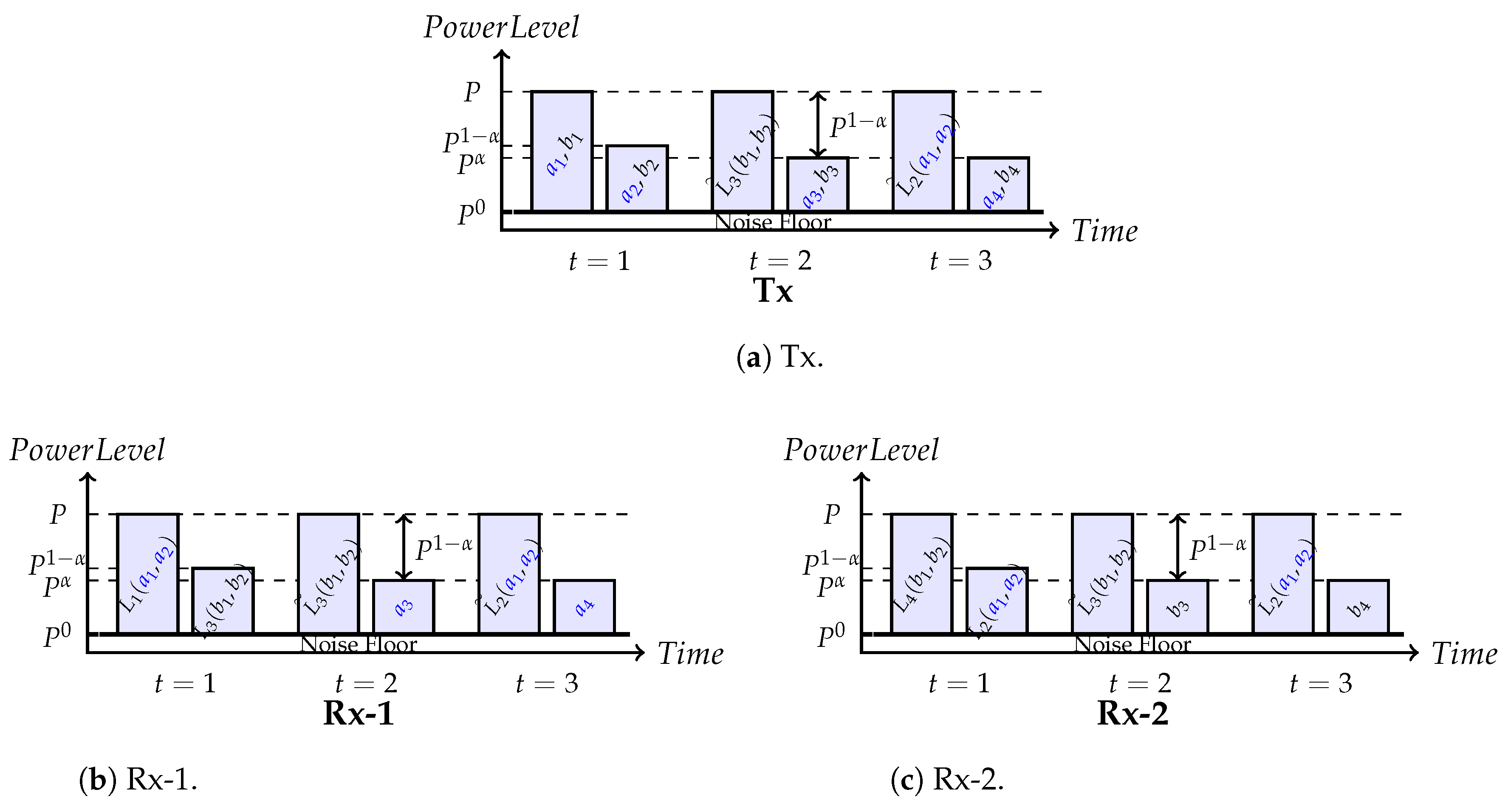
Figure 6.
DoF as a function of for various schemes. The transmitter possesses imperfect instantaneous and delayed CSIT. The estimation error of instantaneous CSIT scales with . Thus, with increasing , the accuracy of instantaneous CSIT improves. Hereby, refers to the state where the instantaneous CSIT accuracy is quasi-perfect in DoF sense, and is when instantaneous CSIT becomes obsolete.
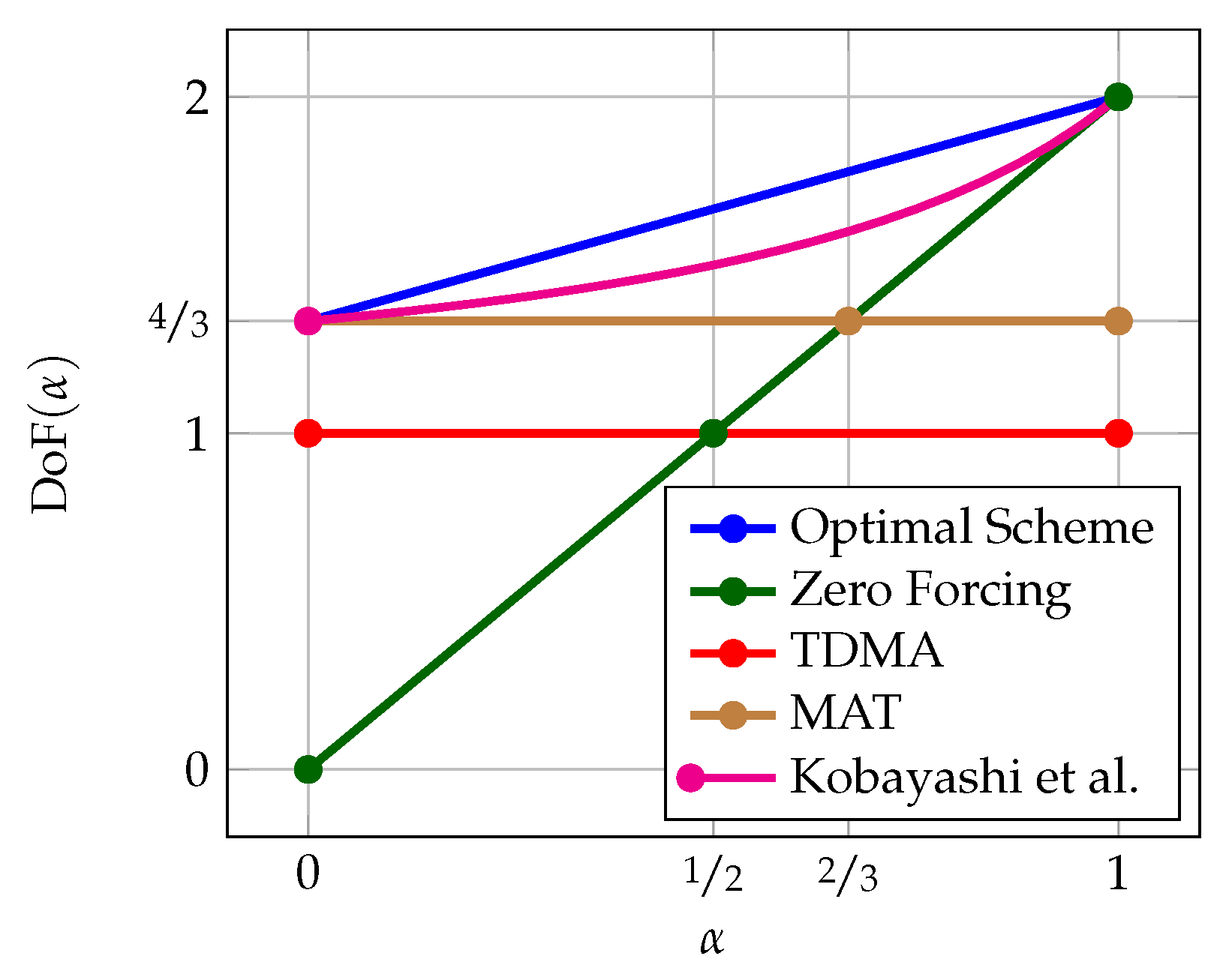
Figure 7.
The figure shows the MISO BC for channels with distinct strengths and that either stay constant (e.g., in (a) and ) or vary in time (b). Furthermore, at any time instant t, the CSIT feedback from Rx-1 and Rx-2 may change and provide the transmitter with distinct CSI states and , respectively. Hereby, P, D and N are perfect, delayed and no CSIT. In the left figure (a), on the one hand, the CSIT state is depicted, whereas the right figure (b), on the other hand, shows the timely static state .
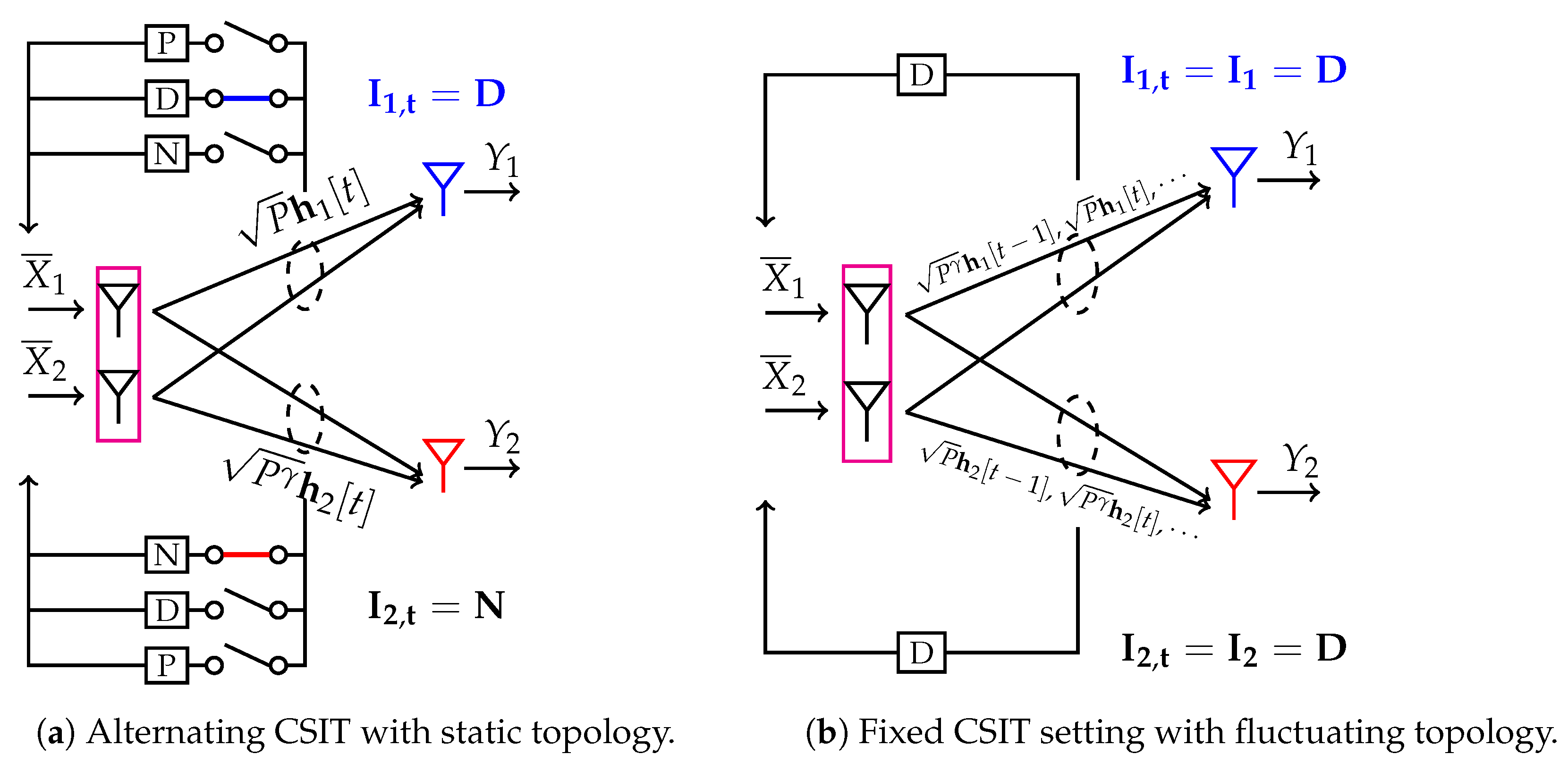
Figure 8.
Plot of upper and lower bounds on the GDoF as a function of for example (a,b). The upper bound is obtained from [62]. We observe that upper and lower bounds only coincide for and in example (a). In example (b), however, we have matching upper and lower bounds for arbitrary .
Figure 8.
Plot of upper and lower bounds on the GDoF as a function of for example (a,b). The upper bound is obtained from [62]. We observe that upper and lower bounds only coincide for and in example (a). In example (b), however, we have matching upper and lower bounds for arbitrary .

Figure 9.
Relaid-aided X-channel with two single-antenna transmitters and receivers supported by a relay node. Hereby, the transmitters are completely blind, i.e., they completely lack CSI. In (a) the relay has a single antenna and perfect global CSI, whereas in (b) the relay has two antennas and delayed global CSI.

Figure 10.
X-channel under mixed CSIT. In addition, only Tx-3 receives partial output feedback from Rx-1.
Figure 10.
X-channel under mixed CSIT. In addition, only Tx-3 receives partial output feedback from Rx-1.
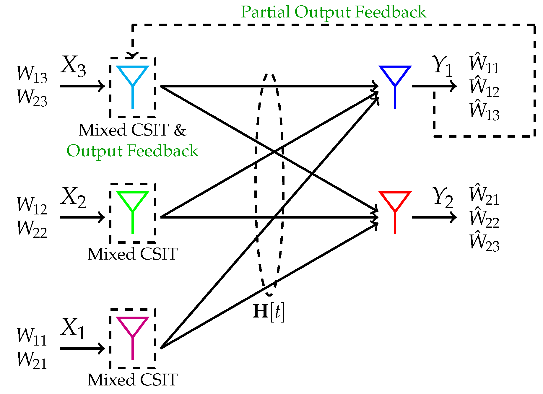
Figure 11.
Outline of the achievability scheme for the X-channel under mixed CSIT. With the exception of phase B, the residual interference that is observed at a particular phase ℓ is transmitted as common information in the consecutive phase in channel uses. Due to this nature, a backward decoding strategy has to be applied.

Figure 12.
The figure plots the achievable DoF as a function of the CSIT quality parameter . For , the CSIT setting reduces to the case of delayed CSI and partial output feedback, while for all transmitters have perfect CSI (in addition to Tx-3’s access to output feedback). An existing upper bound [82] suggests that for the given X-channel, feedback does not increase the DoF in case of perfect CSIT. Thus, a finite quality CSIT of and partial output feedback already attain the optimal .
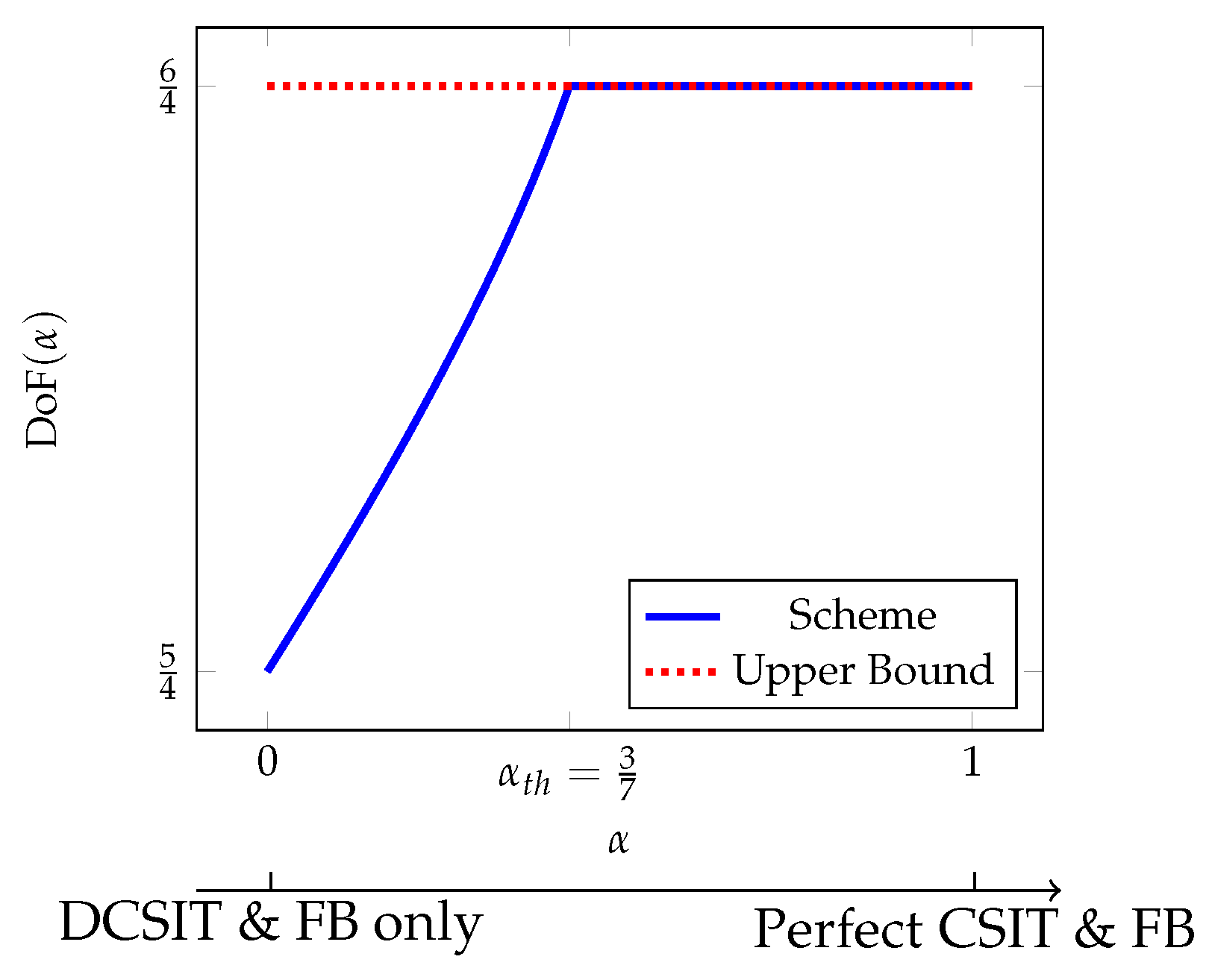
© 2017 by the authors. Licensee MDPI, Basel, Switzerland. This article is an open access article distributed under the terms and conditions of the Creative Commons Attribution (CC BY) license (http://creativecommons.org/licenses/by/4.0/).
Share and Cite
MDPI and ACS Style
Kakar, J.; Sezgin, A. A Survey on Robust Interference Management in Wireless Networks. Entropy 2017, 19, 362. https://doi.org/10.3390/e19070362
AMA Style
Kakar J, Sezgin A. A Survey on Robust Interference Management in Wireless Networks. Entropy. 2017; 19(7):362. https://doi.org/10.3390/e19070362
Chicago/Turabian StyleKakar, Jaber, and Aydin Sezgin. 2017. "A Survey on Robust Interference Management in Wireless Networks" Entropy 19, no. 7: 362. https://doi.org/10.3390/e19070362
Note that from the first issue of 2016, this journal uses article numbers instead of page numbers. See further details here.