A Quantized Kernel Learning Algorithm Using a Minimum Kernel Risk-Sensitive Loss Criterion and Bilateral Gradient Technique


1
School of Computer and Communication Engineering, University of Science and Technology Beijing (USTB), Beijing 100083, China
2
Beijing Key Laboratory of Knowledge Engineering for Materials Science, Beijing 100083, China
3
Department of Computer Science and Information Engineering, National Taipei University of Technology, Taipei 10608, Taiwan
4
Department of Electrical Engineering and Computer Science, Cleveland State University, Cleveland, OH 44115, USA
*
Authors to whom correspondence should be addressed.
Entropy 2017, 19(7), 365; https://doi.org/10.3390/e19070365
Submission received: 19 June 2017
/
Revised: 8 July 2017
/
Accepted: 13 July 2017
/
Published: 20 July 2017
(This article belongs to the Special Issue Entropy in Signal Analysis)
Abstract
:Recently, inspired by correntropy, kernel risk-sensitive loss (KRSL) has emerged as a novel nonlinear similarity measure defined in kernel space, which achieves a better computing performance. After applying the KRSL to adaptive filtering, the corresponding minimum kernel risk-sensitive loss (MKRSL) algorithm has been developed accordingly. However, MKRSL as a traditional kernel adaptive filter (KAF) method, generates a growing radial basis functional (RBF) network. In response to that limitation, through the use of online vector quantization (VQ) technique, this article proposes a novel KAF algorithm, named quantized MKRSL (QMKRSL) to curb the growth of the RBF network structure. Compared with other quantized methods, e.g., quantized kernel least mean square (QKLMS) and quantized kernel maximum correntropy (QKMC), the efficient performance surface makes QMKRSL converge faster and filter more accurately, while maintaining the robustness to outliers. Moreover, considering that QMKRSL using traditional gradient descent method may fail to make full use of the hidden information between the input and output spaces, we also propose an intensified QMKRSL using a bilateral gradient technique named QMKRSL_BG, in an effort to further improve filtering accuracy. Short-term chaotic time-series prediction experiments are conducted to demonstrate the satisfactory performance of our algorithms.
1. Introduction
Online kernel learning (OKL) has become increasingly popular in machine learning due to the fact that it requires much less memory and a lower computational cost to approximate the desired nonlinearity incrementally [1,2,3,4,5]. As a member of OKL, kernel adaptive filters (KAFs) have attracted much attention because of their advantages, including universal approximation capabilities, reasonable computational complexity, and the fact that they lead to convex optimization problems [6]. Mapping data from an input space into the reproducing kernel Hilbert space (RKHS) through a reproducing kernel [7,8], the nonlinear KAF is obtained in the input space through the linear structure of the RKHS. Recently, the KAF has been widely used in signal processing, such as channel estimation, noise cancellation, and system identification [9,10,11,12,13]. Then, there are some typical nonlinear adaptive filtering algorithms, such as the kernel least mean square (KLMS) algorithm [14], the kernel affine projection algorithm [15], the kernel recursive least square (KRLS) algorithm [16], and many others [17,18,19,20,21,22].
These algorithms mentioned above may fail to achieve desirable performance in non-Gaussian noise environments, owing to the fact that they are usually developed on the basis of the mean square error (MSE) criterion, which is a mere second-order statistic and very sensitive to outliers [23]. In the past few years, information theoretic learning (ITL) has been proven to be very efficient and robust in non-Gaussian signal processing [24,25,26]. Different from the conventional second-order statistical measures such as the MSE, ITL uses the information theory descriptors of divergence and entropy as nonparametric cost functions for the adaptive systems [24]. Through Parzen kernel estimation, ITL can capture higher-order statistics of data and achieves better performance than the MSE, especially in non-Gaussian and nonlinear situations [27]. In consideration of this, ITL also offers an effective and efficient way for robust optimization, which has been a popular methodology in the last decade while addressing some optimization problems in the presence of uncertain input data [28,29,30].
In particular, correntropy is a local similarity measure of ITL, defined as a generalized correlation function in kernel space with an effort to estimate the similarity between two random variables [31,32], while achieving some successful applications, e.g., state estimation, image processing, and noise control [33,34,35]. In addition, the corresponding maximum correntropy criterion (MCC) has been used as a cost function to derive various robust nonlinear adaptive filtering algorithms, such as the kernel maximum correntropy (KMC) algorithm [36] and the kernel recursive maximum correntropy (KRMC) algorithm [27], and they show better performance than those classical second-order schemes, e.g., KLMS and KRLS. However, correntropic loss (C-Loss) is a non-convex function, and may converge slowly, especially when the initial value is far away from the optimal value. Recently, a modified similarity measure called kernel risk-sensitive loss (KRSL) was derived in [37], which can be more “convex” and can achieve faster convergence speed and higher filtering accuracy, while maintaining the robustness to outliers. After applying KRSL to adaptive filtering, a new robust KAF algorithm was accordingly proposed [37]. It is called the minimum kernel risk-sensitive loss (MKRSL) algorithm, which could be superior to some existing methods and is attracting growing attention.
One of the limitations in the KAF is the linearly growing radial basis functional (RBF) network structure with each input sample, which leads to the increase of memory requirement and computational complexity [17]. Hence, many sparsification methods have been developed to curb the growth structure, such as the surprise criterion (SC) [38], novelty criterion (NC) [39], coherence criterion [40], and approximate linear dependency (ALD) criterion [16]. Although these methods can significantly curb the network size, the high computing cost still imposes a very challenging obstacle to their practical applications. Moreover, these methods purely discard the redundant data, which may lead to a reduction in filtering accuracy. Then, the online vector quantization (VQ) method was applied to KAFs, constraining their network size through a simple distance calculation. The quantization method is computationally simple, and the redundant data are used to update the coefficient of the closest center, which leads to the improvement of filtering accuracy.
To limit the network size of the MKRSL algorithm, in this article we propose a novel KAF algorithm, named quantized MKRSL (QMKRSL), using the online VQ method. However, the QMKRSL using traditional gradient descent method may not make full use of hidden information between the input and output spaces, where the difference between those samples in a same quantization region could be ignored [41]. To further improve solution accuracy, we also propose an intensified QMKRSL using a bilateral gradient technique named QMKRSL_BG, which can adjust the coefficient vector of the closest center and the current desired output related to a same quantization region simultaneously when a new input sample is discarded.
The rest of this article is organized as follows. Section 2 provides a brief review of KRSL and MKRSL. Then, the details of the proposed algorithms QMKRSL and QMKRSL_BG are described in Section 3. Finally, short-term chaotic time-series prediction experiments are conducted in Section 4, and the conclusion is summarized in Section 5.
2. Backgrounds
2.1. The Kernel Risk-Sensitive Loss (KRSL) Algorithm
Correntropy measures the similarity of two random variables in the neighborhood of the joint space controlled by the kernel bandwidth [32]. This locality allows the correntropy to be robust to outliers. Based on the MCC, many robust learning algorithms have been developed [42,43]. Among them, the kernel bandwidth is a key parameter in the MCC. Generally, a smaller kernel bandwidth makes the algorithm more robust to outliers, but results in slow convergence speed and poor accuracy. On the other hand, when kernel bandwidth becomes larger, the robustness will be significantly reduced when outliers appear. To achieve better performance, a new similarity measure, i.e., KRSL, was proposed in [37], which can be more “convex” and thus can achieve faster convergence rate and higher filtering accuracy while maintaining the robustness to outliers.
Given two random variables X and Y with joint distribution function , the KRSL is defined as follows:
where represents the risk-sensitive parameter, is a shift-invariant Mercer kernel, and represents the kernel bandwidth that controls the range in which similarity is estimated. In addition, denotes the expectation operator. Typically, the kernel used in KRSL is the Gaussian kernel, given by:
where . In practice, since the joint distribution of X and Y is usually unknown, we only use a finite number of data samples to approximate the expectation:
Then, the approximation of KRSL can also be considered as a distance between the vectors and .
In contrast to correntropy, the performance surface of the KRSL can be more “convex”. The areas around the optimal solution are relatively flat to reduce the misadjustments, and the areas away from the optimal solution become steep to speed up the convergence. Moreover, the areas further away from the optimum gradually become entirely flat to avoid the big fluctuations caused by large outliers. Hence, KRSL can provide a more efficient solution that can achieve both a faster convergence rate and higher filtering accuracy while maintaining the robustness to outliers.
Remark 1.
Actually, both C-Loss and KRSL are non-convex functions. However, compared with C-Loss, the performance surface of KRSL can make the gradient-based search algorithms approach the optimal solution more effectively and accurately. Hence, in this article we call KRSL more “convex” than C-Loss.
2.2. Minimum Kernel Risk-Sensitive Loss (MKRSL) Algorithm
Just like MSE and MCC, KRSL function can also be used as a cost function in adaptive filters. In so doing, the goal is to minimize the KRSL function between the desired signal and the filter output . This optimization principle is called the MKRSL criterion, given by:
where represents the input vector, is the prediction error at time i, N is the number of samples, is a Mercer kernel with kernel bandwidth which is used to calculate the KRSL, and is the estimated value of the filter weight vector.
In accordance with the stochastic gradient descent method, the instantaneous cost function of the MKRSL algorithm at time i is defined as:
Then the process of updating the weight can be easily derived as:
where denotes the estimated weight vector at iteration i, is a learning update parameter, and is the step-size parameter.
The performance of linear adaptive filters will degrade dramatically when the mapping between input and desired output d is nonlinear. Therefore, the input is transformed into a high-dimensional feature space as through the kernel-induced mapping (7):
where is the input domain and the dimensionality of is infinite while using Gaussian kernel.
For simplicity, we denote . Then, we can obtain the weight update form for the MKRSL algorithm:
The sequential learning rule for the MKRSL algorithm is shown as:
where is the estimate of the nonlinear mappings between inputs and outputs at iteration i, is another kernel (Gaussian) with the kernel bandwidth . Here, is used to calculate the inner product in the RKHS via the following kernel trick:
Through iterations, the system output to a new input can be solely expressed as:
where is the coefficient of center .
For any , the weight update will approach zero when the error tends to infinity, which means that the MKRSL algorithm will be robust to large outliers. The details of the MKRSL algorithm are summarized in Algorithm 1. Here, denotes the coefficient vector at iteration i, and . Additionally, denotes the center set at iteration i.
| Algorithm 1 The minimum kernel risk-sensitive loss (MKRSL) algorithm. |
| Initialization: |
| Choose parameters , , and . |
| , . |
| Computation: |
| while is available do |
| (1) ; |
| (2) ; |
| (3) ; |
| (4) ; |
| (5) . |
| end while |
3. The Proposed Algorithm
3.1. The Quantized MKRSL (QMKRSL) Algorithm
As mentioned above, the MKRSL will generate an RBF network that grows linearly with input. This growing structure results in the significant increase of computing costs and memory requirement, especially in the case of continuous adaptation [17]. The online VQ method has been successfully applied to KAFs for containing their linearly growing RBF network. Here, we incorporate the online VQ method into the MKRSL, thus proposing the QMKRSL algorithm. Here, the QMKRSL algorithm is obtained by quantizing the feature vector in the weight update Equation (8), which can be shown as:
where represents the quantization operator in . However, considering that the dimensionality of the feature space is very high, we usually perform the quantization operation in the input space . Therefore, the learning rule for the QMKRSL algorithm can be derived as:
where is a quantization operator in . Now, the QMKRSL algorithm has been obtained, and the details are described in Algorithm 2. Here, is the quantization size, and denotes the center set at iteration i.
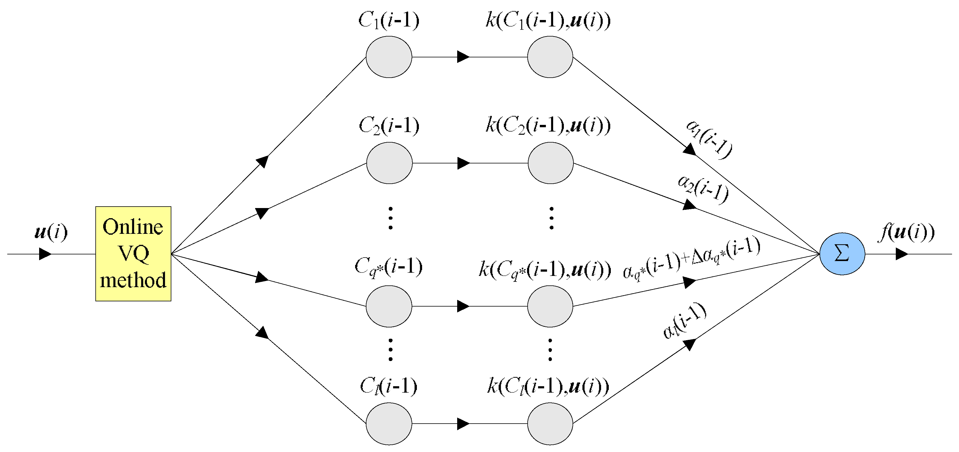
Specifically, in the case that the current sample needs to be quantized, the network topology of QMKRSL is shown in Figure 1. Here, is the closet center of , is the update of the coefficient vector generated by the redundant data , and .
| Algorithm 2 The quantized minimum kernel risk-sensitive loss (QMKRSL) algorithm. |
| Initialization: |
| Choose parameters , , and , . |
| , . |
| Computation: |
| while is available do |
| (1) ; |
| (2) ; |
| (3) ; |
| // compute the distance between and |
| (4) if |
| ; |
| , |
| where ; |
| (5) else |
| ; |
| ; |
| (6) . |
| end while |
As we can see, the quantization approach merely uses the Euclidean distance to determine whether the new input should be added to the dictionary, and updates the coefficient vector of the closest center with the redundant data to improve accuracy. This method is easy to compute and takes full advantage of redundant data rather than discarding them directly, making it possible to avoid the limitations of traditional sparsification methods.
However, it should be noted that the coefficient update process of QMKRSL ignores the difference between the new input sample and its closest center. In addition, the difference between the corresponding desired outputs of the samples in the same quantization region is also neglected. Hence, there is still room for improvement of the QMKRSL algorithm, and the intensified algorithm will be presented in the next subsection.
3.2. The QMKRSL Using Bilateral Gradient Technique (QMKRSL_BG)
In the iterative process, QMKRSL only considers the change of input space, but does not take into account of the difference between the samples in the same quantization region, which may make it unable to make full use of the information hidden in the input and output spaces. Therefore, an efficient way to update the desired output is needed. To further improve the performance, we propose an intensified QMKRSL using bilateral gradient technique, named QMKRSL_BG.
Using the stochastic gradient descent method to minimize the instantaneous cost function (5) in the output space, the current desired output is updated by:
where represents the gradient of the cost function in the desired output direction, is a learning update parameter, and is the step-size parameter used to update the current desired output.
Then, the prediction error and cost function could be updated by:
Similarly, using the stochastic gradient descent method to minimize in the input space, the coefficient update rule of the closest center is derived as:
where is the gradient of the cost function with respect to the coefficient vector, is a learning update parameter, and is the step-size parameter used to update the coefficient of the closest center. In addition, reflects the difference between the input and the its closest center , which can be seen as a weight parameter.
Considering the difference between samples in the same quantization region, the update rules shown in (14)∼(17) could be used when the new sample need to be quantified. For other cases, the update rule for QMKRSL_BG is the same as that of QMKRSL. A specific description of the proposed QMKRSL_BG is summarized in Algorithm 3.
Here, it can easily be found that, through the use of the gradient descent method in output space, QMKRSL_BG employs the prediction error caused by current desired output to update the coefficient vector. Thus, the QMKRSL_BG considers the difference between the desired outputs of samples which are very close in the input space. Moreover, an additive term is introduced in the coefficient update using gradient descent method in input space, which reflects the difference between the current input and the its closest center . Consequently, the QMKRSL_BG can obtain more information from the input and output spaces, so as to achieve better filtering accuracy.
| Algorithm 3 Quantized MKRSL using the bilateral gradient technique (QMKRSL_BG) algorithm. |
| Initialization: |
| Choose parameters , , , and , . |
| , , . |
| Computation: |
| while is available do |
| (1) ; |
| (2) ; |
| (3) ; |
| // compute the distance between and |
| (4) if |
| ; |
| ; |
| ; |
| , |
| where ; |
| (5) else |
| ; |
| ; |
| (6) . |
| end while |
3.3. Complexity Analysis
Here, we will analyze the time complexity of the proposed two algorithms. We can see from the update process that MKRSL shares the computational simplicity of MCC. As shown in (11), the time complexity of MKRSL is , where N represents the number of input samples. Like other quantized methods, e.g., quantized kernel least mean square (QKLMS) and quantized kernel maximum correntropy (QKMC), the key parts of QMKRSL are the calculation for online VQ and updating coefficient vector . Each input sample needs to calculate the Euclidean distance from the dictionary (center set), which means that the complexity of the online VQ method is linearly related to the size of dictionary. According to the above analysis on the output expression of QMKRSL, the time complexity of those two parts of the QMKRSL is , where L represents the network size. Hence, the overall computational complexity of QMKRSL is equal to . Compared with QMKRSL, the proposed QMKRSL_BG only increases the computational effort slightly due to updating the desired output, and it does not affect its practical application.
4. Simulation Results and Discussion
In this section, we conduct simulations related to short-term chaotic time-series prediction, with the purpose of validating the performance of the proposed algorithms QMKRSL and QMKRSL_BG.
4.1. Dataset and Metric
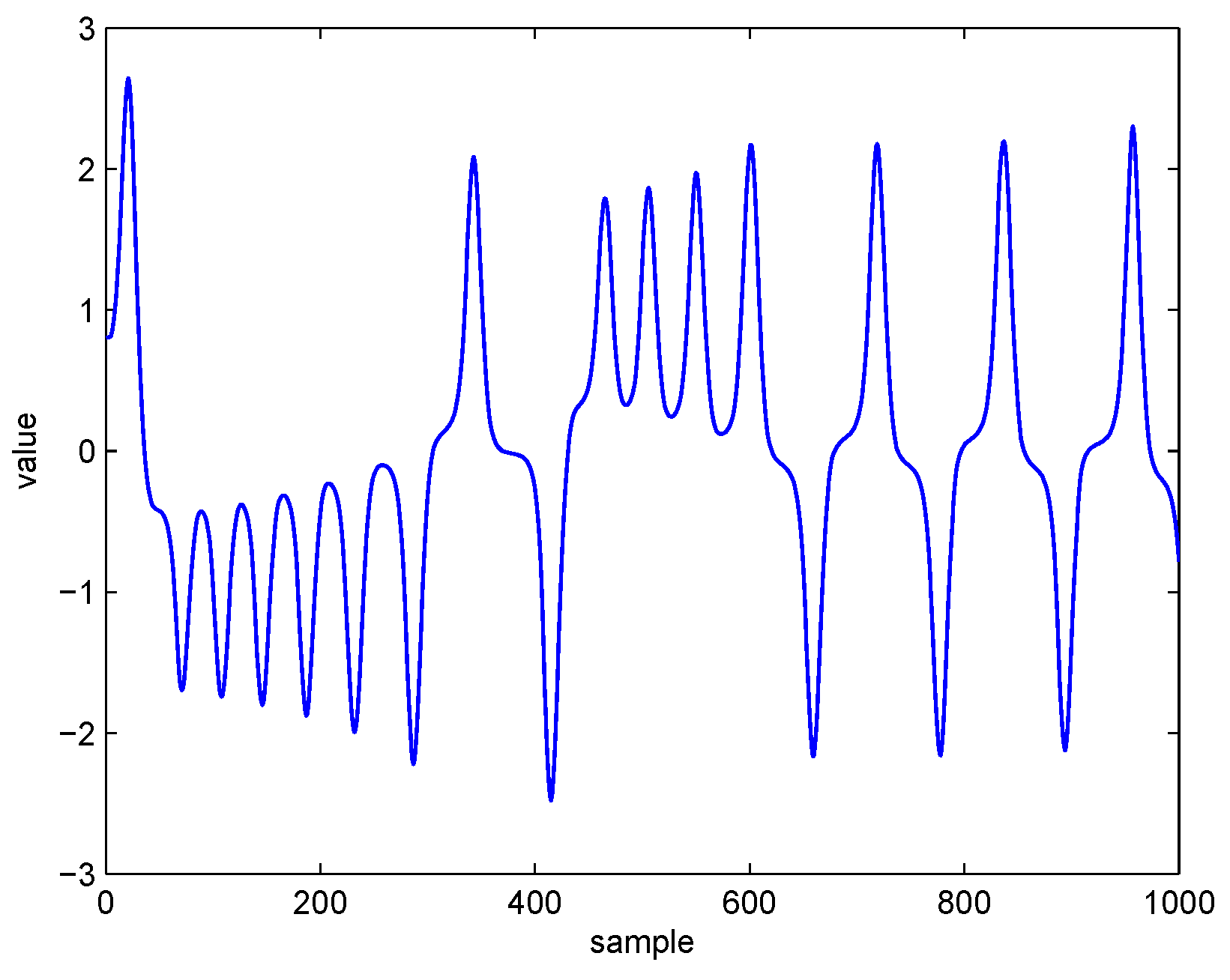
The Lorenz chaotic system is a nonlinear dynamical system with chaotic flow, known for its butterfly shape, which is generated from the following differential equations [44]:
Here the parameters are set as , and . Using this setting, the time-series data are obtained with sampling period 0.01.
We use the first component, i.e., x, to perform the prediction task. The first 1000 samples of the processed Lorenz time-series are shown in Figure 2. In our simulations, we utilize the previous five samples to predict the current point , where and represent the input vector and the corresponding desired output, respectively. Here, we select 4005 continuous samples to generate the training input set () and the corresponding desired output set (), and use the following 1005 samples to generate the testing input set () and the corresponding desired output set ().
In our simulations, the mean square error (MSE) is utilized to evaluate the performance of our proposed algorithms. It is defined as follows:
where N represents the number of predicted values.
In addition to the original MKRSL, the filtering performance is also compared with other quantized methods, including QKLMS and QKMC, under the same simulation condition to demonstrate the superiority of our algorithms. To verify the performance of these algorithms in different noise environments, various noise are adopted in the simulations. They include zero-mean Gaussian noise with variance 0.04, Uniform noise distributed over [−0.3, 0.3], Bernouli noise with variance 0.21, and sine wave noise sin() with uniformly distributed over []. Here, all simulations are performed in a MATLAB computing environment running in an Intel Core i5-3317U, 1.70 GH.
4.2. Simulation Results
The quantization size is a key parameter in quantized KAF algorithms. Hence, we firstly analyze how the performance will be influenced by the quantization size. Generally speaking, the larger the quantization size, the more input vectors need to be quantized to their nearest center, which means that when the quantization size becomes larger, the network size decreases dramatically to a certain degree. While using QMKRSL, the effect of on final network size under different noise environments can be seen in Figure 3. Meanwhile, the final network sizes of QKLMS, QKMC and QMKRSL_BG are equal to that of QMKRSL, because they use the same online VQ method for sparsification, and the quantization parameter has no effect on MKRSL.
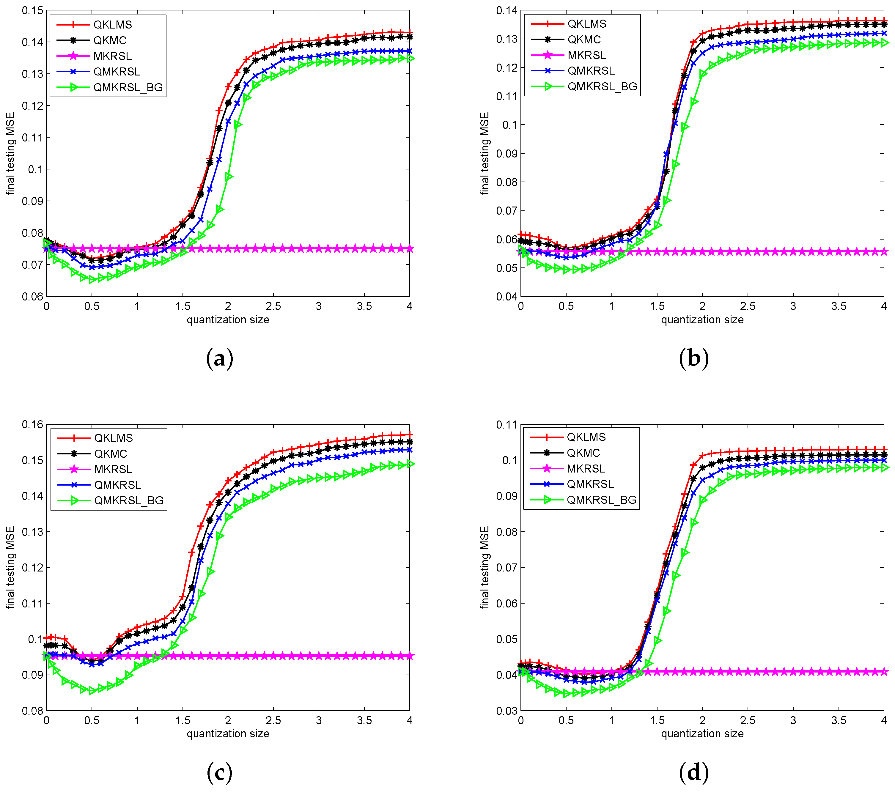
Furthermore, those parameters for all the algorithms under different noise environments are selected in accordance with Table 1. Using these settings, we also show the final testing MSE of these five algorithms under four types of noise environments with different quantization size in Figure 4. Here, the final testing MSE is determined by the average value of the last 200 iterations in the learning curves, and for each iteration, the testing MSE is calculated using 1000 test data. It can be found from Figure 4 that the efficient performance surface makes QMKRSL outperform QKLMS and QKMC in terms of testing MSE. In addition, the bilateral gradient descent method enables QMKRSL_BG to further improve filtering accuracy for all quantization sizes. Due to the fast decrease of network size, the testing MSE will increase significantly when the quantization size increases to a certain degree. Hence, the QMKRSL and QMKRSL_BG are superior to MKRSL when the quantization size is bounded within a certain range. Therefore, we can conclude that the algorithms QMKRSL and QMKRSL_BG can effectively address time-series prediction while constraining the network structure.
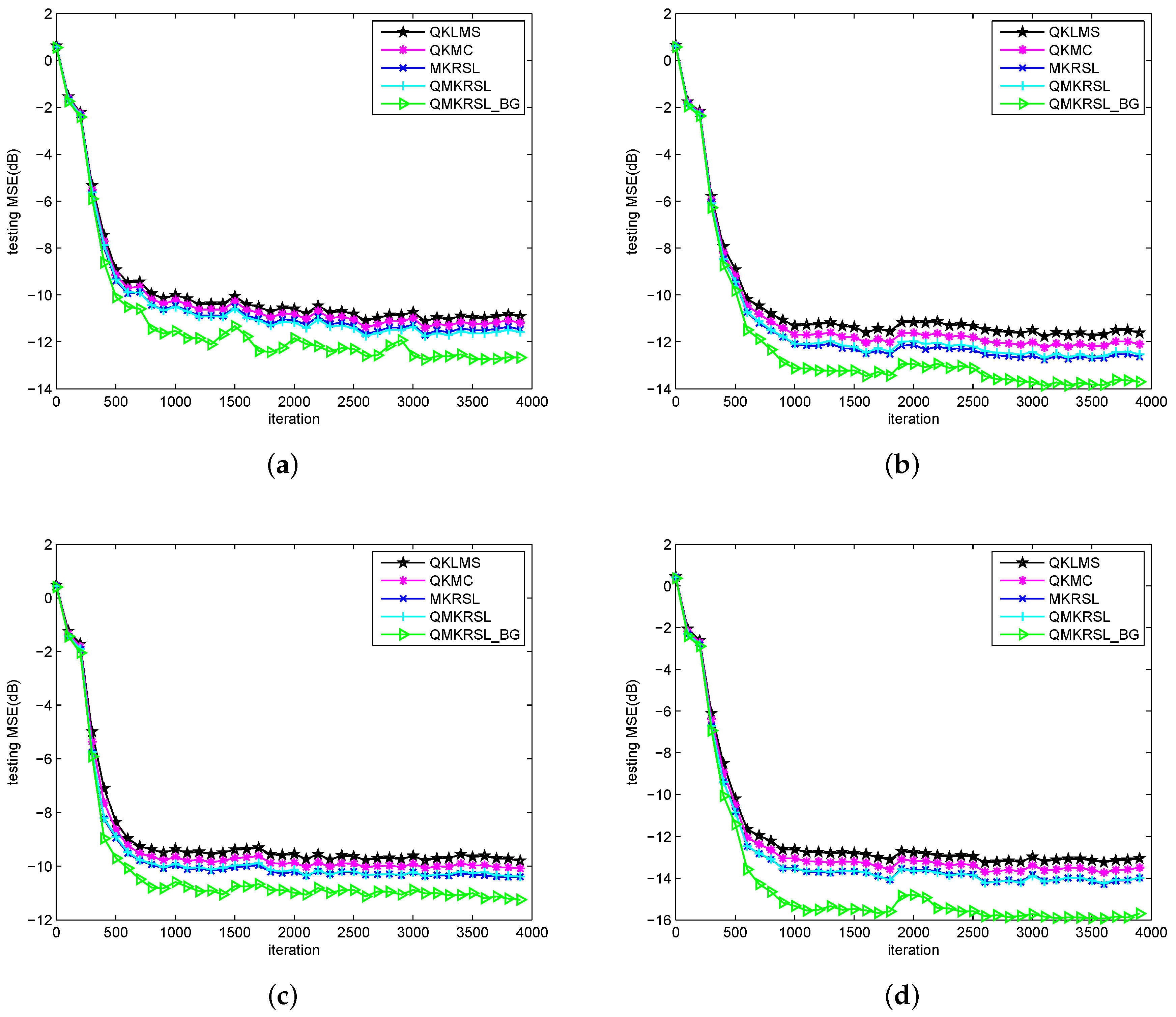
Then, we compare the learning performance of QMKRSL and QMKRSL_BG with that of the original MKRSL, QKLMS, and QKMC, in an effort to demonstrate the superiority of KRSL function and online VQ method. In the simulations below, considering the prediction accuracy and the computational cost simultaneously, we select as 0.2 to make the network size reduce to a modest range, on the basis of the analysis for those results in Figure 3 and Figure 4. Then, the final network sizes for the Gaussian, uniform, Bernouli, and sine wave noise cases are reduced to 2455, 2048, 1373, and 1555, respectively. Therefore, only 2455, 2048, 1373, and 1555 items of training data are chosen as network centers from 4000 input samples for the final filter network.
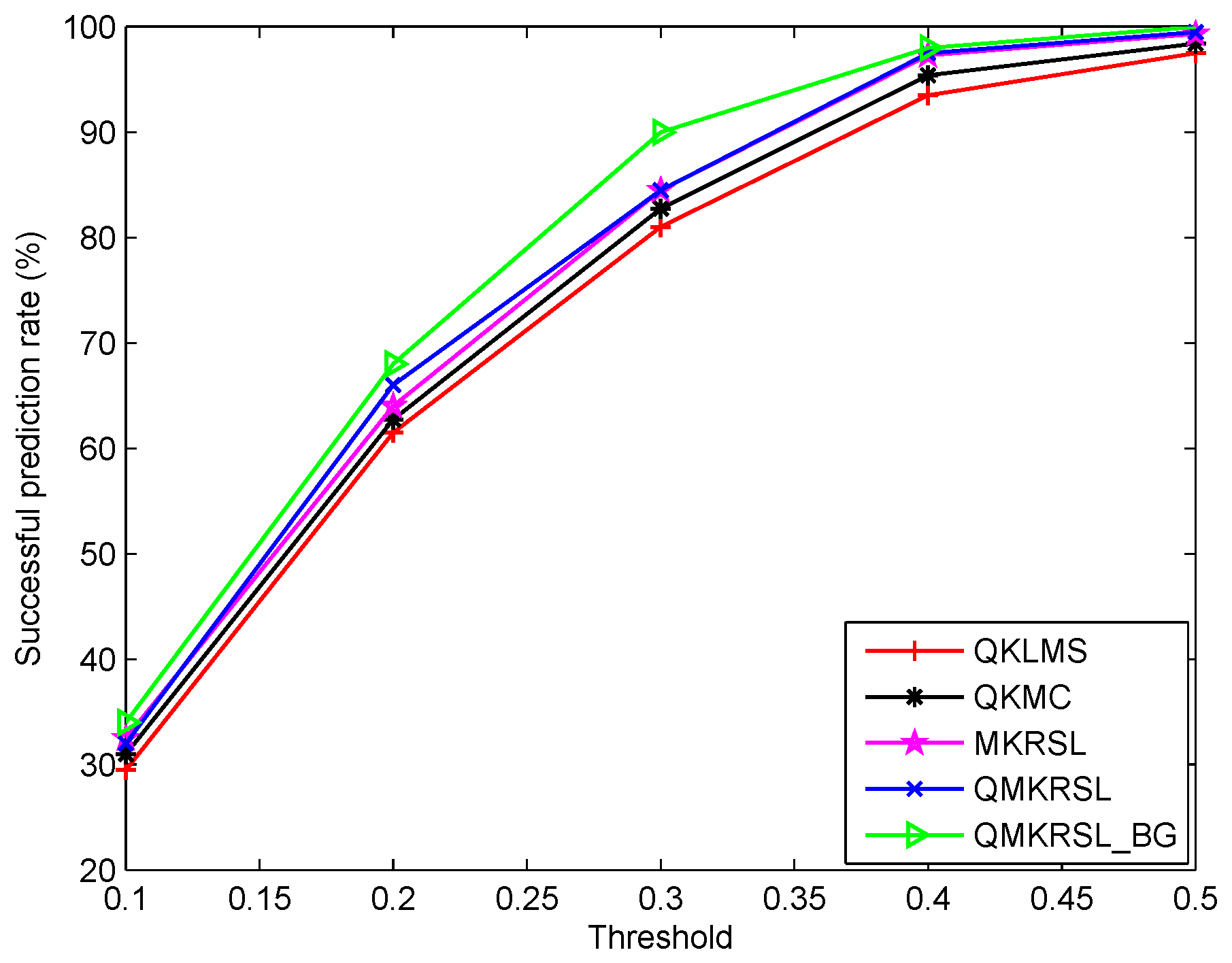
Figure 5 shows the learning curves of these algorithms under different noise environments. It is clear that the testing MSE of the QMKRSL is smaller than that of the QKLMS and the QKMC in all four types of noise environments, and the QMKRSL_BG performs better than all other four algorithms. It indicates that the efficient performance surface of KRSL function can make the QMKRSL outperform the QKMC and QKLMS; the online VQ method using a bilateral gradient technique can obtain more hidden information in the system, and thus the QMKRSL_BG can achieve a higher filtering accuracy than the QMKRSL and other algorithms. Let be the required prediction accuracy. If the prediction error is less than the threshold , the error is within acceptable range and thus the prediction is successful. Otherwise, the prediction fails. With the same noise model used in Figure 5d, the successful prediction rates of these algorithms with changeable threshold are shown in Figure 6. It can be seen that the larger the threshold , the higher the successful rate. Moreover, the successful prediction rate of QMKRSL is similar to that of the MKRSL, and the successful prediction rate of the QMKRSL_BG is higher than other algorithms. This result also verifies that the QMKRSL can maintain the filtering accuracy while effectively limiting the network size, and the QMKRSL_BG can further improve the filtering accuracy.
Hence, in consideration of the final network size and prediction effect simultaneously, the QMKRSL and QMKRSL_BG proposed in this article may be two competitive choices to constrain the network size as well as achieve better prediction performance.
5. Conclusions
On the basis of KRSL criterion, an effective nonlinear KAF algorithm called the MKRSL has been derived to a achieve better filtering performance in non-Gaussian noise environments. To constrain the linearly growing RBF network structure of MKRSL, the quantization technique is incorporated into the original MKRSL, and thus the QMKRSL is proposed in this article. The simulation results of chaotic time-series show that QMKRSL can effectively reduce network size while maintaining simplicity and prediction accuracy. Considering the difference between the samples in a same quantization region, an intensified QMKRSL using the bilateral gradient technique is accordingly developed to further improve the accuracy, and it is named the QMKRSL_BG. In contrast to the traditional gradient descent method, the bilateral gradient descent approach can update the coefficient vector of centers and desired output of samples in the same quantization region simultaneously. This property allows the QMKRSL_BG to get more hidden information from the input and output spaces, and thus achieves higher accuracy. Simulation results have verified the theoretical expectations and demonstrated that the QMKRSL_BG can achieve better filtering performance than some other quantized algorithms. In practical scenarios, computing devices usually have limited computational capacity and physical memory, and are often disturbed by non-Gaussian noises. Therefore, how to effectively constrain the network size as well as achieve higher accuracy in non-Gaussian noise environments is a problem to be solved. In consideration of those facts mentioned above, the proposed algorithms may be the good choices for nonlinear adaptive learning tasks in realistic scenarios.
Due to the smoothness and strict positive-definiteness of Gaussian function, the kernel used in this article defaults to the Gaussian kernel. However, Gaussian kernel is not always the best choice in some cases. Therefore, how to select a better kernel function appropriately is an interesting subject for future study. In addition, as a key parameter in quantized KAF algorithms, the quantization size is determined as a tradeoff between prediction accuracy and computational complexity (network size). Thus, how to select the quantization size appropriately and adaptively is also an important issue to be solved in the future. Moreover, how to achieve good performance when the final network size is fixed in advance is another interesting and important future research topic along this direction.
Acknowledgments
This research is funded by the National Key Technologies R&D Program of China under Grants 2015BAK38B01, the National Natural Science Foundation of China under Grants 61174103 and 61603032, the National Key Research and Development Program of China under Grants 2016YFB0700502, 2016YFB1001404, and 2017YFB0702300, the China Postdoctoral Science Foundation under Grant 2016M590048, the University of Science and Technology Beijing—National Taipei University of Technology Joint Research Program under Grant TW201705, and the Foundation from the National Taipei University of Technology of Taiwan under Grant NTUT-USTB-106-5.
Author Contributions
In this article, Xiong Luo and Weiping Wang provided the original ideas and were responsible for revising the whole article; Jing Deng designed and performed the experiments; Jenq-Haur Wang and Wenbing Zhao analyzed the data. All authors have read and approved the final manuscript.
Conflicts of Interest
The authors declare no conflict of interest.
References
- Kivinen, J.; Smola, A.J.; Williamson, R.C. Online learning with kernels. IEEE Trans. Signal Process. 2004, 52, 2165–2176. [Google Scholar] [CrossRef]
- Gao, W.; Huang, J.G.; Han, J. Online nonlinear adaptive filtering based on multi-kernel learning algorithm. Syst. Eng. Electron. 2014, 36, 1473–1477. [Google Scholar]
- Fan, H.J.; Song, Q.; Yang, X.L.; Xu, Z. Kernel online learning algorithm with state feedbacks. Knowl. Based Syst. 2015, 89, 173–180. [Google Scholar] [CrossRef]
- Lu, J.; Hoi, S.C.H.; Wang, J.L.; Zhao, P.L.; Liu, Z.Y. Large scale online kernel learning. J. Mach. Learn. Res. 2016, 17, 1–43. [Google Scholar]
- Luo, X.; Zhang, D.D.; Yang, L.T.; Liu, J.; Chang, X.H.; Ning, H.S. A kernel machine-based secure data sensing and fusion scheme in wireless sensor networks for the cyber-physical systems. Future Gener. Comput. Syst. 2016, 61, 85–96. [Google Scholar] [CrossRef]
- Liu, W.F.; Príncipe, J.C.; Haykin, S. Kernel Adaptive Filtering; Wiley: Hoboken, NJ, USA, 2011. [Google Scholar]
- Chen, B.D.; Li, L.; Liu, W.F.; Príncipe, J.C. Nonlinear adaptive filtering in kernel spaces. In Springer Handbook of Bio-/Neuroinformatics; Springer: Berlin, Germany, 2014; pp. 715–734. [Google Scholar]
- Burges, C.J.C. A tutorial on support vector machines for pattern recognition. Data Min. Knowl. Discov. 1998, 2, 121–167. [Google Scholar] [CrossRef]
- Li, Y.S.; Jin, Z.; Wang, Y.Y.; Yang, R. A robust sparse adaptive filtering algorithm with a correntropy induced metric constraint for broadband multi-path channel estimation. Entropy 2016, 18, 380. [Google Scholar] [CrossRef]
- Nakajima, Y.; Yukawa, M. Nonlinear channel equalization by multi-kernel adaptive filter. In Proceedings of the IEEE 13th International Workshop on Signal Processing Advances in Wireless Communications, Cesme, Turkey, 17–20 June 2012; pp. 384–388. [Google Scholar]
- Dixit, S.; Nagaria, D. Design and analysis of cascaded LMS adaptive filters for noise cancellation. Circ. Syst. Signal Process. 2017, 36, 742–766. [Google Scholar] [CrossRef]
- Luo, X.; Liu, J.; Zhang, D.D.; Chang, X.H. A large-scale web QoS prediction scheme for the industrial Internet of Things based on a kernel machine learning algorithm. Comput. Networks 2016, 101, 81–89. [Google Scholar] [CrossRef]
- Jiang, S.Y.; Gu, Y.T. Block-sparsity-induced adaptive filter for multi-clustering system identification. IEEE Trans. Signal Process. 2015, 63, 5318–5330. [Google Scholar] [CrossRef]
- Liu, W.F.; Príncipe, P.P.; Principe, J.C. The kernel least mean square algorithm. IEEE Trans. Signal Process. 2008, 56, 543–554. [Google Scholar] [CrossRef]
- Liu, W.F.; Príncipe, J.C. Kernel affine projection algorithms. EURASIP J. Adv. Signal Process. 2007, 2008, 1–12. [Google Scholar]
- Engel, Y.; Mannor, S.; Meir, R. The kernel recursive least-squares algorithm. IEEE Trans. Signal Process. 2004, 52, 2275–2285. [Google Scholar] [CrossRef]
- Chen, B.D.; Zhao, S.L.; Zhu, P.P.; Príncipe, J.C. Quantized kernel least mean square algorithm. IEEE Trans. Neural Netw. Learn. Syst. 2012, 23, 22–32. [Google Scholar] [CrossRef] [PubMed]
- Chen, B.D.; Zhao, S.L.; Zhu, P.P.; Príncipe, J.C. Quantized kernel recursive least squares algorithm. IEEE Trans. Neural Netw. Learn. Syst. 2013, 24, 1484–1491. [Google Scholar] [CrossRef] [PubMed]
- Zhao, S.L.; Chen, B.D.; Príncipe, J.C. Fixed budget quantized kernel least mean square algorithm. Signal Process. 2013, 93, 2759–2770. [Google Scholar] [CrossRef]
- Zhao, S.L.; Chen, B.D.; Cao, Z.; Zhu, P.P.; Príncipe, J.C. Self-organizing kernel adaptive filtering. EURASIP J. Adv. Signal Process. 2016, 2016, 106. [Google Scholar] [CrossRef]
- Luo, X.; Liu, J.; Zhang, D.D.; Wang, W.P.; Zhu, Y.Q. An entropy-based kernel learning scheme toward efficient data prediction in cloud-assisted network environments. Entropy 2016, 18, 274. [Google Scholar] [CrossRef]
- Xu, Y.; Luo, X.; Wang, W.P.; Zhao, W.B. Efficient DV-HOP localization for wireless cyber-physical social sensing system: A correntropy-based neural network learning scheme. Sensors 2017, 17, 135. [Google Scholar] [CrossRef] [PubMed]
- He, R.; Tan, T.; Wang, L. Robust recovery of corrupted low-rank matrix by implicit regularizers. IEEE Trans. Pattern Anal. Mach. Intell. 2014, 36, 770–783. [Google Scholar] [CrossRef] [PubMed]
- Príncipe, J.C. Information Theoretic Learning: Renyi’s Entropy and Kernel Perspectives; Springer: New York, NY, USA, 2010. [Google Scholar]
- Fan, H.J.; Song, Q.; Xu, Z. An information theoretic sparse kernel algorithm for online learning. Expert Syst. Appl. 2014, 41, 4349–4359. [Google Scholar] [CrossRef]
- Erdogmus, D.; Príncipe, J.C. Generalized information potential criterion for adaptive system training. IEEE Trans. Neural Netw. 2002, 13, 1035–1044. [Google Scholar] [CrossRef] [PubMed]
- Wu, Z.Z.; Shi, J.H.; Zhang, X.; Ma, W.T.; Chen, B.D. Kernel recursive maximum correntropy. Signal Process. 2015, 117, 11–16. [Google Scholar] [CrossRef]
- Sra, S.; Nowozin, S.; Wright, S.J. Optimization for Machine Learning; MIT Press: Cambridge, MA, USA, 2011. [Google Scholar]
- Bertsimas, D.; Sim, M. The price of robustness. Oper. Res. 2004, 52, 35–53. [Google Scholar] [CrossRef]
- Büsing, C.; D’Andreagiovanni, F. New results about multi-band uncertainty in robust optimization. Lect. Notes Comput. Sci. 2012, 7276, 63–74. [Google Scholar]
- Santamaria, I.; Pokharel, P.P.; Príncipe, J.C. Generalized correlation function: Definition, properties, and application to blind equalization. IEEE Trans. Signal Process. 2006, 54, 2187–2197. [Google Scholar] [CrossRef]
- Liu, W.F.; Pokharel, P.P.; Príncipe, J.C. Correntropy: Properties and applications in non-Gaussian signal processing. IEEE Trans. Signal Process. 2007, 55, 5286–5298. [Google Scholar] [CrossRef]
- Liu, X.; Qu, H.; Zhao, J.H.; Yue, P.C.; Wang, M. Maximum correntropy unscented kalman filter for spacecraft relative state estimation. Sensors 2016, 16, 1530. [Google Scholar] [CrossRef] [PubMed]
- Zhou, S.P.; Wang, J.J.; Zhang, M.M.; Cai, Q.; Gong, Y.H. Correntropy-based level set method for medical image segmentation and bias correction. Neurocomputing 2017, 234, 216–229. [Google Scholar] [CrossRef]
- Lu, L.; Zhao, H.Q. Active impulsive noise control using maximum correntropy with adaptive kernel size. Mech. Syst. Signal Process. 2017, 87, 180–191. [Google Scholar] [CrossRef]
- Zhao, S.L.; Chen, B.D.; Príncipe, J.C. Kernel adaptive filtering with maximum correntropy criterion. In Proceedings of the International Joint Conference on Neural Network, San Jose, CA, USA, 31 July–5 August 2011; pp. 2012–2017. [Google Scholar]
- Chen, B.D.; Xing, L.; Xu, B.; Zhao, H.Q.; Zheng, N.N.; Príncipe, J.C. Kernel risk-sensitive loss: Definition, properties and application to robust adaptive filtering. IEEE Trans. Signal Process. 2017, 65, 2888–2901. [Google Scholar] [CrossRef]
- Liu, W.F.; Park, I.; Príncipe, J.C. An information theoretic approach of designing sparse kernel adaptive filters. IEEE Trans. Neural Netw. 2009, 20, 1950–1961. [Google Scholar] [CrossRef] [PubMed]
- Platt, J. A resource-allocating network for function interpolation. Neural Comput. 1991, 3, 213–225. [Google Scholar] [CrossRef]
- Richard, C.; Bermudez, J.C.M.; Honeine, P. Online prediction of time series data with kernels. IEEE Trans. Signal Process. 2009, 57, 1058–1067. [Google Scholar] [CrossRef]
- Wang, S.Y.; Zheng, Y.F.; Duan, S.K.; Wang, L.D.; Tan, H.T. Quantized kernel maximum correntropy and its mean square convergence analysis. Dig. Signal Process. 2017, 63, 164–176. [Google Scholar] [CrossRef]
- Liu, Y.; Chen, J.H. Correntropy kernel learning for nonlinear system identification with outliers. Ind. Eng. Chem. Res. 2013, 53, 5248–5260. [Google Scholar] [CrossRef]
- Wu, Z.Z.; Peng, S.Y.; Chen, B.D.; Zhao, H.Q. Robust Hammerstein adaptive filtering under maximum correntropy criterion. Entropy 2015, 17, 7149–7166. [Google Scholar] [CrossRef]
- Liu, W.F.; Park, I.; Wang, Y.W.; Príncipe, J.C. Extended kernel recursive least squares algorithm. IEEE Trans. Signal Process. 2009, 57, 3801–3814. [Google Scholar]
Figure 1.
Network topology for quantization operation in the i-th iteration computation of the quantized minimum kernel risk-sensitive loss (QMKRSL). VQ: vector quantization.
Figure 1.
Network topology for quantization operation in the i-th iteration computation of the quantized minimum kernel risk-sensitive loss (QMKRSL). VQ: vector quantization.

Figure 2.
The portion of the processed Lorenz time-series.

Figure 3.
The effect of the quantization size on final network size under different noise environments using QMKRSL.
Figure 3.
The effect of the quantization size on final network size under different noise environments using QMKRSL.
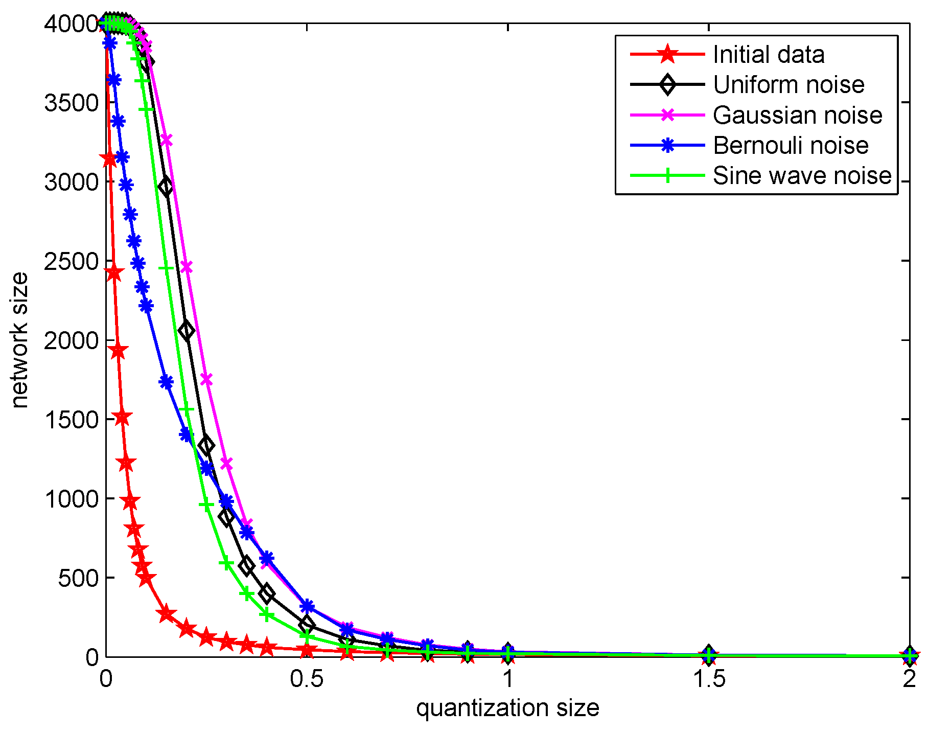
Figure 4.
The effect of the quantization size on final testing mean square error (MSE) under different noise environments: (a) Gaussian; (b) uniform; (c) Bernouli; (d) sine wave.
Figure 4.
The effect of the quantization size on final testing mean square error (MSE) under different noise environments: (a) Gaussian; (b) uniform; (c) Bernouli; (d) sine wave.

Figure 5.
Learning curves in terms of the testing MSE for QKLMS, QKMC, MKRSL, QMKRSL, and QMKRSL_BG under different noise environments: (a) Gaussian; (b) uniform; (c) Bernouli; (d) sine wave.
Figure 5.
Learning curves in terms of the testing MSE for QKLMS, QKMC, MKRSL, QMKRSL, and QMKRSL_BG under different noise environments: (a) Gaussian; (b) uniform; (c) Bernouli; (d) sine wave.

Figure 6.
The successful prediction rates of QKLMS, QKMC, MKRSL, QMKRSL, and QMKRSL_BG with different threshold under sine wave noise environment.
Figure 6.
The successful prediction rates of QKLMS, QKMC, MKRSL, QMKRSL, and QMKRSL_BG with different threshold under sine wave noise environment.


Table 1.
Parameter settings for different algorithms under different noise environments. MKRSL: minimum kernel risk-sensitive loss; QKMC: quantized kernel maximum correntropy; QKLMS: quantized kernel least mean square; QMKRSL_BG: quantized MKRSL using the bilateral gradient technique.
Table 1.
Parameter settings for different algorithms under different noise environments. MKRSL: minimum kernel risk-sensitive loss; QKMC: quantized kernel maximum correntropy; QKLMS: quantized kernel least mean square; QMKRSL_BG: quantized MKRSL using the bilateral gradient technique.
| Noise | QKLMS | QKMC | MKRSL | QMKRSL | QMKRSL_BG |
|---|---|---|---|---|---|
| Gaussian | |||||
| Uniform | |||||
| Bernouli | |||||
| Sine wave |
© 2017 by the authors. Licensee MDPI, Basel, Switzerland. This article is an open access article distributed under the terms and conditions of the Creative Commons Attribution (CC BY) license (http://creativecommons.org/licenses/by/4.0/).
Share and Cite
MDPI and ACS Style
Luo, X.; Deng, J.; Wang, W.; Wang, J.-H.; Zhao, W. A Quantized Kernel Learning Algorithm Using a Minimum Kernel Risk-Sensitive Loss Criterion and Bilateral Gradient Technique. Entropy 2017, 19, 365. https://doi.org/10.3390/e19070365
AMA Style
Luo X, Deng J, Wang W, Wang J-H, Zhao W. A Quantized Kernel Learning Algorithm Using a Minimum Kernel Risk-Sensitive Loss Criterion and Bilateral Gradient Technique. Entropy. 2017; 19(7):365. https://doi.org/10.3390/e19070365
Chicago/Turabian StyleLuo, Xiong, Jing Deng, Weiping Wang, Jenq-Haur Wang, and Wenbing Zhao. 2017. "A Quantized Kernel Learning Algorithm Using a Minimum Kernel Risk-Sensitive Loss Criterion and Bilateral Gradient Technique" Entropy 19, no. 7: 365. https://doi.org/10.3390/e19070365
Note that from the first issue of 2016, this journal uses article numbers instead of page numbers. See further details here.