A Novel Numerical Approach for a Nonlinear Fractional Dynamical Model of Interpersonal and Romantic Relationships


1
Department of Mathematics, JECRC University, Jaipur, Rajasthan 303905, India
2
Department of Mathematics, College of Science, King Saud University, Riyadh 11495, Saudi Arabia
3
Department of Mathematics, Faculty of Arts and Sciences, Cankaya University, Eskisehir Yolu 29. Km, Yukarıyurtcu Mahallesi Mimar Sinan Caddesi No: 4, Etimesgut 06790, Turkey
4
Institute of Space Sciences, P.O. Box MG-23, Magurele-Bucharest 76911, Romania
*
Author to whom correspondence should be addressed.
Entropy 2017, 19(7), 375; https://doi.org/10.3390/e19070375
Submission received: 28 May 2017
/
Revised: 4 July 2017
/
Accepted: 19 July 2017
/
Published: 22 July 2017
(This article belongs to the Special Issue Complex Systems and Fractional Dynamics)
Abstract
:In this paper, we propose a new numerical algorithm, namely q-homotopy analysis Sumudu transform method (q-HASTM), to obtain the approximate solution for the nonlinear fractional dynamical model of interpersonal and romantic relationships. The suggested algorithm examines the dynamics of love affairs between couples. The q-HASTM is a creative combination of Sumudu transform technique, q-homotopy analysis method and homotopy polynomials that makes the calculation very easy. To compare the results obtained by using q-HASTM, we solve the same nonlinear problem by Adomian’s decomposition method (ADM). The convergence of the q-HASTM series solution for the model is adapted and controlled by auxiliary parameter and asymptotic parameter n. The numerical results are demonstrated graphically and in tabular form. The result obtained by employing the proposed scheme reveals that the approach is very accurate, effective, flexible, simple to apply and computationally very nice.
1. Introduction
The theory of entropy was originally related with thermodynamics, but in recent years it has also been used in other areas of investigation such as information theory, psychodynamics, thermoeconomics, human relationships and many more. The second law of thermodynamics states that entropy increases with time. It indicates the instability of a system over a period of time if there is nothing to stabilize it. Similarly, in human relationships, we have daily interactions and these relationships also become disordered. We require input to stabilize any relationship, to iron out the wrinkles or differences, so that we don’t possess and store things forever [1,2,3,4]. The study of interpersonal and romantic relations has been gaining popularity during the past ten years. Interpersonal relations occur in many ways, for example marriage, blood relations, close associations, work and clubs. Since 1957, marriage has been investigated scientifically and we can observe some general interpretations which lead to models of marital interactions. The authors were inspired to study why some married couples get a divorce, when some others couples do not divorce. Moreover, among married couples, some are happy, while some are not happy with each other. In today’s scenario around the globe the number of divorce cases in interpersonal and romantic relations for marriage is increasing day to day. A survey in the United States revealed that for a 40 year duration the chances a first marriage will end in divorce are approximately 50 to 67 percent. For the case of a second marriage for the same duration the chance it will end in divorce is 10 percent higher than for a first marriage. Worldwide, the United States has the highest number of divorce cases. In these areas, experiments are inconvenient and may be restricted due to ethical considerations. To study the dynamics of interpersonal and romantic relations in marriage mathematical models can play a key role and in recent years, many scientists and researchers have studied dynamical modelling of interpersonal relations [5,6,7,8].
Fractional order models are very important to study natural problems. It is well known that the nature of the trajectory of the fractional order derivatives is non-local, which describes that the fractional order derivative has memory effect features [9,10,11,12,13], and any dynamical or physical system related to fractional order differential operators has a memory effect, meaning that the future states depend on the present as well as the past states [14,15,16,17,18,19]. In view of the great importance of fractional approaches in real world problems we were motivated to study the nonlinear dynamical model of interpersonal and romantic relationships. There are various analytical and numerical techniques to study such problems. In 1992, Liao proposed an analytic technique known as the homotopy analysis method (HAM) [20,21] for managing nonlinear problems. More recently, the authors of [22,23] have suggested an extension of HAM known as q-homotopy analysis method (q-HAM) to discuss nonlinear mathematical models. Standard analytical schemes requisite more computer memory and computational time, thus to overcome these limitations the analytical methods need to be merged with standard integral transform operators to study the nonlinear equations appearing in science and engineering [24,25,26].The key purpose of the present work is to propose a novel numerical approach namely q-homotopy analysis Sumudu transform method (q-HASTM) to solve the nonlinear fractional dynamical model of interpersonal and romantic relations in marriages. The q-HASTM is an elegant amalgamation of the q-HAM, the standard Sumudu transform and the homotopy polynomials. The supremacy of this algorithm is its potential of merging two robust computational approaches for investigating nonlinear fractional differential equations. Moreover, the proposed technique contains an asymptotic parameter n by which we can insure to convergence of a series of problem solutions. The paper is organized as follows: In Section 2, fractional calculus and the Sumudu transform are discussed. In Section 3, a fractional order nonlinear dynamical model of interpersonal and romantic relations in marriages is discussed. In Section 4, the fundamental plan of q-HASTM is proposed. In Section 5, a solution of the fractional model is obtained by employing q-HASTM. In Section 6, the fundamental plan of ADM is discussed. In Section 7, a solution of the mathematical model is obtained by employing ADM. Results and discussion are presented in Section 8. Lastly, in Section 9 the concluding observations are highlighted.
2. Basic Definitions
In this section, we discuss the fundamental definitions of integrals and derivatives of non-integer order and the Sumudu transform.
Definition 1.
The left-sided Riemann-Liouville fractional integral operator of order of a function is given in the following manner [9]:
Definition 2.
If is a function of a variable , then the Caputo fractional derivative of the function is expressed as follows [10]:
for
Now, we present the following relation for the fractional integral in the Riemann-Liouville sense and the fractional derivative operator in the Caputo sense:
Definition 3.
The Sumudu transform is a newly introduced integral operator, which was suggested and developed by Watugala [27].This newly integral transform is expressed and discussed over the set of functions:
as follows:
The pioneer work in connection with the formation of important and basic results of the newly integral transform was conducted by Asiru [28], Belgacem et al. [29,30] and Srivastava et al. [31].
Definition 4.
If is a function of , then the Sumudu transform of the Caputo fractional operator is written as follows [32]:
3. Model Description
We consider a nonlinear dynamical model of interpersonal relations with arbitrary order of the form [8]:
with initial conditions:
Here variable measures the love of individual 1 for his/her partner and measures the love of individual 2 for his/her partner. The positive and negative measurement indicates the feelings of the partners towards each other. In the model, and are real constants. These parameters are described as the oblivion, reaction, and attraction constants. In this model, we suppose that in the absence of partners feelings of each other decay exponentially fast. The romantic style of individuals 1 and 2 specified by the parameters and For example, represents the expanse to which the individual is inspired by one's own feelings. The parameter describes the expanse to which the individual is inspired by the partner and it is expected that individual’s partner are supportive in nature. It measures the inclination to seek or avoid the closeness in the love affair between a couple. Hence, indicates that love measures of when the partner is not present, decay exponentially. The term 1/ai indicates the time required for love to decay.
4. Basic Planof q-HASTM
To discuss the key plan of q-HASTM, we take a nonlinear fractional differential equation of the form:
Here is an unknown function of variable and denotes the fractional operator of order proposed by Caputo, indicates the bounded linear operator in and represents the general nonlinear differential operator in Employing the Sumudu transform on Equation (7), we obtain:
Applying the differentiation aspect of the Sumudu transform, we have the following result:
On simplification, we have:
We define the nonlinear operator by keeping view of Equation (10):
In Equation (11), is the embedding parameter and is known as a real function of and Now we develop the homotopy which is given by Equation (12):
where S indicates the Sumudu transform operator, specify an auxiliary parameter, show an initial approximation of If we set the embedding parameter and then we have:
Thus, when varies from 0 to , then the solution takes place from the initial approximation to the solution Expanding the function in the series form by exerting the Taylor series about we obtain:
where:
If the initial approximation asymptotic parameter and the auxiliary parameter are chosen properly, then Equation (14) converges at , then we get the following result:
which must be one of the solutions of the nonlinear fractional differential Equation (7). By taking into consideration Equation (16), the governing equation can be found from the Equation (12).
We define the vectors as follows:
Now differentiating the equation (12) k-times w.r.t. , then divide by k! and finally setting it yields the following result:
Now employing the inverse of the Sumudu transform operator on Equation (18), we obtain:
where is defined and given as follows:
We define the value of in a new way as:
Using Equation (21) in Equation (19), we get:
The novelty in our proposed approach is that a new correction function (24) is introduced by employing homotopy polynomials. Therefore, from Equation (24), we can calculate the distinct iterates for and the q-HASTM series solution is given as follows:
5. q-HASTM Solution for Nonlinear Fractional Dynamical Model of Interpersonal and Romantic Relationships
In this section, we find the solution of nonlinear fractional dynamical model of interpersonal and romantic relationship written in the following form:
withinitial conditions:
Employing the Sumudu transform operator on Equation (26) and using the initial conditions (27), we get the following results:
Now, we write the nonlinear operator as follows:
and:
thus, we have:
The m-th–order deformation equations are given as follows:
Next, on employing the inverse Sumudu operator, this gives:
Now using the initial approximation and recursive relation (33), we obtain the following iterations of the q-HASTM series solution:
Following the same way the remaining components of the q-HASTM solution can be easilyobtained, hence we obtain the complete solution. Finally, we arrive at the following series solution:
6. Basic Idea of ADM
To demonstrate the ADM solution procedure [34,35], we use a fractional nonlinear differential equation with the initial condition of the form:
here is an unknown function of variable and denotes the fractional operator of order proposed by Caputo, indicates the bounded linear operator in and represents the general nonlinear differential operator in .
Employing the operator on both sides of Equation (36) and making use of result (3), we get:
Further, we decompose the function into sum of an infinite number of components expressed by the decomposition series as follows:
and the nonlinear term can be decomposed as:
where denotes the Adomian polynomials, given as follows:
The components are determined recursively by substituting (38) and (39) into (37) leads to:
This can be written as:
ADM uses the formal recursive relations as:
7. ADM Solution for Nonlinear Fractional Dynamical Model of Interpersonal and Romantic Relationship
To solve the nonlinear fractional dynamical model of interpersonal and romantic relations (26), we apply the operator on both sides of Equation (26) and use result (3) to obtain:
This yields the following recursive relations using Equation (43):
where:
The first few components of the Adomian polynomials are given as follows:
The components of the ADM solution can be simply obtained by making use of the above recursive relation:
and so on. In this way the remaining components of the ADM solution can be determined. Hence, the ADM solution of Equation (26) is given as follows:
which can be recovered from the q-HASTM solution by setting and However, most of the results obtained by using other analytical schemes such as HPM, VIM, DTM, and ADM converge to the corresponding numerical results in a very small region. Instead of these methods, in the case of q-HASTM, we can easily settle and restrict the region of convergence of series solution obtained by q-HASTM by setting appropriate values of and
8. Numerical Simulations
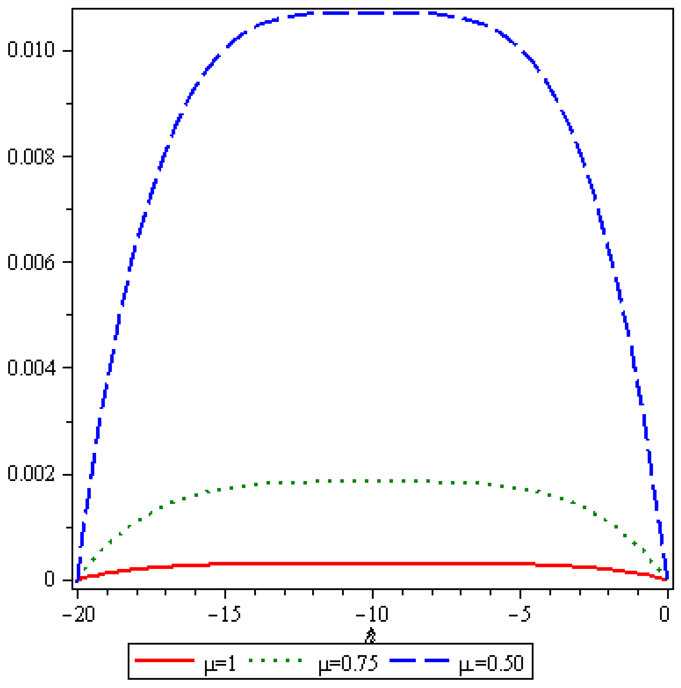
In this section, we perform the numerical simulations for and at the distinct fractional Brownian motions and and also for the standard motion The special solution of fractional dynamical model of the problem is obtained by employing q-HASTM and ADM with different parameters as and The results are shown through Table 1 and Table 2 and Figure 1, Figure 2, Figure 3, Figure 4, Figure 5, Figure 6, Figure 7, Figure 8, Figure 9, Figure 10 and Figure 11. From Table 1 and Table 2, it can be noticed that the values of the approximate solution at distinct grid points obtained by the q-HASTM and ADM are in a very good agreement. Figure 1 and Figure 2 depict the behavior of and for the different values of From Figure 1 we can observe that when we decrease the values of in the fractional dynamic model then the love of individual 1 for his/her partner decreases. From Figure 2 we can observe that when we decrease the value of in the fractional dynamic model then the love of individual 2 for his/her partner decreases. Figure 3, Figure 4 and Figure 5 reveals the behavior of and for the different value of at and From Figure 3, Figure 4 and Figure 5, we see that when we decrease the values of in the fractional dynamic model then romantic relation between the couple decreases. Figure 6, Figure 7 and Figure 8 demonstrate the -curves for at distinct values of and Figure 9, Figure 10 and Figure 11 show the -curves of at distinct values of and The horizontal line segment in -curves shows the range of convergence of q-HASTM solution. From the Figure 6, Figure 7, Figure 8, Figure 9, Figure 10 and Figure 11, it can be noticed that the range of convergence is directly proportional to the value of asymptotic parameter n. Hence, the results obtained by using the proposed technique converge very fast as compared to other existing analytical sachems.
9. Conclusions
In this article, we have proposed a novel numerical method named q-HASTM to solve nonlinear dynamical models of interpersonal and romantic relationships for marriages with a fractional approach and compared the results with ADM. The numerical and graphical results reveal the successfully application of q-HASTM for solving the fractional dynamical model. The results derived with the aid of both the techniques are in an excellent agreement. The displacement shows a new nature for the time fractional derivative compared to the integer order derivative. The convergence of the q-HASTM solution can be adjusted and controlled with the aid of the auxiliary parameter and asymptotic parameter n. The results presented in the form of graphs and -curves indicate that the suggested scheme is very efficient and accurate. Hence, it can be concluded that the proposed approach is highly logical and can be employed to investigate a wide range of nonlinear mathematical models of fractional order appearing in real world problems. Moreover, q-HASTM opens new doors in the fields of mathematical modeling and fractional calculus.
Acknowledgments
The authors extend their appreciation to the International Scientific Partnership Program ISPP at King Saud University for funding this research work through ISPP#63.
Author Contributions
All the authors have worked equally in this manuscript. All the four authors have read and approved the final manuscript.
Conflicts of Interest
The authors declare no conflict of interest.
References
- Machado, J.A.T.; Lopes, A.M. Fractional Jensen–Shannon analysis of the scientific output of researchers in fractional calculus. Entropy 2017, 19, 127. [Google Scholar] [CrossRef]
- Wang, S.; Zhang, Y.; Yang, X.J.; Sun, P.; Dong, Z.C.; Liu, A.; Yuan, T.F. Pathological brain detection by a novel image feature-fractional Fourier entropy. Entropy 2015, 17, 8278–8296. [Google Scholar] [CrossRef]
- Zhan, X.; Ma, J.; Ren, W. Research entropy complexity about the nonlinear dynamic delay game model. Entropy 2017, 19, 22. [Google Scholar] [CrossRef]
- Zhang, Y.; Yang, X.J.; Cattani, C.; Rao, R.V.; Wang, S.; Phillips, P. Tea category identification using a novel fractional Fourier Entropy and Jaya algorithm. Entropy 2016, 18, 77. [Google Scholar] [CrossRef]
- Strogatz, S.H. Nonlinear Dynamics and Chaos: With Applications to Physics, Biology, Chemistry and Engineering; Reading, M.A., Ed.; Addison-Wesley: Boston, MA, USA, 1994. [Google Scholar]
- Rinaldi, S. Love dynamics: The case of linear couples. Appl. Math. Comput. 1998, 95, 181–192. [Google Scholar] [CrossRef]
- Cherif, A.; Barley, K. Stochastic nonlinear dynamics of interpersonal and romantic relationships. Appl. Math. Comput. 2011, 217, 6273–6281. [Google Scholar]
- Ozalp, N.; Koca, I. A fractional order nonlinear dynamical model of interpersonal relationships. Adv. Differ.Equ. 2012, 189, 1–7. [Google Scholar] [CrossRef]
- Podlubny, I. Fractional Differential Equations; Academic Press: New York, NY, USA, 1999. [Google Scholar]
- Caputo, M. Elasticita e Dissipazione; Zani-Chelli: Bologna, Italy, 1969. [Google Scholar]
- Miller, K.S.; Ross, B. An Introduction to the Fractional Calculus and Fractional Differential Equations; Wiley: New York, NY, USA, 1993. [Google Scholar]
- Kilbas, A.A.; Srivastava, H.M.; Trujillo, J.J. Theory and Applications of Fractional Differential Equations; Elsevier: Amsterdam, The Netherlands, 2006. [Google Scholar]
- Carvalho, A.; Pinto, C.M.A. A delay fractional order model for the co-infection of malaria and HIV/AIDS. Int. J. Dynam. Control 2017, 5, 168–186. [Google Scholar] [CrossRef]
- Singh, J.; Kumar, D.; Nieto, J.J. Analysis of an El Nino-Southern Oscillation model with a new fractional derivative. Chaos Soliton Fract. 2017, 99, 109–115. [Google Scholar] [CrossRef]
- Singh, J.; Kumar, D.; Qurashi, M.A.; Baleanu, D. A new fractional model for giving up smoking dynamics. Adv. Differ. Equ. 2017, 2017, 88. [Google Scholar] [CrossRef]
- Kumar, D.; Singh, J.; Baleanu, D. A hybrid computational approach for Klein-Gordon equations on Cantor sets. Nonlinear Dynam. 2017, 87, 511–517. [Google Scholar] [CrossRef]
- Srivastava, H.M.; Kumar, D.; Singh, J. An efficient analytical technique for fractional model of vibration equation. Appl. Math. Model. 2017, 45, 192–204. [Google Scholar] [CrossRef]
- Atangana, A.; Alkahtani, B.T. Analysis of non-homogenous heat model with new trend of derivative with fractional order. Chaos Soliton Fract. 2016, 89, 566–571. [Google Scholar]
- Singh, J.; Kumar, D.; Nieto, J.J. A reliable algorithm for local fractional Tricomi equation arising in fractal transonic flow. Entropy 2016, 18, 206. [Google Scholar] [CrossRef]
- Liao, S.J. Beyond Perturbation: Introduction to Homotopy Analysis Method; Chapman and Hall/CRC: Boca Raton, FL, USA, 2003. [Google Scholar]
- Liao, S.J. On the homotopy analysis method for nonlinear problems. Appl. Math. Comput. 2004, 147, 499–513. [Google Scholar] [CrossRef]
- El-Tawil, M.A.; Huseen, S.N. The q-homotopy analysis method (q- HAM). Int. J. Appl. Math. Mech. 2012, 8, 51–75. [Google Scholar]
- El-Tawil, M.A.; Huseen, S.N. On convergence of the q-homotopy analysis method. Int. J. Contem. Math. Sci. 2013, 8, 481–497. [Google Scholar] [CrossRef]
- Khan, M.; Gondal, M.A.; Hussain, I.; KarimiVanani, S. A new comparative study between homotopy analysis transform method and homotopy perturbation transform method on semi-infinite domain. Math. Comput. Model. 2012, 55, 1143–1150. [Google Scholar] [CrossRef]
- Rathore, S.; Kumar, D.; Singh, J.; Gupta, S. Homotopy analysis sumudu transform method for nonlinear equations. Int. J. Ind. Math. 2012, 4, 301–314. [Google Scholar]
- Zhao, D.; Singh, J.; Kumar, D.; Rathore, S.; Yang, X.J. An efficient computational technique for local fractional heat conduction equations in fractal media. J. Nonlinear Sci. Appl. 2017, 10, 1478–1486. [Google Scholar] [CrossRef]
- Watugala, G.K. Sumudu transform-a new integral transform to solve differential equations and control engineering problems. Math. Eng. Ind. 1998, 6, 319–329. [Google Scholar] [CrossRef]
- Asiru, M.A. Sumudu transform and the solution of integral equation of convolution type. Inter. J. Math. Educ. Sci. Tech. 2001, 32, 906–910. [Google Scholar] [CrossRef]
- Belgacem, F.B.M.; Karaballi, A.A. Sumudu transform fundament properties investigations and applications. Inter. J. Appl. Math. Stoch. Anal. 2006, 2006, 91083. [Google Scholar]
- Belgacem, F.B.M.; Karaballi, A.A.; Kalla, S.L. Analytical investigations of the Sumudu transform and applications to integral production equations. Math. Probl. Eng. 2003, 3, 103–118. [Google Scholar] [CrossRef]
- Srivastava, H.M.; Golmankhaneh, A.K.; Baleanu, D.; Yang, X.J. Local fractional Sumudu transform with application to IVPs on Cantor sets. Abstr. Appl. Anal. 2014, 2014, 620529. [Google Scholar] [CrossRef]
- Chaurasia, V.B.L.; Singh, J. Application of Sumudu transform in Schrödinger equation occurring in quantum mechanics. Appl. Math. Sci. 2010, 4, 2843–2850. [Google Scholar]
- Odibat, Z.; Bataineh, S.A. An adaptation of homotopy analysis method for reliable treatment of strongly nonlinear problems: Construction of homotopy polynomials. Math. Meth. Appl. Sci. 2015, 38, 991–1000. [Google Scholar] [CrossRef]
- Adomian, G. Solving Frontier Problems of Physics: The Decomposition Method; Kluwer Academic Publisher: Boston, MA, USA, 1994. [Google Scholar]
- Odibat, Z.; Momani, S. Numerical methods for nonlinear partial differential equations of fractional order. Appl. Math. Model. 2008, 32, 28–39. [Google Scholar] [CrossRef]
Figure 1.
Behavior of vs.time for distinct values of when and
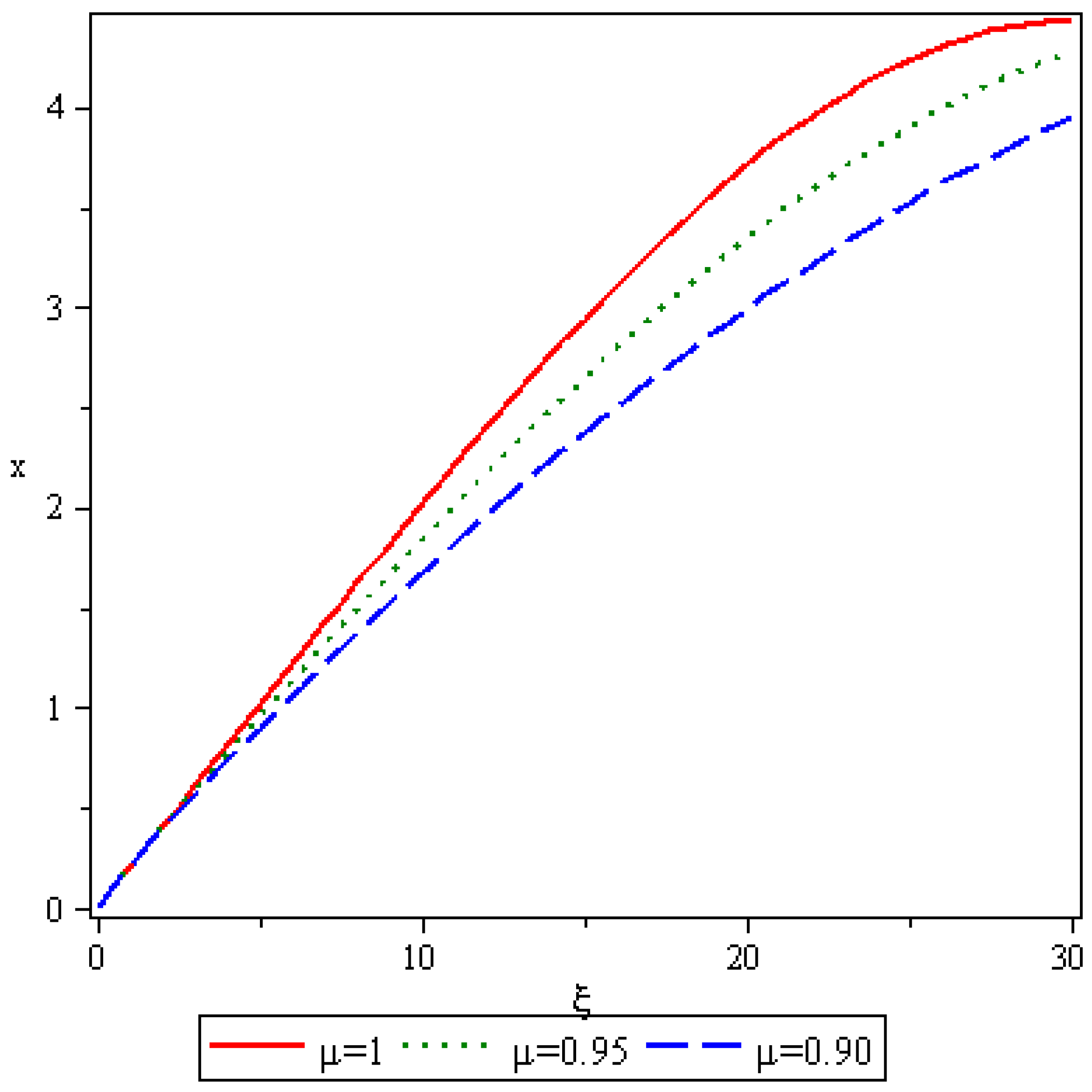
Figure 2.
Nature of vs.time for distinct values of when and
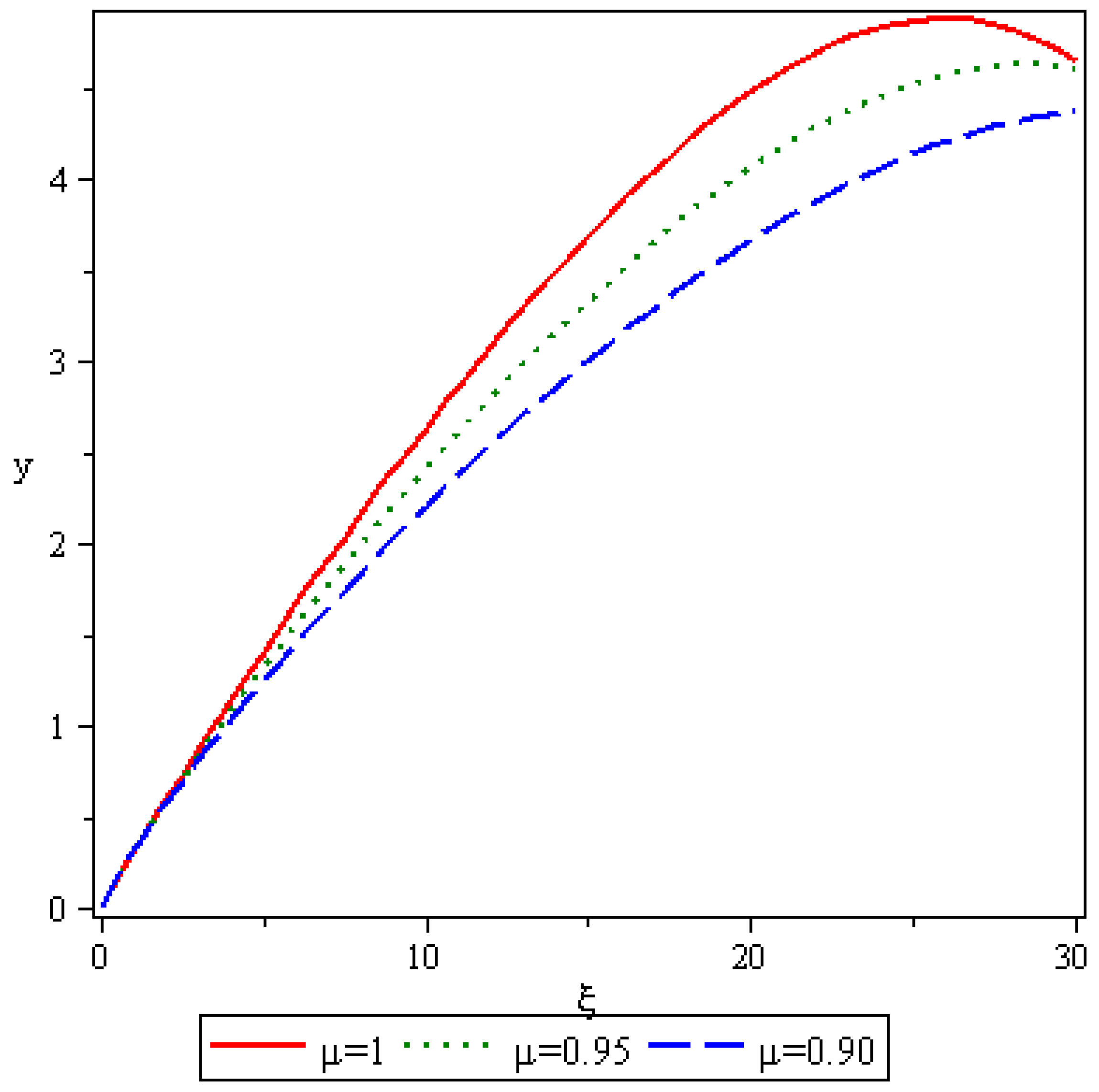
Figure 3.
Behavior of and when and
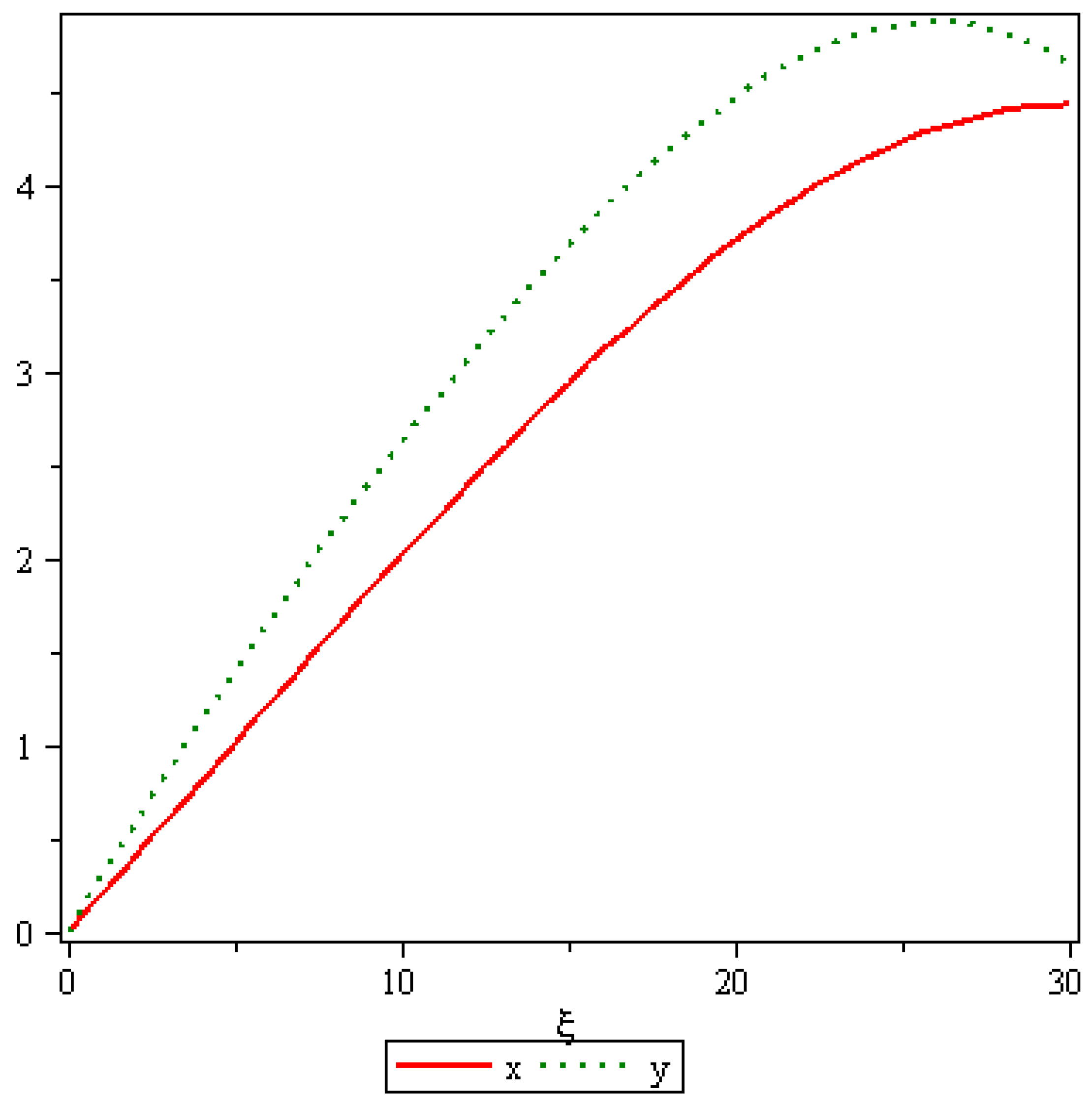
Figure 4.
Characteristic of and when and
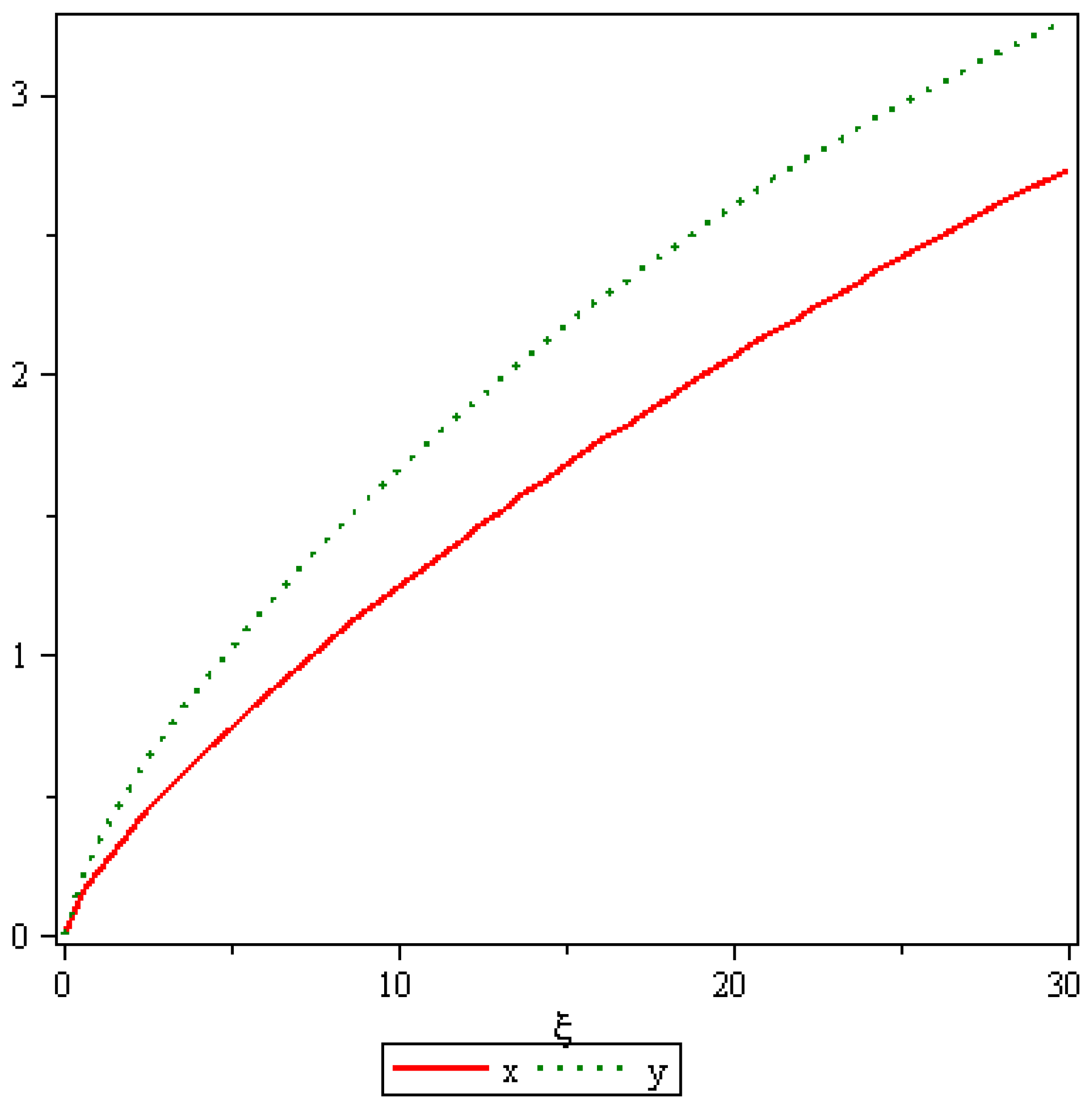
Figure 5.
Response of and when and
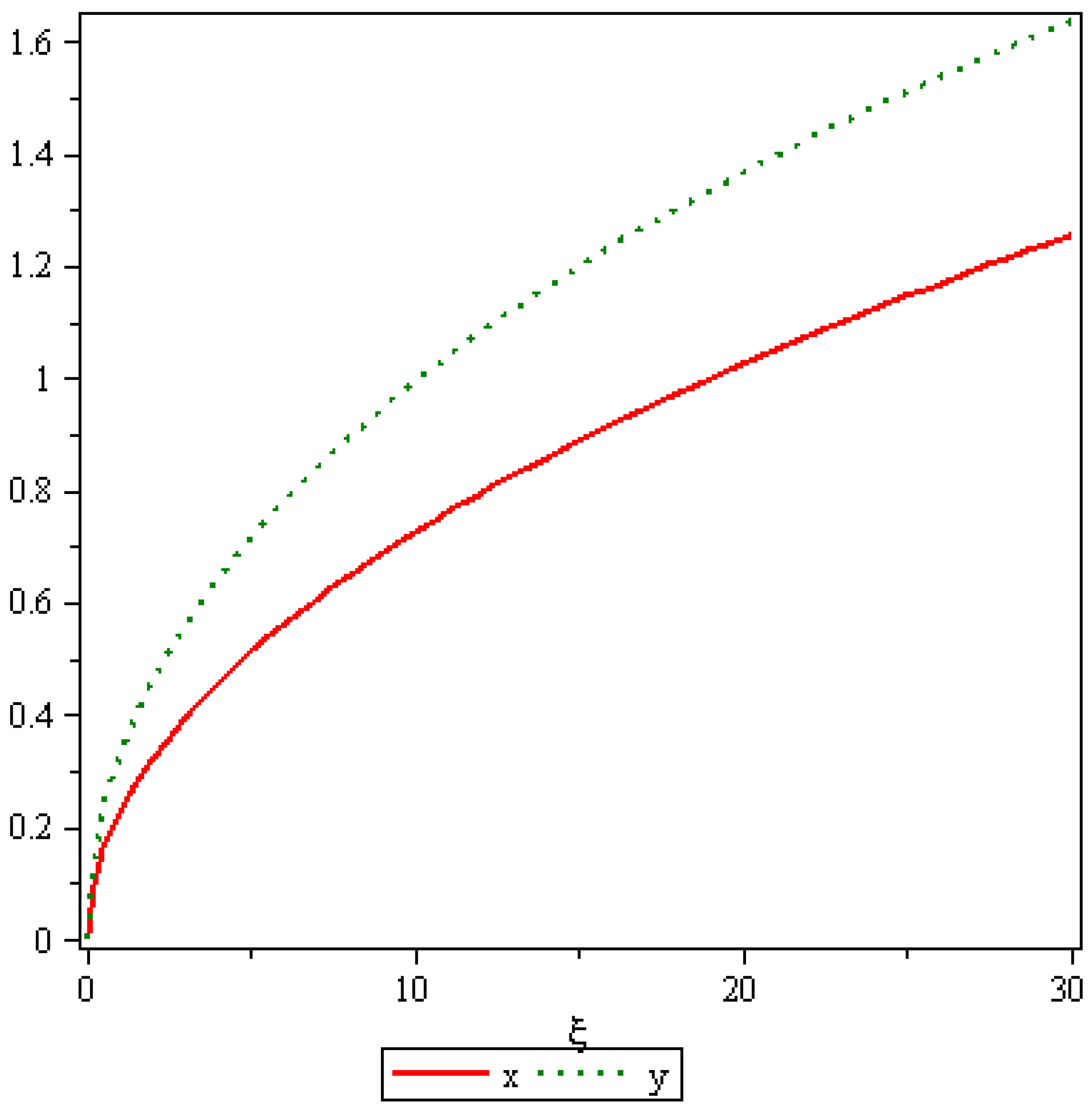
Figure 6.
–curve of for different values of at

Figure 7.
–curve of for different values of at
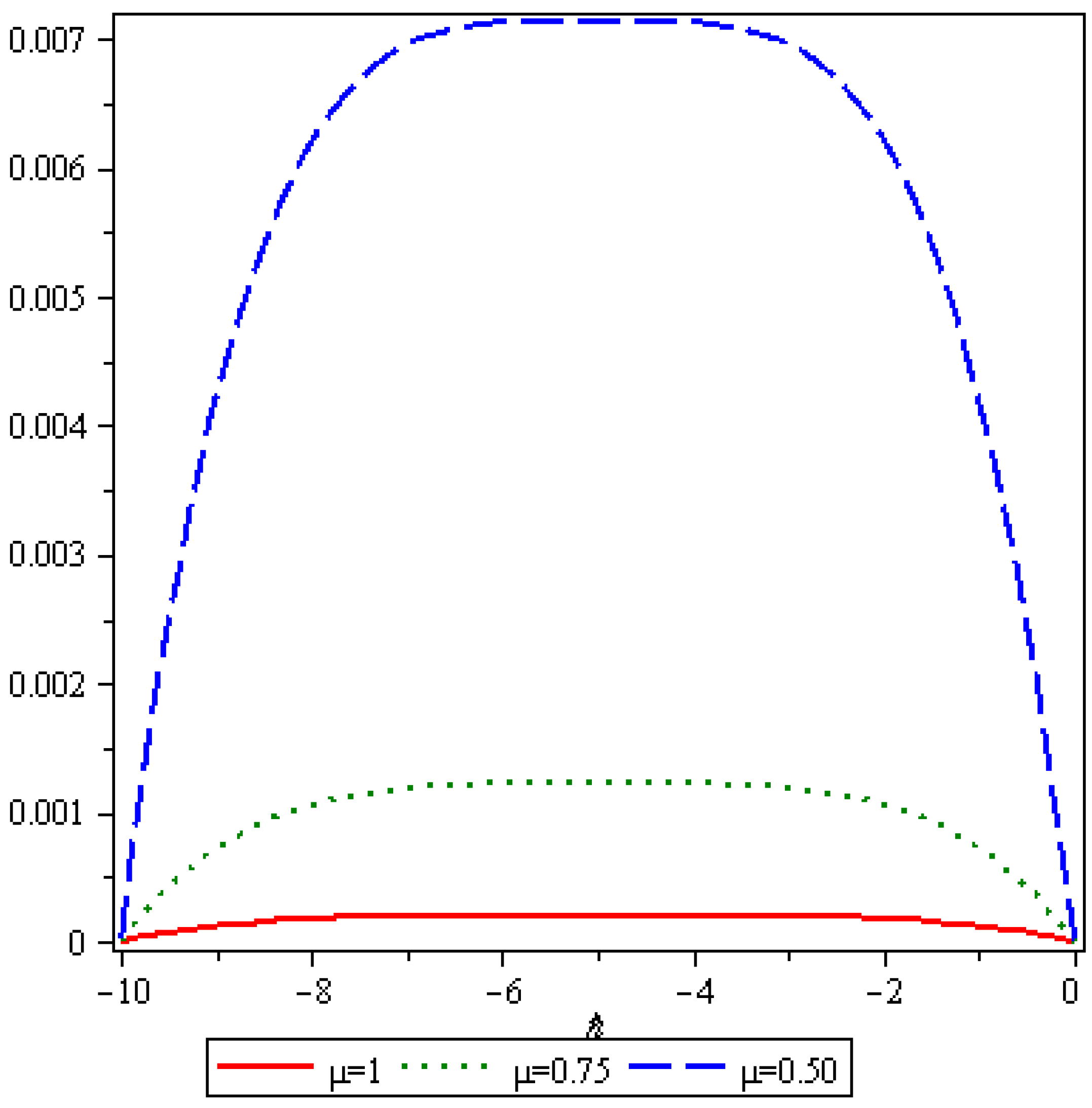
Figure 8.
–curve of for different values of at
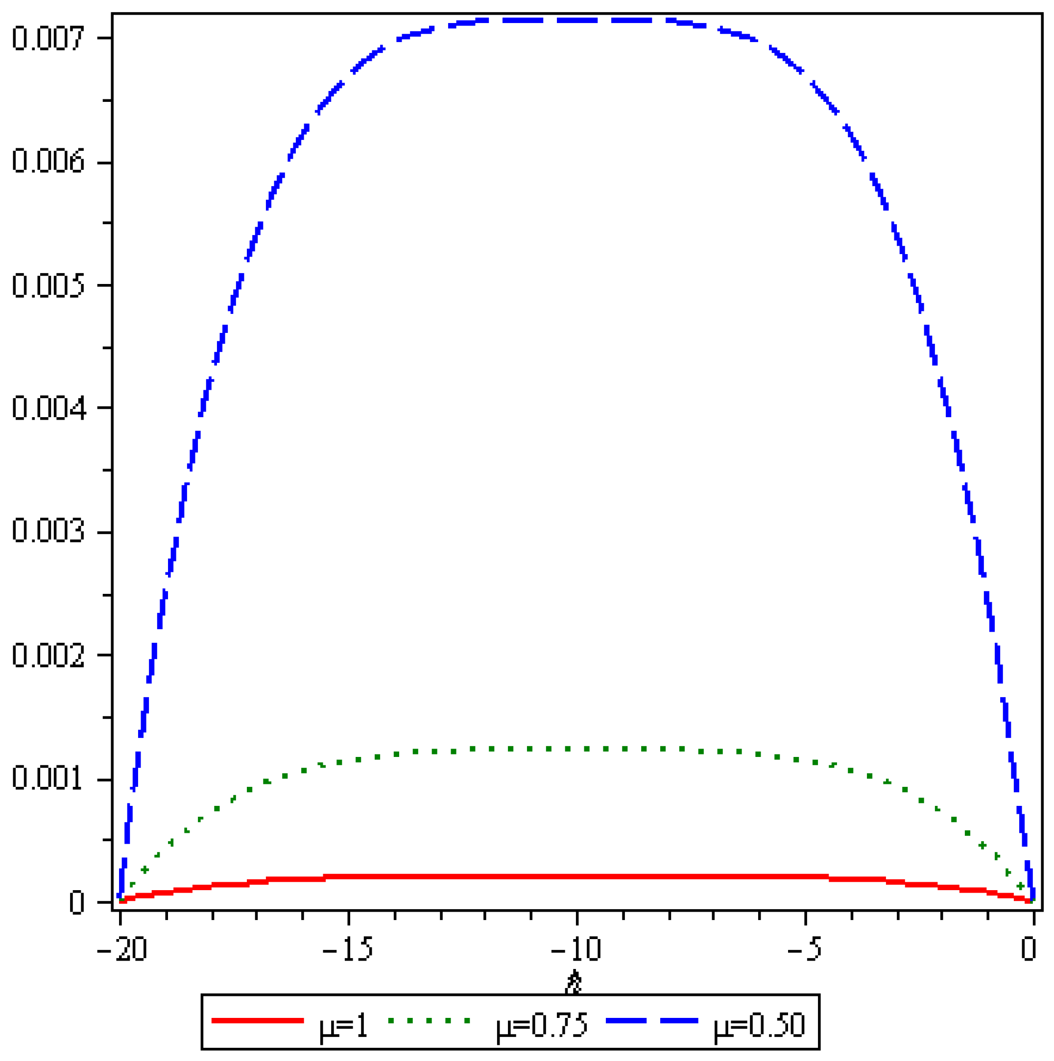
Figure 9.
–curve of for different values of at
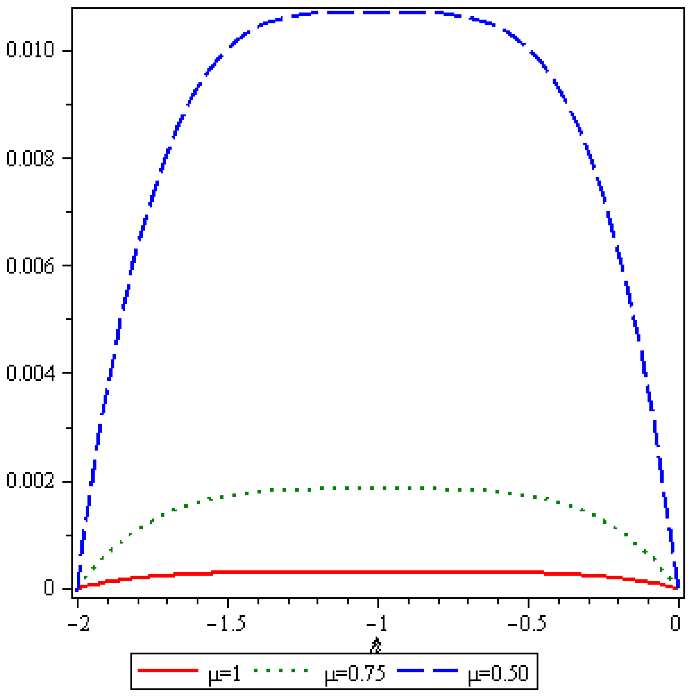
Figure 10.
–curve of for different values of at
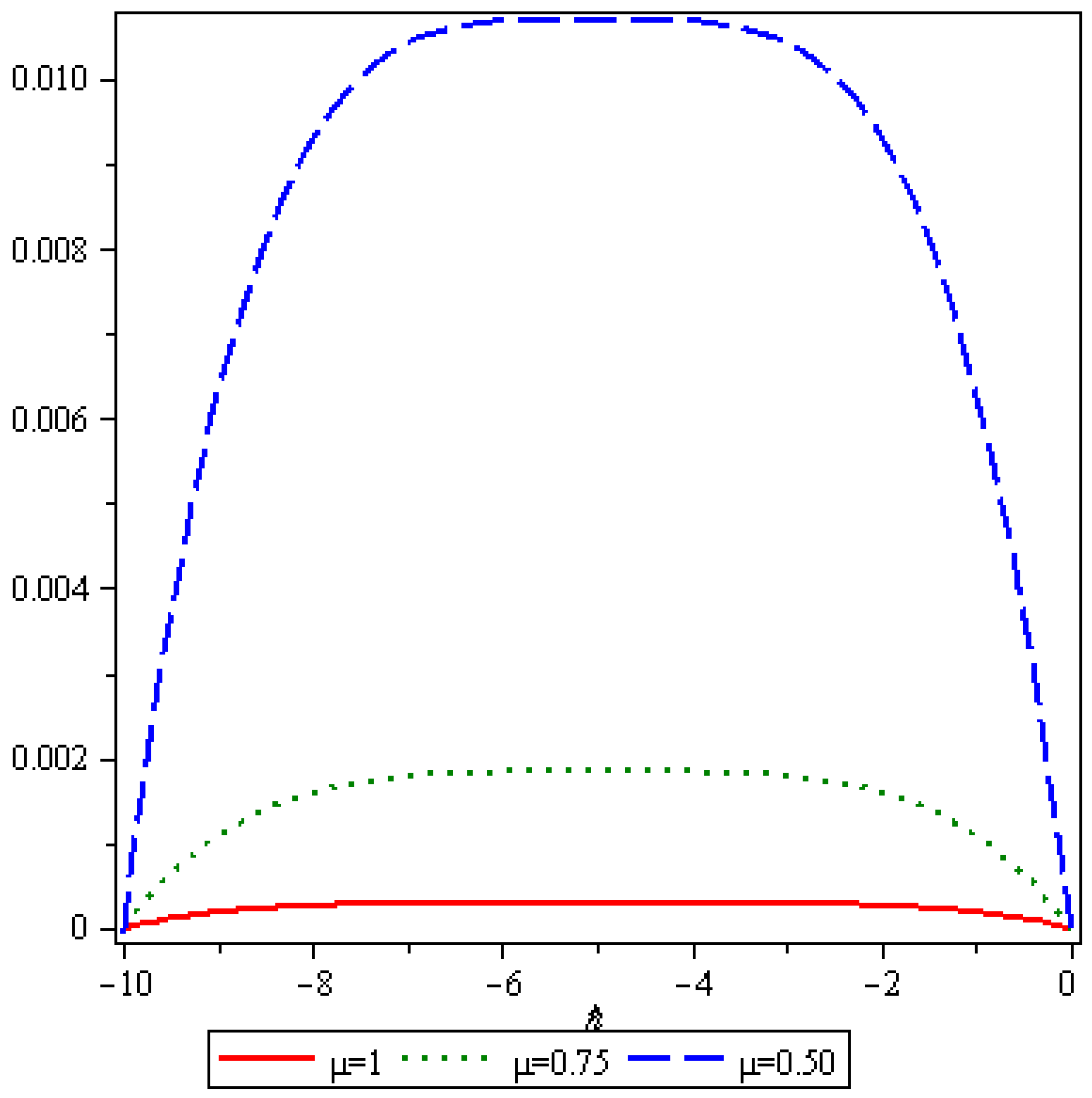
Figure 11.
–curve of for different values of at


Table 1.
Comparative study between q-HASTM and ADM for when = 1, and
| ADM | q-HASTM(for and ) | q-HASTM(for and ) | |
|---|---|---|---|
| 0 | 0 | 0 | 0 |
| 2 | 0.4033806333 | 0.4033788000 | 0.4033790454 |
| 4 | 0.8110188698 | 0.8109674666 | 0.8109706878 |
| 6 | 1.219148908 | 1.218802800 | 1.218817897 |
| 8 | 1.624049986 | 1.622732800 | 1.622778592 |
| 10 | 2.022138493 | 2.018416666 | 2.018525638 |
| 12 | 2.410163488 | 2.401324800 | 2.401546847 |
| 14 | 2.785587314 | 2.766738800 | 2.767144981 |
| 16 | 3.147219587 | 3.109751466 | 3.110437747 |
| 18 | 3.496167079 | 3.425266800 | 3.426357807 |
| 20 | 3.837175265 | 3.708000000 | 3.709652760 |
Table 2.
Comparative study between q-HASTM and ADM for when = 1, and
| ADM | q-HASTM(for and ) | q-HASTM(for and ) | |
|---|---|---|---|
| 0 | 0 | 0 | 0 |
| 2 | 0.5829289274 | 0.5829274000 | 0.5829287007 |
| 4 | 1.134891434 | 1.134838400 | 1.134860301 |
| 6 | 1.659550026 | 1.659119400 | 1.659232190 |
| 8 | 2.159330141 | 2.157414400 | 2.157773939 |
| 10 | 2.635727526 | 2.629625000 | 2.630507313 |
| 12 | 3.089599578 | 3.073910400 | 3.075746263 |
| 14 | 3.521399539 | 3.486687400 | 3.490096920 |
| 16 | 3.931326626 | 3.862630400 | 3.868457617 |
| 18 | 4.319398257 | 4.194671400 | 4.204018861 |
| 20 | 4.685515415 | 4.474000000 | 4.488263354 |
© 2017 by the authors. Licensee MDPI, Basel, Switzerland. This article is an open access article distributed under the terms and conditions of the Creative Commons Attribution (CC BY) license (http://creativecommons.org/licenses/by/4.0/).
Share and Cite
MDPI and ACS Style
Singh, J.; Kumar, D.; Qurashi, M.A.; Baleanu, D. A Novel Numerical Approach for a Nonlinear Fractional Dynamical Model of Interpersonal and Romantic Relationships. Entropy 2017, 19, 375. https://doi.org/10.3390/e19070375
AMA Style
Singh J, Kumar D, Qurashi MA, Baleanu D. A Novel Numerical Approach for a Nonlinear Fractional Dynamical Model of Interpersonal and Romantic Relationships. Entropy. 2017; 19(7):375. https://doi.org/10.3390/e19070375
Chicago/Turabian StyleSingh, Jagdev, Devendra Kumar, Maysaa Al Qurashi, and Dumitru Baleanu. 2017. "A Novel Numerical Approach for a Nonlinear Fractional Dynamical Model of Interpersonal and Romantic Relationships" Entropy 19, no. 7: 375. https://doi.org/10.3390/e19070375
Note that from the first issue of 2016, this journal uses article numbers instead of page numbers. See further details here.