Tidal Analysis Using Time–Frequency Signal Processing and Information Clustering


1
UISPA–LAETA/INEGI, Faculty of Engineering, University of Porto, Rua Dr. Roberto Frias,4200-465 Porto, Portugal
2
Institute of Engineering, Polytechnic of Porto, Department of Electrical Engineering,Rua Dr. António Bernardino de Almeida, 431, 4249-015 Porto, Portugal
*
Author to whom correspondence should be addressed.
Entropy 2017, 19(8), 390; https://doi.org/10.3390/e19080390
Submission received: 11 June 2017
/
Revised: 13 July 2017
/
Accepted: 26 July 2017
/
Published: 29 July 2017
(This article belongs to the Special Issue Wavelets, Fractals and Information Theory III)
Abstract
:Geophysical time series have a complex nature that poses challenges to reaching assertive conclusions, and require advanced mathematical and computational tools to unravel embedded information. In this paper, time–frequency methods and hierarchical clustering (HC) techniques are combined for processing and visualizing tidal information. In a first phase, the raw data are pre-processed for estimating missing values and obtaining dimensionless reliable time series. In a second phase, the Jensen–Shannon divergence is adopted for measuring dissimilarities between data collected at several stations. The signals are compared in the frequency and time–frequency domains, and the HC is applied to visualize hidden relationships. In a third phase, the long-range behavior of tides is studied by means of power law functions. Numerical examples demonstrate the effectiveness of the approach when dealing with a large volume of real-world data.
1. Introduction
Geophysical time series (TS) can be interpreted as the output of multidimensional dynamical systems influenced by many distinct factors at different scales in space and time. In light of Takens’ embedding theorem, these TS can reveal—at least partially—the underlying dynamics of the corresponding systems [1].
Some common properties of geophysical TS are their complex structure, non-linearity, and non-stationarity [2,3]. These characteristics pose difficulties in processing the data that are not easily addressed by means of tools such as Fourier analysis [4,5]. To overcome such limitations, other techniques for spectral estimation are adopted, such as the least-squares [6] and singular spectrum analysis [7], the multitaper method (MM) [8], and the autoregressive moving average [9] and maximum entropy techniques [10]. Alternatively, time–frequency methods [11] have proven powerful for processing non-linear and non-stationary data. We can mention not only the fractional [12,13], short time [14,15], and windowed Fourier [16,17] transforms, but also the Gabor [18,19], wavelet [20,21], Hilbert–Huang [22,23], and S [24,25] transforms. Additionally, distinct complexity measures (e.g., entropy, Lyapunov exponent, Komologrov estimates, and fractal dimension) [26], detrended fluctuation analysis [27], and recurrence plots [28], among others [3,29,30,31,32,33], are also adopted for analyzing complex TS.
Jalón-Rojas et al. [34] compared different spectral methods for the analysis of high-frequency and long TS collected at the Girond estuary. They considered specific evaluation criteria and concluded that the combination of distinct methods could be a good strategy for dealing with data measured at coastal waters. Grinsted et al. [35] adopted the cross wavelet transform and wavelet coherence for examining relationships in time and frequency between two TS. They applied these methods to the Arctic Oscillation index and the Baltic maximum sea ice extent record. Vautard et al. [7] used the singular-spectrum analysis, demonstrating the effectiveness of the technique when dealing with short and noisy TS. Malamud and Turcotte [36] introduced the self-affine TS, characterized by a power spectral density (PSD) that is described by a power law (PL) function of the frequency. They addressed a variety of techniques to quantify the strength of long-range persistence—namely, the Fourier power spectral, semivariogram, rescaled-range, average extreme-event, and wavelet variance analysis. Ding and Chao [9] adopted autoregressive methods for detecting harmonic signals with exponential decay or growth contained in noisy TS. Donelan et al. [10] used the maximum likelihood, maximum entropy, and wavelets for estimating the directional spectra of water waves. Gong et al. [37] adopted the S-transform for analyzing seismic data. Huang et al. [22] proposed empirical mode decomposition and the Hilbert–Huang transform. First, a TS is decomposed into a finite and often small number of intrinsic mode functions, and then the Hilbert transform is applied to the modes. Forootan and Kusche [38] used independent component analysis to separate unknown mixtures of deterministic sinusoids with non-null trend. Doner et al. [39] explored recurrence networks, interpreting the recurrence matrix of a TS as the adjacency matrix of an associated complex network that links different points in time if the considered states are closely neighbored in the phase space. The recurrence matrix yields new quantitative characteristics (such as average path length, clustering coefficient, or centrality measures of the recurrence network) related to the dynamical complexity of the TS. Lopes at al. [32,40,41] investigated geophysical data by means of multidimensional scaling and fractional order techniques.
Tides are variations in the sea level mainly caused by astronomical components, such as gravitational forces exerted by the Moon, the Sun, and the rotation of the Earth, but also reflect non-astronomical sources such as the weather [42]. Understanding the sea-level variations is of great importance for both safe navigation and for planning and promoting the sustainable development of coastal areas. Moreover, sea-level observations provide valuable data to ocean sciences, geodynamics, and geosciences [43,44]. Tides can be measured by means of gauges, with respect to a datum, and the values are recorded over time. A large volume of tidal information is presently available for scientific research. Tidal TS include harmonic constituents and other components with multiple time scales that span from hours to decades. On such time scales, tidal data are often non-stationary, and as with most geophysical TS, standard mathematical tools are insufficient to satisfactorily assess the information that they embed.
In this paper we combine time–frequency methods and hierarchical clustering (HC) techniques to process and visualize tidal information. In a first phase, we pre-process the raw data (i.e., we fill the gaps in the TS with values calculated with a suitable tidal model), and then we normalize the data to obtain dimensionless TS. In a second phase, we use the Jensen–Shannon divergence (JSD) to measure the dissimilarities between TS collected at several stations located worldwide. The TS are compared in the frequency and time–frequency domains. The frequency domain information consists of the PSD generated by the MM. The time–frequency information corresponds to the magnitudes of the fractional Fourier transform (FrFT) and the continuous wavelet transform (CWT) of the TS. In the three cases, HC generates maps that are interpreted based on the emerging clusters of the points that represent tidal stations. In a third phase, the long-range behavior of tides is modeled by means of PL functions using the TS spectra at low frequencies. Numerical examples demonstrate the effectiveness of the approach when dealing with a large volume of real-world data.
In this line of thought, the structure of the paper is as follows. Section 2 presents the main mathematical tools used for processing the TS. Section 3 introduces the data set and the pre-processing used to generate well-formatted TS. Section 4 applies the HC method and discusses the results. Section 5 studies the long-range behavior of tides by means of PL functions. Finally, Section 6 draws the main conclusions.
2. Mathematical Fundamentals
This section introduces the main mathematical tools adopted for data processing; namely, the MM, FrFt, CWT, JSD, and HC techniques. These tools are well-suited to TS generated by most naturally-occurring phenomena, as is the case of biological, climatic, and geophysical processes.
2.1. Multitaper Method
The MM is a robust numerical algorithm for estimating the PSD of a signal. Given an N-length sequence , its PSD can be estimated by the single-taper, or modified periodogram function, , derived directly from the FT of [45]. Therefore, we have:
where t and f denote time and frequency, respectively, and . The function is called a taper, or window, and represents a series of weights that verify the condition . If is a rectangular (or boxcar) function, then (1) yields the standard periodogram of [46].
Expression (1) leads to a biased estimate of the PSD due to both spectral leakage (i.e., power spreading from strong peaks at a given frequency towards neighboring frequencies) and variance of (i.e., noise affecting the spectra). To avoid these artifacts, the MM method was introduced by Thomson [47]. In this method, is multiplied by a set of orthogonal sequences, or tapers, to obtain a set of single-taper periodograms. The set is then averaged to yield an improved estimate of the PSD, , given by:
where , , are spectral estimates, or eigenspectra functions, and are the eigencomponents:
obtained with K Slepian sequences, , that verify [48]:
2.2. Fractional Fourier Transform
The FrFT of order , , is a linear integral operator that maps a given function (or signal) onto , , by the expression [51]:
where, setting , the kernel is defined as:
with
For , , , we should take limiting values. Furthermore, when and , the FrFT becomes and , respectively, and the kernels are:
When , we have that corresponds to the ordinary Fourier transform (FT), and when , we have . Therefore, the operator can be interpreted as the ath power of the ordinary FT, that may be considered modulo 4 [51,52]. For the digital computation of , different algorithms were proposed [51]. Here we adopt the Fast Approximate FrFT [51] (https://nalag.cs.kuleuven.be/research/software/FRFT/). The signal must be evenly sampled and without gaps.
2.3. Wavelet Transform
The wavelet transform converts a given function, , from standard time into the generalized time–frequency domain, and represents a powerful tool for identifying intermittent periodicities in the data. The discrete wavelet transform is particularly useful for noise reduction and data compression, while the CWT is better for feature extraction [35].
The CWT of is given by [53,54,55]:
where denotes the mother wavelet function, represents the complex conjugate of the argument, and the parameters represent the dyadic dilation and translation of , respectively.
The CWT processes data at different scales. The temporal analysis is performed with a contracted version of the prototype wavelet, while frequency analysis is derived with a dilated version of . The parameter a is related to frequency, and b often represents time or space.
The choice of an appropriate mother wavelet represents a key issue in the analysis [53,56]. Some initial knowledge about the signal characteristics is important, but we often choose based on several trials and the results obtained. Therefore, the best is the one that more assertively highlights the features that we are looking for.
Two TS can be compared directly by computing their wavelet coherence as a function of time and frequency. In other words, wavelet coherence measures time-varying correlations as a function of frequency [35,44,57].
Given two TS, and , their wavelet coherence is given by [35,44,58]:
where is a smoothing function in time and frequency.
Similarly to the MM and FrFT, the CWT can be applied to TS evenly sampled and without missing data.
2.4. Jensen–Shannon Divergence
The JSD measures the dissimilarity between two probability distributions, P and Q [59], and is the smoothed and symmetrical version of the Kullback–Leibler divergence, or relative entropy, given by:
The JSD is formulated as:
where is a mixture distribution.
Alternatively, we can write:
2.5. Hierarchichal Clustering
Clustering analysis groups objects that are similar to each other in some sense. In HC, a hierarchy of object clusters is built based on one of two alternative algorithms. In agglomerative clustering, each object starts in its own singleton cluster, and at each step the two most similar clusters are greedily merged. The algorithm stops when all objects are in the same cluster. In divisive clustering, all objects start in one cluster, and at each step the algorithm removes the outsiders from the least cohesive cluster. The iterations stop when each object is in its own singleton cluster. The clusters are combined (split) for agglomerative (divisive) clustering based on their dissimilarity. Therefore, given two clusters, I and J, a metric is specified to measure the distance, , between objects and , and the dissimilarity between clusters, , is calculated by the maximum, minimum, or average linkage, given by:
The results of HC are usually presented in a dendrogram or a tree diagram.
3. Dataset
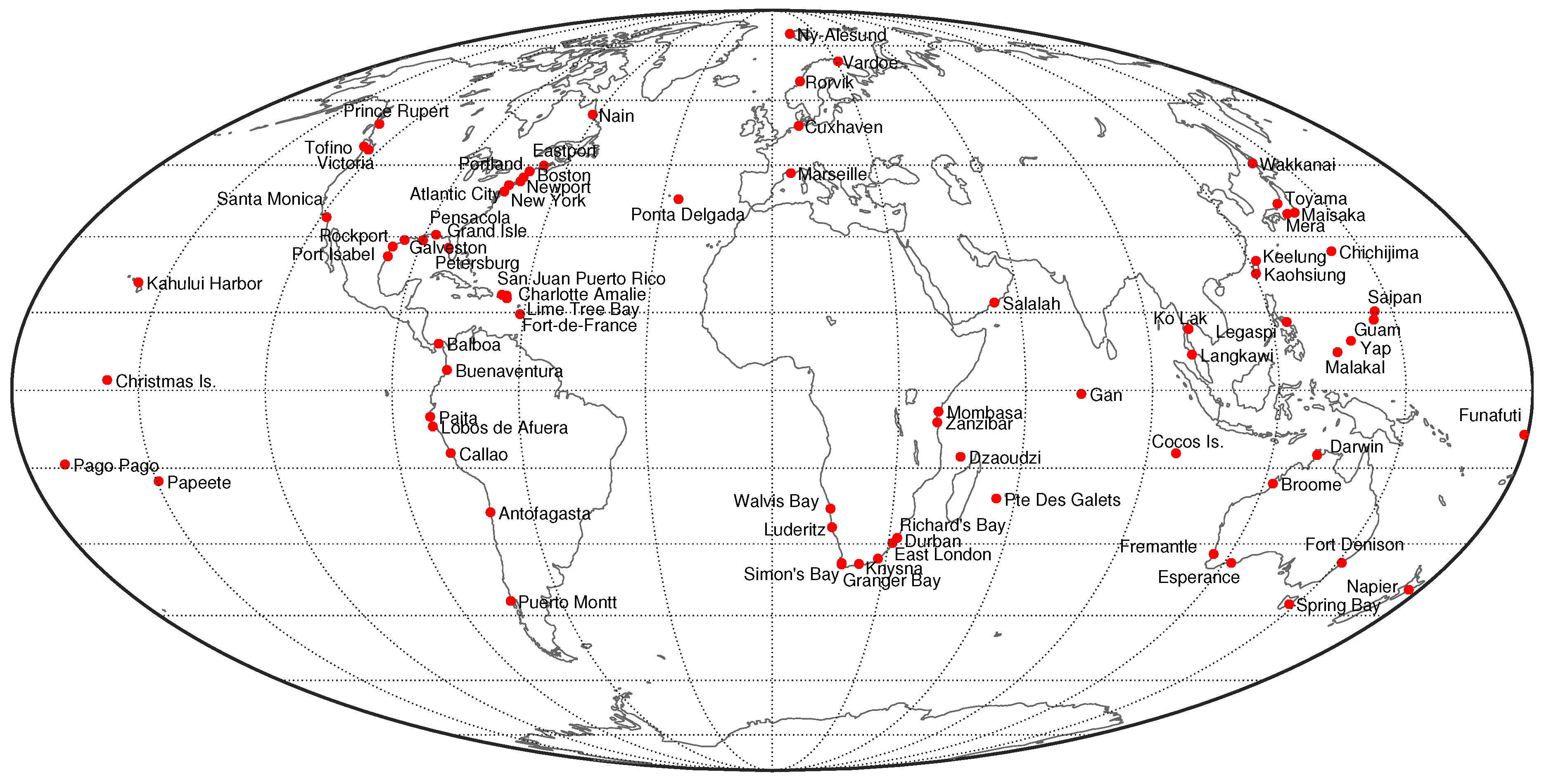
The tidal information are available at the University of Hawaii Sea Level Center (http://uhslc.soest.hawaii.edu/). Worldwide stations have records covering different time periods. We consider hourly data collected between January, 1 1994 and December, 31 2014 at stations. Their labels, names, and percentage of missing data are shown in Table 1. The stations’ geographical location is depicted in Figure 1.
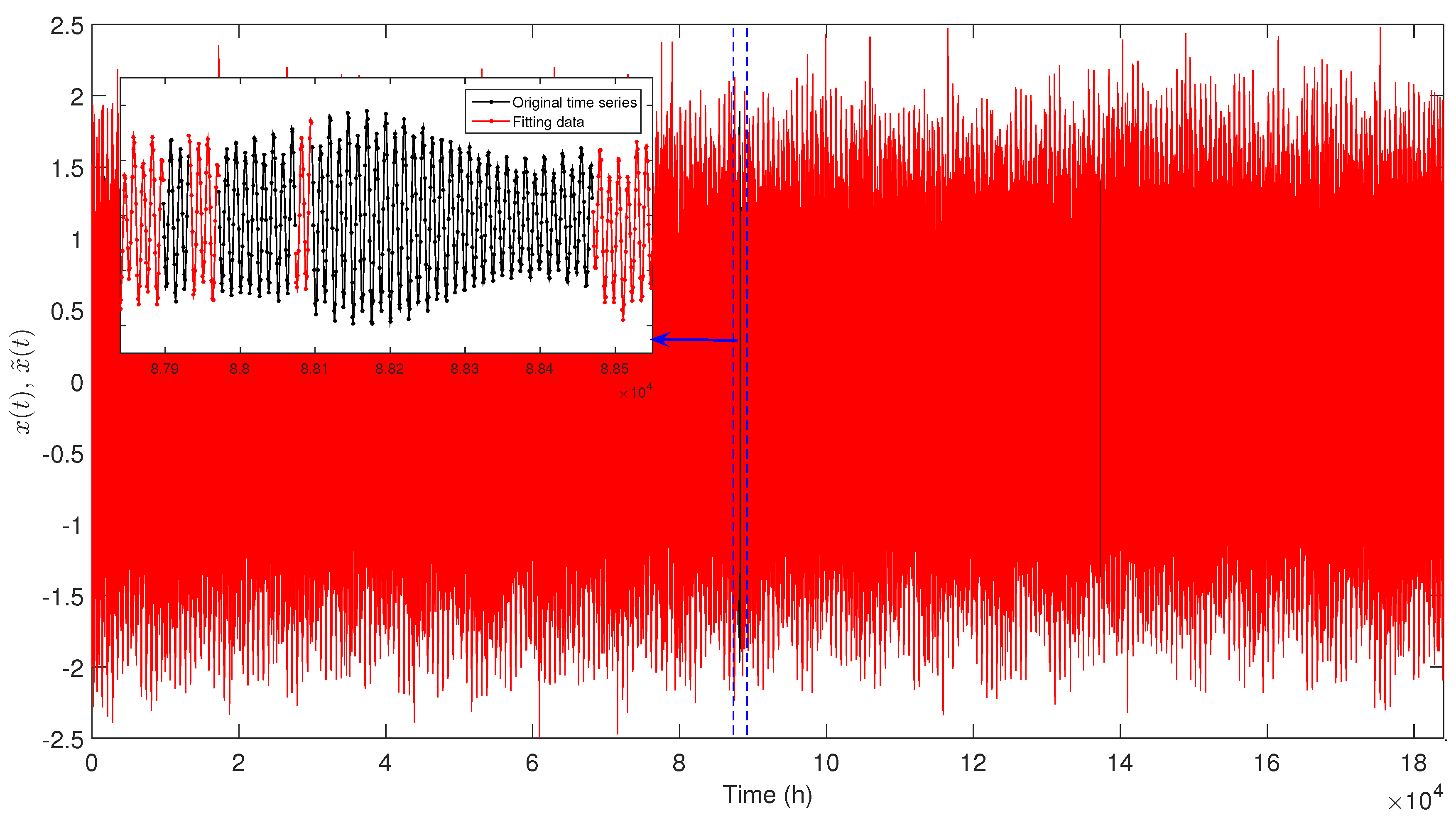
Occasional gaps in the TS, , must be filled before applying the MM and CWT processing tools. The missing values are replaced by artificial data generated by a tidal model, , given by:
where denotes the average value of , and the sinusoidal terms represent standard tidal constituents of known frequency, , , according to the International Hydrographic Organization (https://www.iho.int/srv1/index.php?lang=en). The amplitude and phase shift, and , are computed by the least-squares method.
4. Analysis and Visualization of Tidal Data
In this section, we use HC for visualizing the relationships between tidal TS. The signals, , , are first normalized to zero mean and unit variance in order to get a dimensionless TS:
where and represent the mean and standard deviation values of , respectively.
In SubSection 4.1 and Section 4.2, we use the JSD to measure the dissimilarities between the tidal data in the frequency and time–frequency domains, respectively, and we apply the HC algorithm to visualize relationships. It should be noted that other dissimilarity measures are possible [32,33], but several numerical experiments led to the conclusion that the JSD yields reliable results.
4.1. HC Analysis in the Frequency Domain
Data in the frequency domain corresponds to the TS PSD estimates, , calculated with the MM as defined in (5). The superiority of the MM over the standard periodogram is illustrated in Figure 3 for data collected at the Boston tidal station (lat: , lon: ). We observe that the variance (spectral noise) of is considerably smaller than the one obtained for the classical periodogram, . We obtain similar results for other tidal stations.
We normalize the PSD estimates, , by calculating the ratio:
where is interpreted as a probability distribution [60], and we feed the HC with the matrix , , where represents the JDS between the normalized PSD estimates . Figure 4 depicts the tree generated by applying the successive (agglomerative) and average-linkage methods [32,40]. The software PHYLIP was used for generating the graph [61].
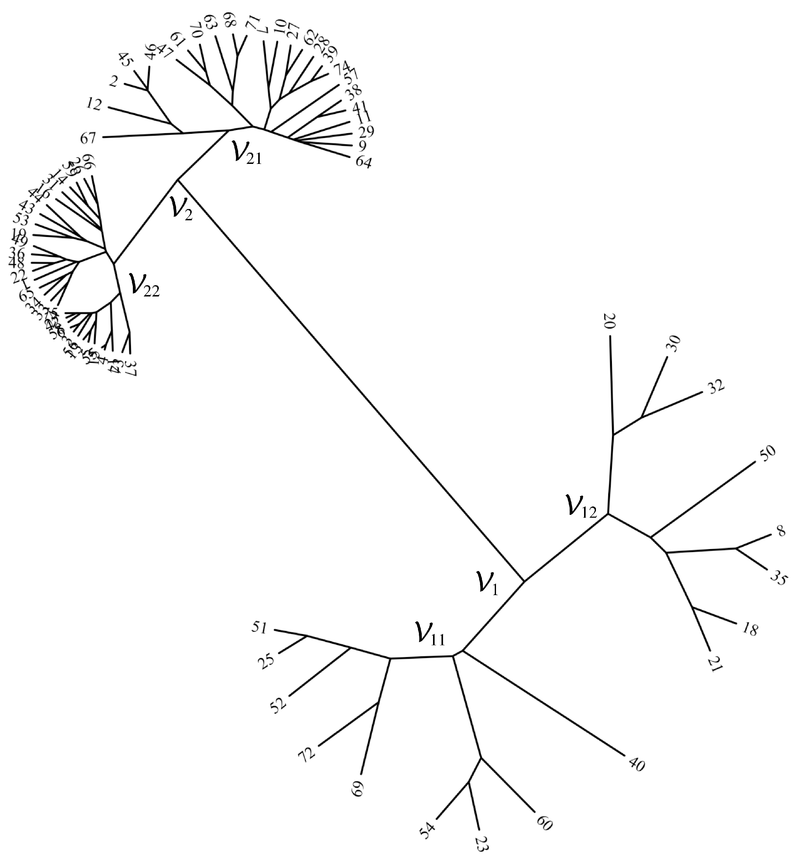
We observe not only the emergence of two main (level 1) clusters, and , but also the presence of various sub-clusters at different lower levels. For example, cluster is composed of level 2 sub-clusters and , while comprises , , and the “outlier” station 50. Nevertheless, at lower levels of the hierarchical tree, the elements of certain sub-clusters emerge very close to each other, making visualization more difficult.
4.2. HC Analysis in the Time–Frequency Domain
4.2.1. The FFrT-Based Approach
The FrFT converts a function to a continuum of intermediate domains between the orthogonal time (or space) and frequency domains. Therefore, it can be thought of as an operator that rotates a signal by any angle, instead of just radians as performed by the ordinary FT.
Figure 5 depicts the log magnitude of the FrFT versus parameter and h for Boston (lat: , lon: ) and Christmas Is. (lat: , lon: ) tidal stations. For , the FrFT corresponds to the time domain signal. For , the FrFT yields the ordinary FT. The main peaks observed in the time domain propagate along the continuum of pseudofrequency (or time–frequency) domains (as a increases), originating high-energy paths that determine the shape of the FrFT charts. Close to (i.e., to half of the total number of samples of the TS), we observe a high-energy component that corresponds to the DC frequency, but other details are difficult to perceive. We obtain similar patterns for other tidal stations.
The structure of the FrFT plots reflect the characteristics of the TS. Nevertheless, to the authors best knowledge, there are not yet assertive tools to explore this three-dimensional information.
For each TS, we calculate the corresponding FrFT, and we generate an dimensional complex-valued matrix, W, where L and N denote the number of points in frequency and time, respectively. We then compute the dimensional vector , , composed of the columns of , and we perform the normalization:
where the function is interpreted as a probability distribution. Finally, we feed the HC with the matrix , , where represents the JSD between the normalized vectors .
Figure 6 depicts the tree generated by the HC. As before, the successive (agglomerative) and average-linkage methods were used [32,40]. We observe two main clusters, and , that are similar to the ones identified by the MM-based approach, and , respectively, revealing good consistency between the two processing alternatives.
4.2.2. The CWT-Based Approach
The CWT is well suited to non-stationary signals and establishes a compromise between precision analysis in the time and frequency domains [62]. We adopt here the complex Morlet wavelet, since several numerical experiments were revealed to be a good choice in the context of continuous analysis and feature extraction [35,44]. The complex Morlet wavelet is defined as:
where is related to the wavelet bandwidth and is its center frequency. These constants can be interpreted as the parameters of a time-localized filtering, or correlation, operator.
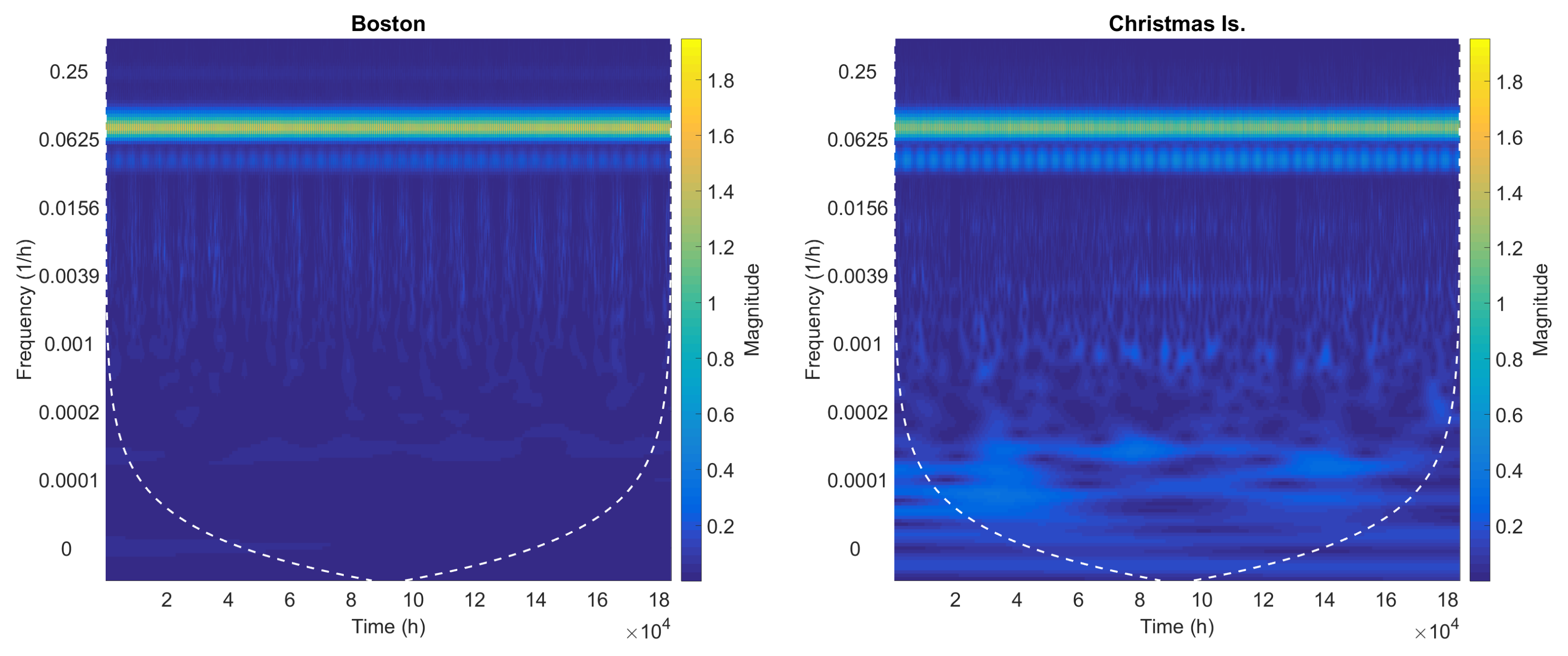
Figure 7 depicts the CWT for Boston (lat: , lon: ) and Christmas Is. (lat: , lon: ) tidal stations. We observe two main patterns at frequencies around and , corresponding to the semi-diurnal and diurnal tidal components, but other objects are difficult to identify. For other tidal stations we obtain similar patterns.
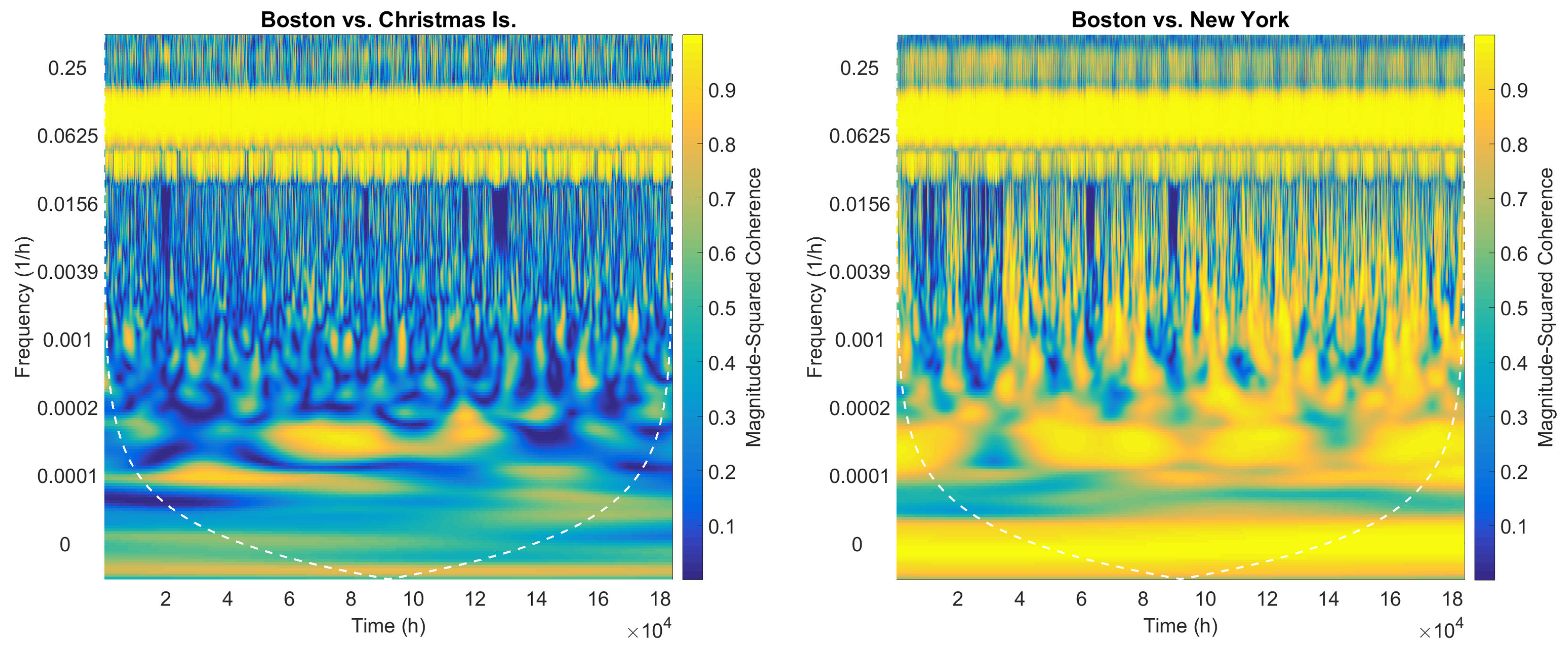
Figure 8 shows the similarities between the two station pairs Boston (lat: , lon: ) vs. Christmas Is. (lat: , lon: ) and Boston (lat: , lon: ) vs. New York (lat: , lon: ). That is, we present one pair of distant and one pair of neighbor stations. We verify that coherence between neighbors is higher and—as expected—we observe regions of strong coherence at the frequencies of the main tidal components (Table 2). However, other strong coherence regions emerge throughout the data which are difficult to infer from the bare CWT charts. Therefore, from Figure 8 we conclude that wavelet coherence is a powerful tool for unveiling hidden similarities between data. Yet, since it produces one chart per TS pair, a large amount of data is generated for all combinations of pairs, and the global perspective is difficult to obtain. To overcome these problems, in the follow up, we combine CWT and HC tools.
For all TS, we determine the corresponding CWT, and as described in SubSection 4.2.1, we calculate the function , where now denotes a vector obtained from , with W generated by the CWT. Finally, we feed the HC with the matrix , .
Figure 9 depicts the tree generated for matrix . We observe two main clusters, and , that are similar to those already identified in the MM- and FrFT-based trees. For example, relative to and , the main differences are for stations 30 (Keelung) and 50 (Papeete), which swapped places. Sub-clusters at lower levels are now well separated, demonstrating the superiority of the time–frequency analysis in discriminating differences between the data.
In conclusion, the trees from Figure 4, Figure 5, Figure 6, Figure 7, Figure 8 and Figure 9 reveal the same type of clusters, with slightly distinct levels of discrimination of the sub-clusters, Figure 9 apparently being slightly superior to the others. This global comparison shows that geographically close stations can behave differently from each other due to local factors. However, this may be not perceived when using standard processing tools.
5. Long-Range Behavior of Tides
The previous analysis revealed similarities embedded into distinct TS, but does not focus on long memory effects that often occur in complex systems. Having this fact in mind, in this section we study the long-range behavior of tides based on the characteristics of the TS PSD at low frequencies. Therefore, we model the MM estimates, , , within the bandwidth , where and denote the lower and upper frequency limits by means of PL functions:
In this perspective, “low frequencies” means the bandwidth bellow the first harmonics with significant amplitude; that is, .
The values obtained for parameter b reveal underlying characteristics of the tidal dynamics; namely, a fractional value of b may be indicative of dynamical properties similar to those usually found in fractional-order systems [41,63,64]. Moreover, Equation (23) implies a relationship between PL behavior and fractional Brownian motion (fBm) [30,65] ( noise [66]), since for many systems fBm represents a signature of complexity [67].
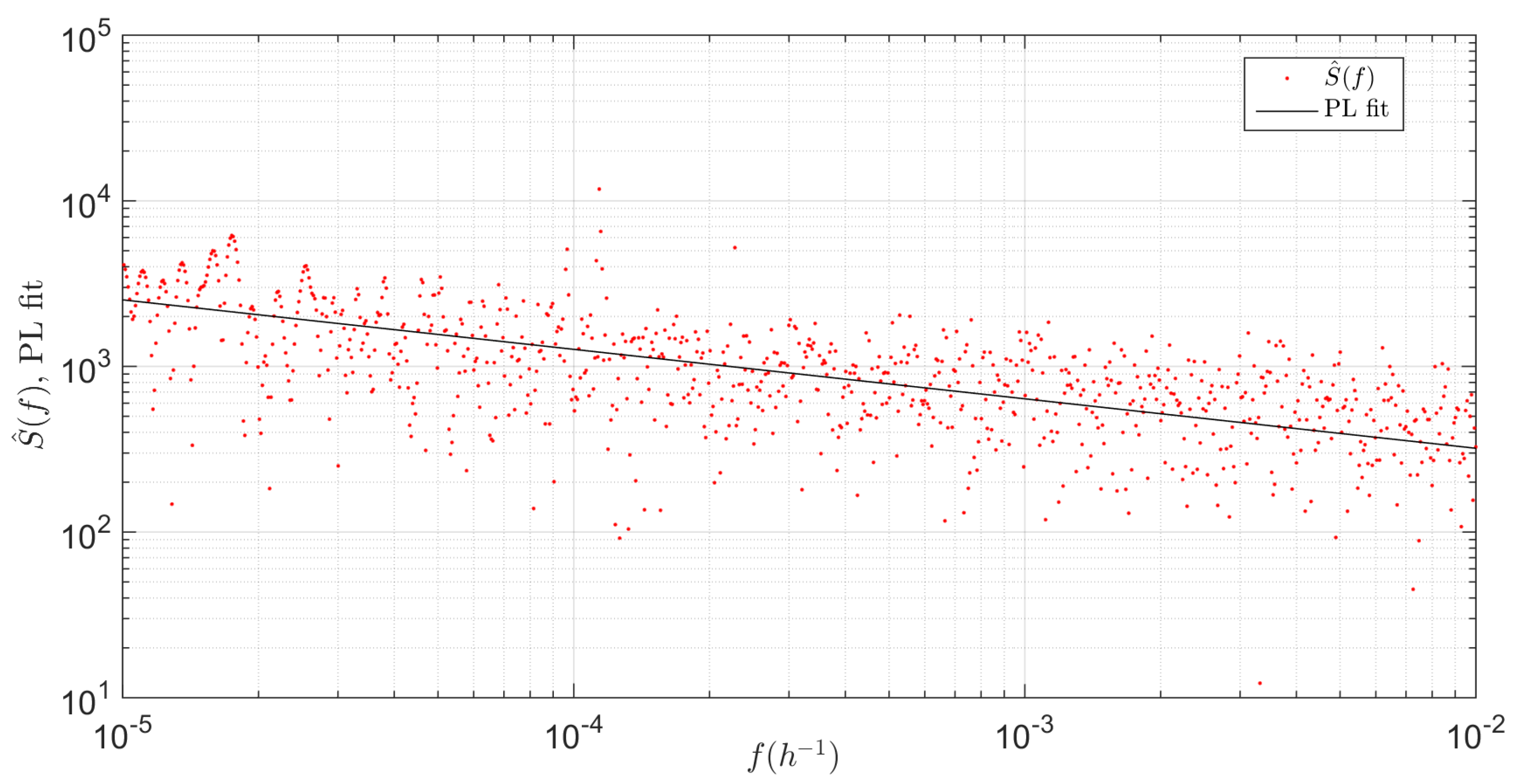
Figure 10 illustrates the procedure for data from the Boston tidal station (lat: , lon: ), (i.e., 4 days to 11.5 years), and the PL parameters determined by means of least squares fitting, yielding .
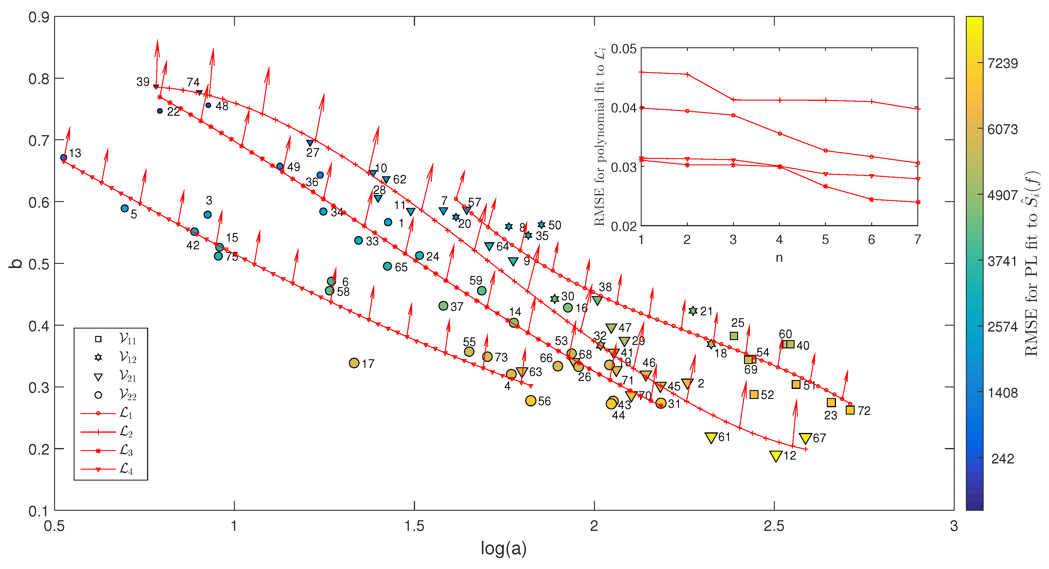
The parameters are computed for the whole set of time-series ( in total), and the corresponding locus is depicted in Figure 11. The size and color of the markers are proportional to the value of the root mean squared error (RMSE) of the PL fit. We verify that b has values between 0.2 and 0.8, corresponding to TS including long memory effects typical of fBm. Values of b close to zero mean that tidal TS are close to white noise; that is, to a random signal having equal intensity at different frequencies. On the other hand, values of b close to 1 follow the so-called pink or noise, which occurs in many physical and biological systems. In general, for non-integer values of b, signals are related to the ubiquitous fractional Brownian noise. So, we can say loosely that the smaller/higher the values of b, the less/more correlated are consecutive signal samples and the smaller/larger is the content of long-range memory effects.
In Figure 11, we group points in the locus into four clusters , , loosely having the correspondence , , and . Therefore, we find that the clusters previously identified with the tree diagrams for the global time scale have a distinct arrangement in the long-range perspective. The chart also includes the approximation curves to , , yielding lines resembling isoclines in a vector field. Third-order polynomials (i.e., degree ) were interpolated since they lead to a good compromise between reducing the RMSE of the fit and avoiding overfitting. From the gradient generated by the isoclines approximation, we observe not only a gradual and smooth evolution between the four isoclines, but also a clear separation between them, with particular emphasis on and . This property was not clear in the previous diagram trees. Long-range memory effects are diluted when handling TS simultaneously with long and short time scales, but the locus unveils properties that reflect distinct classes of phenomena, and their identification needs further study.
We should also note that the low-frequency range covers time scales between 1 year and several decades. So, the results demonstrate the presence of phenomena influencing tides during long periods of time. The limits of such time scales remain to be explored, since present-day TS do not include sufficiently long records. In other words, the results point toward obtaining longer TS, since relevant phenomena may be not completely captured with the available data.
6. Conclusions
Tidal TS embed rich information contributed by a plethora of factors at different scales. Local features—namely, geography (e.g., shape of the shoreline, bays, estuaries, and inlets, presence of shallow waters) and weather (e.g., wind, atmospheric pressure, and rainfall/river discharge)—may have a non-negligible effect on tides. This means that, for example, geographically close stations may register quite different tidal behavior. Knowing the relationships between worldwide distributed stations may be important to better understanding tides. However, disclosing such relationships requires powerful tools for TS analysis that are able to unveil all details embedded in the data.
A method for analyzing tidal TS that combines time–frequency signal processing and HC was proposed. Real world information from worldwide tidal stations was pre-processed to obtain TS with reliable quality. Frequency and time–frequency data were generated by means of the MM, FrFT, and CWT. The JSD was used to measure dissimilarities, and the HC was applied for visualizing information. PL functions were adopted for investigating the long-range dynamics of tides. Numerical analysis showed that the combination of CWT and HC leads to a good graphical representation of the relationships between tidal TS. The two distinct perspectives of study reveal similar regularities embedded into the raw TS and motivate their adoption with other geophysical information.
Acknowledgments
The authors acknowledge the University of Hawaii Sea Level Center (http://uhslc.soest.hawaii.edu/) for the data used in this paper. This work was partially supported by FCT (“Fundção para a Ciência e Tecnologia, Portugal”) funding agency, under the reference Projeto LAETA – UID/EMS/50022/2013.
Author Contributions
These authors contributed equally to this work.
Conflicts of Interest
The authors declare no conflict of interest.
References
- Takens, F. Detecting Strange Attractors in Turbulence. In Dynamical Systems and Turbulence, Warwick 1980; Springer: Berlin, Germany, 1981; pp. 366–381. [Google Scholar]
- Dergachev, V.A.; Gorban, A.; Rossiev, A.; Karimova, L.; Kuandykov, E.; Makarenko, N.; Steier, P. The filling of gaps in geophysical time series by artificial neural networks. Radiocarbon 2001, 43, 365–371. [Google Scholar]
- Ghil, M.; Allen, M.; Dettinger, M.; Ide, K.; Kondrashov, D.; Mann, M.; Robertson, A.W.; Saunders, A.; Tian, Y.; Varadi, F.; Yiou, P. Advanced spectral methods for climatic time series. Rev. Geophys. 2002, 40, 1–41. [Google Scholar]
- Stein, E.M.; Shakarchi, R. Fourier Analysis: An Introduction; Princeton University Press: Princeton, NJ, USA, 2003. [Google Scholar]
- Dym, H.; McKean, H. Fourier Series and Integrals; Academic Press: San Diego, CA, USA, 1972. [Google Scholar]
- Wu, D.L.; Hays, P.B.; Skinner, W.R. A least squares method for spectral analysis of space-time series. J. Atmos. Sci. 1995, 52, 3501–3511. [Google Scholar] [CrossRef]
- Vautard, R.; Yiou, P.; Ghil, M. Singular-spectrum analysis: A toolkit for short, noisy chaotic signals. Phys. D Nonlinear Phenom. 1992, 58, 95–126. [Google Scholar] [CrossRef]
- Thomson, D.J. Multitaper analysis of nonstationary and nonlinear time series data. In Nonlinear and Nonstationary Signal Processing; Cambridge University Press: London, UK, 2000; pp. 317–394. [Google Scholar]
- Ding, H.; Chao, B.F. Detecting harmonic signals in a noisy time-series: The z-domain Autoregressive (AR-z) spectrum. Geophys. J. Int. 2015, 201, 1287–1296. [Google Scholar] [CrossRef]
- Donelan, M.; Babanin, A.; Sanina, E.; Chalikov, D. A comparison of methods for estimating directional spectra of surface waves. J. Geophys. Res. Oceans 2015, 120, 5040–5053. [Google Scholar] [CrossRef]
- Cohen, L. Time-Frequency Analysis; Prentice-Hall: Upper Saddle River, NJ, USA, 1995. [Google Scholar]
- Almeida, L.B. The fractional Fourier transform and time–frequency representations. IEEE Trans. Signal Process. 1994, 42, 3084–3091. [Google Scholar] [CrossRef]
- Sejdić, E.; Djurović, I.; Stanković, L. Fractional Fourier transform as a signal processing tool: An overview of recent developments. Signal Process. 2011, 91, 1351–1369. [Google Scholar]
- Portnoff, M. Time-frequency representation of digital signals and systems based on short-time Fourier analysis. IEEE Trans. Acoust. Speech Signal Process. 1980, 28, 55–69. [Google Scholar]
- Qian, S.; Chen, D. Joint time-frequency analysis. IEEE Signal Process. Mag. 1999, 16, 52–67. [Google Scholar]
- Kemao, Q. Windowed Fourier transform for fringe pattern analysis. Appl. Opt. 2004, 43, 2695–2702. [Google Scholar] [CrossRef] [PubMed]
- Hlubina, P.; Luňáček, J.; Ciprian, D.; Chlebus, R. Windowed Fourier transform applied in the wavelength domain to process the spectral interference signals. Opt. Commun. 2008, 281, 2349–2354. [Google Scholar] [CrossRef] [Green Version]
- Qian, S.; Chen, D. Discrete Gabor Transform. IEEE Trans. Signal Process. 1993, 41, 2429–2438. [Google Scholar] [CrossRef]
- Yao, J.; Krolak, P.; Steele, C. The generalized Gabor transform. IEEE Trans. Image Process. 1995, 4, 978–988. [Google Scholar] [PubMed]
- Mallat, S. A Wavelet Tour of Signal Processing; Academic Press: Burlington, VT, USA, 1999. [Google Scholar]
- Yan, R.; Gao, R.X.; Chen, X. Wavelets for fault diagnosis of rotary machines: A review with applications. Signal Process. 2014, 96, 1–15. [Google Scholar] [CrossRef]
- Huang, N.E.; Shen, Z.; Long, S.R.; Wu, M.C.; Shih, H.H.; Zheng, Q.; Yen, N.C.; Tung, C.C.; Liu, H.H. The empirical mode decomposition and the Hilbert spectrum for nonlinear and non-stationary time series analysis. Proc. R. Soc. Lond. A Math. Phys. Eng. Sci. 1998, 454, 903–995. [Google Scholar] [CrossRef]
- Wu, Z.; Huang, N.E. Ensemble empirical mode decomposition: A noise-assisted data analysis method. Adv. Adapt. Data Anal. 2009, 1, 1–41. [Google Scholar] [CrossRef]
- Zayed, A.I. Hilbert transform associated with the fractional Fourier transform. IEEE Signal Process. Lett. 1998, 5, 206–208. [Google Scholar] [CrossRef]
- Peng, Z.; Peter, W.T.; Chu, F. A comparison study of improved Hilbert–Huang transform and wavelet transform: Application to fault diagnosis for rolling bearing. Mech. Syst. Signal Process. 2005, 19, 974–988. [Google Scholar] [CrossRef]
- Olsson, J.; Niemczynowicz, J.; Berndtsson, R. Fractal analysis of high-resolution rainfall time series. J. Geophys. Res. Atmos. 1993, 98, 23265–23274. [Google Scholar] [CrossRef]
- Matsoukas, C.; Islam, S.; Rodriguez-Iturbe, I. Detrended fluctuation analysis of rainfall and streamflow time series. J. Geophys. Res. 2000, 105, 29165–29172. [Google Scholar] [CrossRef]
- Marwan, N.; Donges, J.F.; Zou, Y.; Donner, R.V.; Kurths, J. Complex network approach for recurrence analysis of time series. Phys. Lett. A 2009, 373, 4246–4254. [Google Scholar] [CrossRef]
- Donner, R.V.; Donges, J.F. Visibility graph analysis of geophysical time series: Potentials and possible pitfalls. Acta Geophys. 2012, 60, 589–623. [Google Scholar] [CrossRef]
- Machado, J.T. Fractional order description of DNA. Appl. Math. Model. 2015, 39, 4095–4102. [Google Scholar] [CrossRef]
- Lopes, A.M.; Machado, J.T. Integer and fractional-order entropy analysis of earthquake data series. Nonlinear Dyn. 2016, 84, 79–90. [Google Scholar] [CrossRef]
- Machado, J.A.T.; Lopes, A.M. Analysis and visualization of seismic data using mutual information. Entropy 2013, 15, 3892–3909. [Google Scholar] [CrossRef]
- Machado, J.A.; Mata, M.E.; Lopes, A.M. Fractional state space analysis of economic systems. Entropy 2015, 17, 5402–5421. [Google Scholar] [CrossRef]
- Jalón-Rojas, I.; Schmidt, S.; Sottolichio, A. Evaluation of spectral methods for high-frequency multiannual time series in coastal transitional waters: Advantages of combined analyses. Limnol. Oceanogr. Methods 2016, 14, 381–396. [Google Scholar] [CrossRef]
- Grinsted, A.; Moore, J.C.; Jevrejeva, S. Application of the cross wavelet transform and wavelet coherence to geophysical time series. Nonlinear Process. Geophys. 2004, 11, 561–566. [Google Scholar] [CrossRef]
- Malamud, B.D.; Turcotte, D.L. Self-affine time series: I. Generation and analyses. Adv. Geophys. 1999, 40, 1–90. [Google Scholar]
- Gong, D.; Feng, L.; Li, X.T.; Zhao, J.-M.; Liu, H.-B.; Wang, X.; Ju, C.-H. The Application of S-transform Spectrum Decomposition Technique in Extraction of Weak Seismic Signals. Chin. J. Geophys. 2016, 59, 43–53. [Google Scholar] [CrossRef]
- Forootan, E.; Kusche, J. Separation of deterministic signals using independent component analysis (ICA). Stud. Geophys. Geod. 2013, 57, 17–26. [Google Scholar] [CrossRef]
- Donner, R.V.; Zou, Y.; Donges, J.F.; Marwan, N.; Kurths, J. Recurrence networks—A novel paradigm for nonlinear time series analysis. New J. Phys. 2010, 12, 033025. [Google Scholar] [CrossRef]
- Lopes, A.M.; Machado, J.T. Analysis of temperature time-series: Embedding dynamics into the MDS method. Commun. Nonlinear Sci. Numer. Simul. 2014, 19, 851–871. [Google Scholar] [CrossRef]
- Machado, J.T.; Lopes, A.M. The persistence of memory. Nonlinear Dyn. 2015, 79, 63–82. [Google Scholar] [CrossRef]
- Pugh, D.; Woodworth, P. Sea-Level Science: Understanding Tides, Surges, Tsunamis and Mean Sea-Level Changes; Cambridge University Press: Cambridge, UK, 2014. [Google Scholar]
- Shankar, D. Seasonal cycle of sea level and currents along the coast of India. Curr. Sci. 2000, 78, 279–288. [Google Scholar]
- Erol, S. Time-frequency analyses of tide-gauge sensor data. Sensors 2011, 11, 3939–3961. [Google Scholar] [CrossRef] [PubMed]
- Brigham, E.O. The Fast Fourier Transform and Its Applications; Number 517.443; Prentice Hall: Upper Sadlle River, NJ, USA, 1988. [Google Scholar]
- Prieto, G.; Parker, R.; Thomson, D.; Vernon, F.; Graham, R. Reducing the bias of multitaper spectrum estimates. Geophys. J. Int. 2007, 171, 1269–1281. [Google Scholar] [CrossRef]
- Thomson, D.J. Spectrum estimation and harmonic analysis. Proc. IEEE 1982, 70, 1055–1096. [Google Scholar] [CrossRef]
- Slepian, D. Prolate spheroidal wave functions, Fourier analysis, and uncertainty–V: The discrete case. Bell Labs Tech. J. 1978, 57, 1371–1430. [Google Scholar] [CrossRef]
- Fodor, I.K.; Stark, P.B. Multitaper spectrum estimation for time series with gaps. IEEE Trans. Signal Process. 2000, 48, 3472–3483. [Google Scholar]
- Smith-Boughner, L.; Constable, C. Spectral estimation for geophysical time-series with inconvenient gaps. Geophys. J. Int. 2012, 190, 1404–1422. [Google Scholar] [CrossRef]
- Bultheel, A.; Sulbaran, H.E.M. Computation of the fractional Fourier transform. Appl. Comput. Harmon. Anal. 2004, 16, 182–202. [Google Scholar] [CrossRef] [Green Version]
- Ozaktas, H.M.; Zalevsky, Z.; Kutay, M.A. The Fractional Fourier Transform; Wiley: Chichester, UK, 2001. [Google Scholar]
- Machado, J.T.; Costa, A.C.; Quelhas, M.D. Wavelet analysis of human DNA. Genomics 2011, 98, 155–163. [Google Scholar] [CrossRef] [PubMed]
- Cattani, C. Wavelet and Wave Analysis as Applied to Materials with Micro or Nanostructure; World Scientific: Singapore, 2007; Volume 74. [Google Scholar]
- Stark, H.G. Wavelets and Signal Processing: An Application-Based Introduction; Springer Science & Business Media: New York, NY, USA, 2005. [Google Scholar]
- Ngui, W.K.; Leong, M.S.; Hee, L.M.; Abdelrhman, A.M. Wavelet analysis: Mother wavelet selection methods. Appl. Mech. Mater. 2013, 393, 953–958. [Google Scholar] [CrossRef]
- Cui, X.; Bryant, D.M.; Reiss, A.L. NIRS-based hyperscanning reveals increased interpersonal coherence in superior frontal cortex during cooperation. Neuroimage 2012, 59, 2430–2437. [Google Scholar] [CrossRef] [PubMed]
- Jeong, D.H.; Kim, Y.D.; Song, I.U.; Chung, Y.A.; Jeong, J. Wavelet Energy and Wavelet Coherence as EEG Biomarkers for the Diagnosis of Parkinson’s Disease-Related Dementia and Alzheimer’s Disease. Entropy 2015, 18, 8. [Google Scholar] [CrossRef]
- Cover, T.M.; Thomas, J.A. Elements of Information Theory; John Wiley & Sons: Hoboken, NJ, USA, 2012. [Google Scholar]
- Sato, A.H. Frequency analysis of tick quotes on the foreign exchange market and agent-based modeling: A spectral distance approach. Phys. A Stat. Mech. Appl. 2007, 382, 258–270. [Google Scholar] [CrossRef]
- Felsenstein, J. PHYLIP (Phylogeny Inference Package) version 3.6. Distributed by the author. Department of Genome Sciences, University of Washington, Seattle. Available online: http://evolution.genetics.washington.edu/phylip.html (accessed on 29 July 2017).
- Tenreiro Machado, J.; Duarte, F.B.; Duarte, G.M. Analysis of stock market indices with multidimensional scaling and wavelets. Math. Probl. Eng. 2012, 2012, 819503. [Google Scholar] [CrossRef]
- Lopes, A.M.; Machado, J.A.T. Fractional order models of leaves. J. Vib. Control 2014, 20, 998–1008. [Google Scholar] [CrossRef]
- Baleanu, D. Fractional Calculus: Models and Numerical Methods; World Scientific: Singapore, 2012; Volume 3. [Google Scholar]
- Mandelbrot, B.B.; Van Ness, J.W. Fractional Brownian motions, fractional noises and applications. SIAM Rev. 1968, 10, 422–437. [Google Scholar] [CrossRef]
- Keshner, M.S. 1/f noise. Proc. IEEE 1982, 70, 212–218. [Google Scholar] [CrossRef]
- Mandelbrot, B.B. The Fractal Geometry of Nature; Macmillan: London, UK, 1983; Volume 173. [Google Scholar]
Figure 1.
Geographic location of the stations considered in the study.

Figure 2.
Original, , and the reconstructed, , time series (TS) of Boston.

Figure 3.
The power spectral density (PSD) for Boston tidal TS calculated through the classical periodogram, , and multitaper method (MM) .
Figure 3.
The power spectral density (PSD) for Boston tidal TS calculated through the classical periodogram, , and multitaper method (MM) .

Figure 4.
The hierarchical tree resulting from , , with , and calculated based on the MM. JSD: Jensen–Shannon divergence.
Figure 4.
The hierarchical tree resulting from , , with , and calculated based on the MM. JSD: Jensen–Shannon divergence.
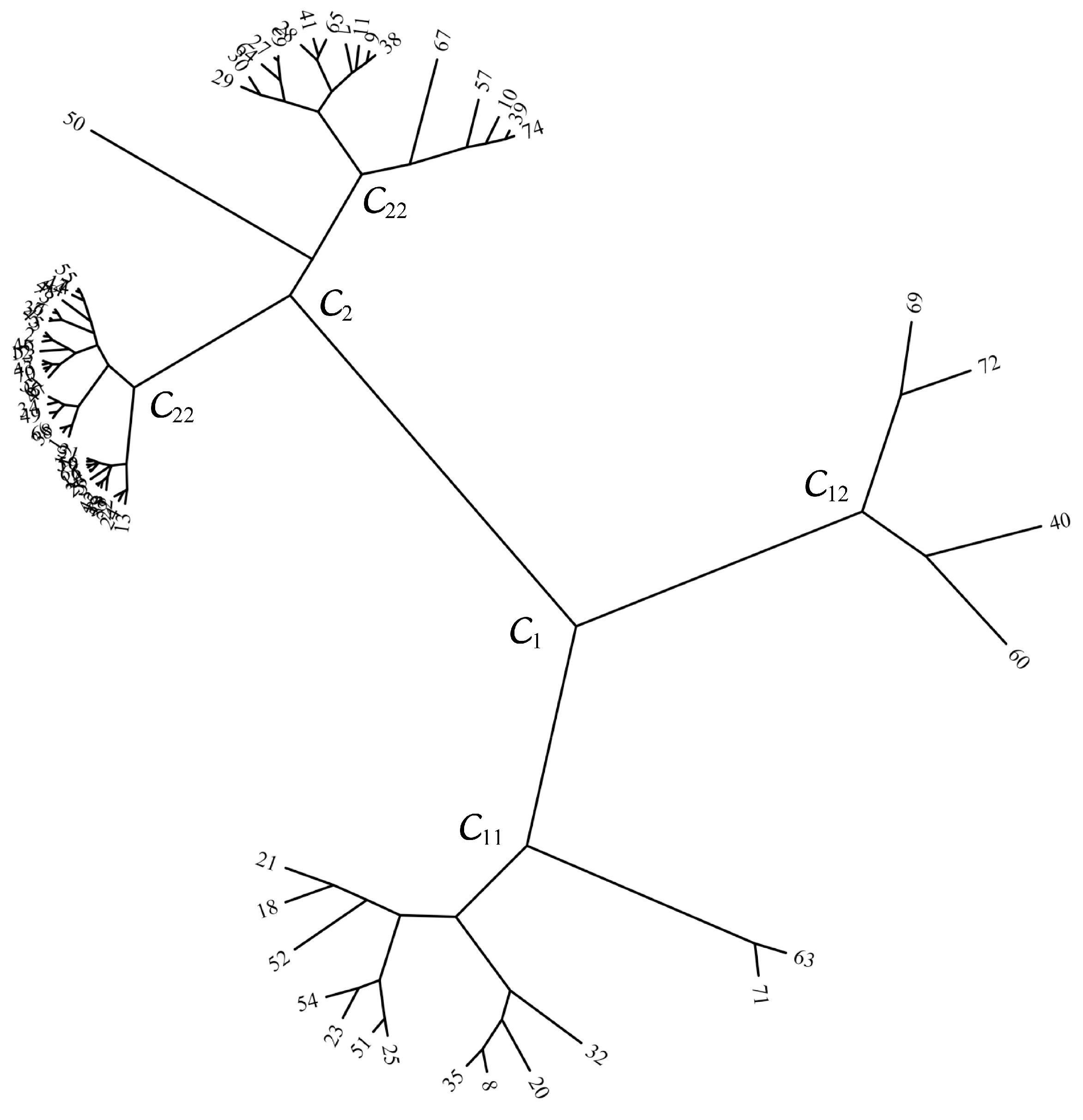
Figure 5.
Locus of magnitude of the fractional Fourier transform (FrFT) (in log scale) versus () for Boston (lat: , lon: ) and Christmas Is. (lat: , lon: ) tidal stations.
Figure 5.
Locus of magnitude of the fractional Fourier transform (FrFT) (in log scale) versus () for Boston (lat: , lon: ) and Christmas Is. (lat: , lon: ) tidal stations.
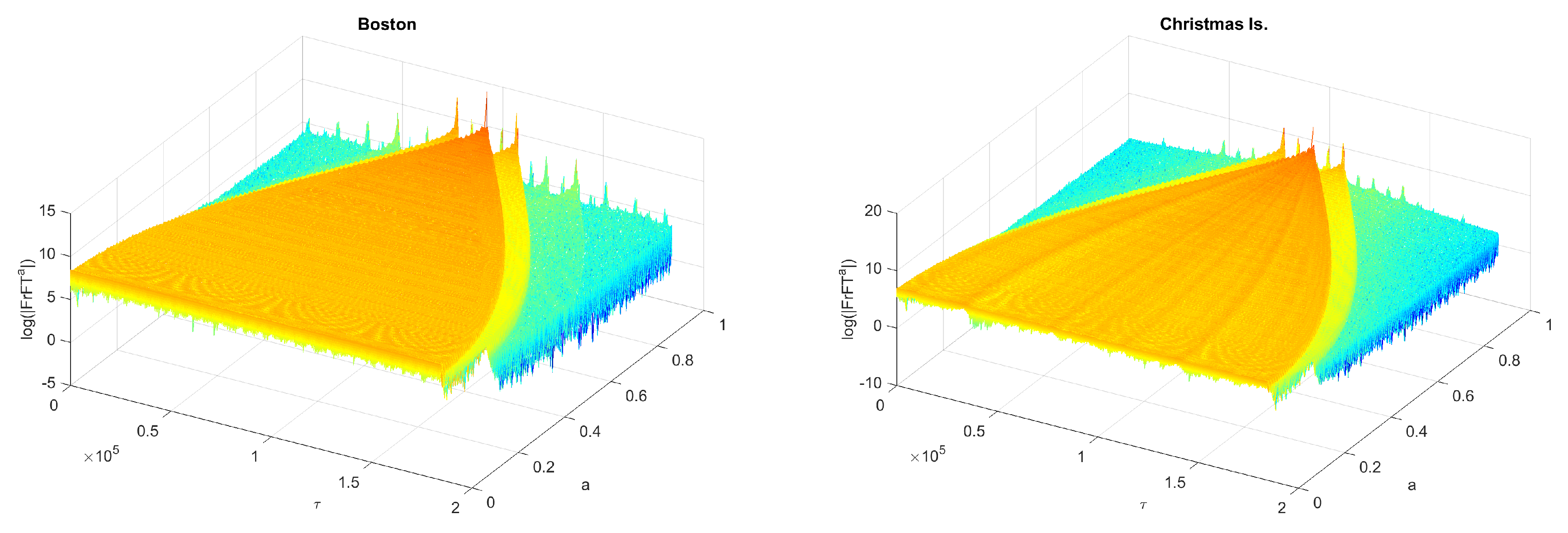
Figure 6.
The hierarchical tree resulting from , , with , and calculated based on the FrFT.
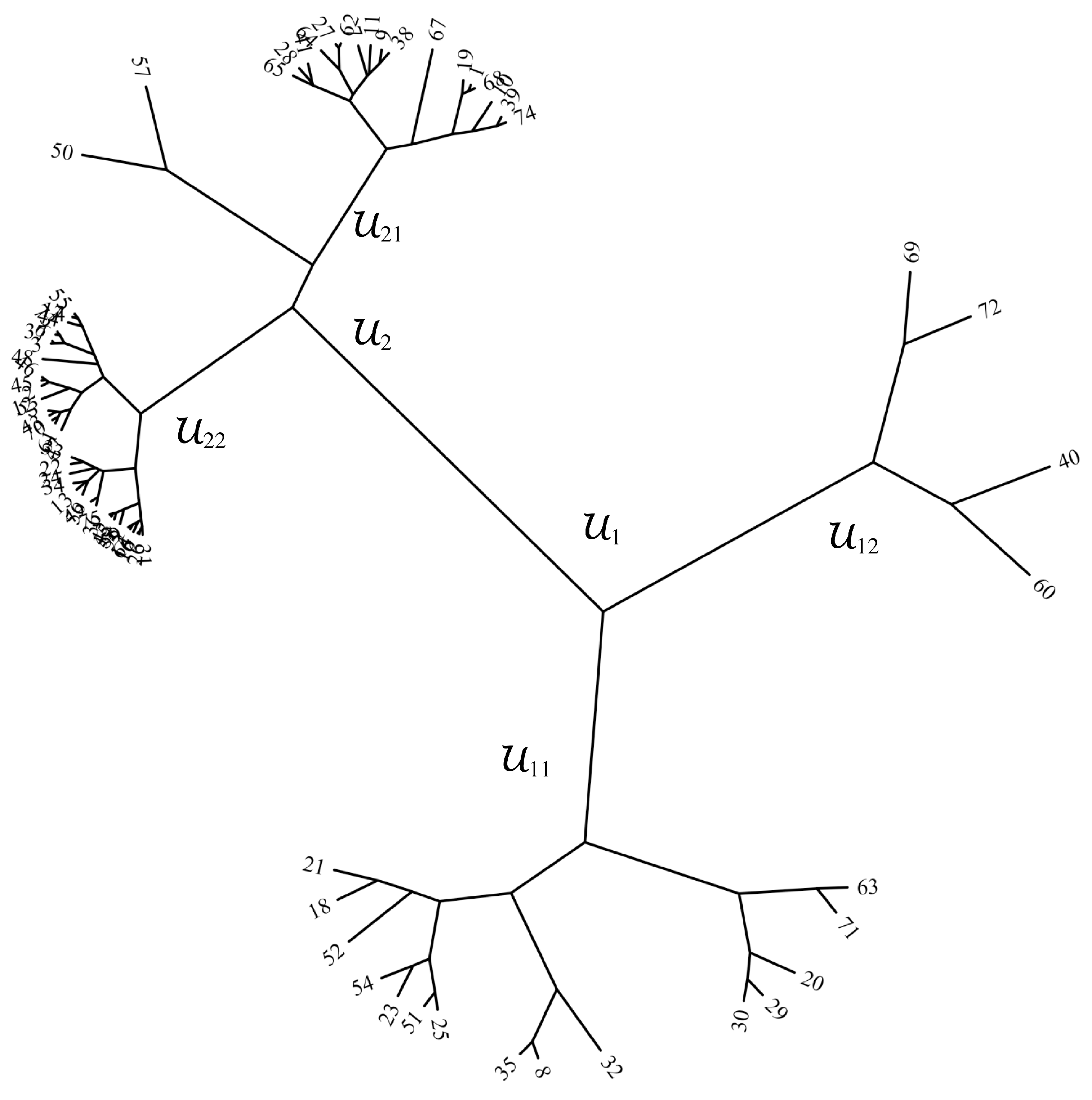
Figure 7.
The continuous wavelet transform (CWT) for Boston (lat: , lon: ) and Christmas Is. (lat: , lon: ) tidal stations. The dashed white lines represent the cones on influence.
Figure 7.
The continuous wavelet transform (CWT) for Boston (lat: , lon: ) and Christmas Is. (lat: , lon: ) tidal stations. The dashed white lines represent the cones on influence.

Figure 8.
The wavelet coherence between Boston (lat: , lon: ) vs. Christmas Is. (lat: , lon: ) and Boston (lat: , lon: ) vs. New York (lat: , lon: ) tidal stations. The dashed white lines represent the cones on influence.
Figure 8.
The wavelet coherence between Boston (lat: , lon: ) vs. Christmas Is. (lat: , lon: ) and Boston (lat: , lon: ) vs. New York (lat: , lon: ) tidal stations. The dashed white lines represent the cones on influence.

Figure 9.
The hierarchical tree resulting from , , with , and calculated based on the CWT.

Figure 10.
The , , and PL approximation for Boston tidal station, yielding .

Figure 11.
Locus of the (a, b) parameters and the polynomial (degree ) fit to , . The size and color of the markers are proportional to the value of the root mean squared error (RMSE) of the PL fit to the MM estimates, , .
Figure 11.
Locus of the (a, b) parameters and the polynomial (degree ) fit to , . The size and color of the markers are proportional to the value of the root mean squared error (RMSE) of the PL fit to the MM estimates, , .

Table 1.
Stations’ labels, names, and percentage of missing data.
| Label | Name | Missing Data (%) | Label | Name | Missing Data (%) | Label | Name | Missing Data (%) |
|---|---|---|---|---|---|---|---|---|
| 1 | Antofagasta | 5.4 | 26 | Granger Bay | 47.1 | 51 | Pensacola | 4.3 |
| 2 | Atlantic City | 3.5 | 27 | Guam | 11.4 | 52 | Petersburg | 0.6 |
| 3 | Balboa | 1.8 | 28 | Kahului Harbor | 0.3 | 53 | Ponta Delgada | 16.7 |
| 4 | Boston | 0.5 | 29 | Kaohsiung | 4.8 | 54 | Port Isabel | 0.4 |
| 5 | Broome | 1.7 | 30 | Keelung | 23.2 | 55 | Portland | 0.9 |
| 6 | Buenaventura | 12.9 | 31 | Knysna | 40.4 | 56 | Prince Rupert | 0.2 |
| 7 | Callao | 4.4 | 32 | Ko Lak | 5.3 | 57 | Pte Des Galets | 23.1 |
| 8 | Charlotte Amalie | 3.9 | 33 | Langkawi | 1.4 | 58 | Puerto Montt | 5.3 |
| 9 | Chichijima | 0 | 34 | Legaspi | 16.9 | 59 | Richard’s Bay | 36.4 |
| 10 | Christmas Is | 6.9 | 35 | Lime Tree Bay | 0.4 | 60 | Rockport | 0.1 |
| 11 | Cocos Is. | 0.9 | 36 | Lobos de Afuera | 14.8 | 61 | Rorvik | 15.2 |
| 12 | Cuxhaven | 0 | 37 | Luderitz | 63.8 | 62 | Saipan | 13.5 |
| 13 | Darwin | 0.2 | 38 | Maisaka | 0.1 | 63 | Salalah | 14.7 |
| 14 | Durban | 39.6 | 39 | Malakal | 1 | 64 | San Juan Puerto Rico | 1 |
| 15 | Dzaoudzi | 65.6 | 40 | Marseille | 31.5 | 65 | Santa Monica | 1.5 |
| 16 | East London | 37.6 | 41 | Mera | 0 | 66 | Simon’s Bay | 41.3 |
| 17 | Eastport | 2.4 | 42 | Mombasa | 30.5 | 67 | Spring Bay | 0.6 |
| 18 | Esperance | 2.5 | 43 | Nain | 50.8 | 68 | Tofino | 2.8 |
| 19 | Fort Denison | 1 | 44 | Napier | 19.4 | 69 | Toyama | 0 |
| 20 | Fort-de-France | 57.5 | 45 | New York | 13.1 | 70 | Vardoe | 1.3 |
| 21 | Fremantle | 0 | 46 | Newport | 0.3 | 71 | Victoria | 0.4 |
| 22 | Funafuti | 1.9 | 47 | Ny-Alesund | 0.3 | 72 | Wakkanai | 0 |
| 23 | Galveston | 2.2 | 48 | Pago Pago | 3.3 | 73 | Walvis Bay | 59 |
| 24 | Gan | 0.2 | 49 | Paita | 10.9 | 74 | Yap | 9 |
| 25 | Grand Isle | 3.1 | 50 | Papeete | 3.3 | 75 | Zanzibar | 5.3 |
Table 2.
Standard tidal constituents.
| Name | Symbol | Period (h) | Speed (/h) |
|---|---|---|---|
| Higher Harmonics | |||
| Shallow water overtides of principal lunar | 6.210300601 | 57.9682084 | |
| Shallow water overtides of principal lunar | 4.140200401 | 86.9523127 | |
| Shallow water terdiurnal | 8.177140247 | 44.0251729 | |
| Shallow water overtides of principal solar | 6 | 60 | |
| Shallow water quarter diurnal | 6.269173724 | 57.4238337 | |
| Shallow water overtides of principal solar | 4 | 90 | |
| Lunar terdiurnal | 8.280400802 | 43.4761563 | |
| Shallow water terdiurnal | 8.38630265 | 42.9271398 | |
| Shallow water eighth diurnal | 3.105150301 | 115.9364166 | |
| Shallow water quarter diurnal | 6.103339275 | 58.9841042 | |
| Semi-Diurnal | |||
| Principal lunar semidiurnal | 12.4206012 | 28.9841042 | |
| Principal solar semidiurnal | 12 | 30 | |
| Larger lunar elliptic semidiurnal | 12.65834751 | 28.4397295 | |
| Larger lunar evectional | 12.62600509 | 28.5125831 | |
| Variational | 12.8717576 | 27.9682084 | |
| Lunar elliptical semidiurnal second-order | 12.90537297 | 27.8953548 | |
| Smaller lunar evectional | 12.22177348 | 29.4556253 | |
| Larger solar elliptic | 12.01644934 | 29.9589333 | |
| Smaller solar elliptic | 11.98359564 | 30.0410667 | |
| Shallow water semidiurnal | 11.60695157 | 31.0158958 | |
| Smaller lunar elliptic semidiurnal | 12.19162085 | 29.5284789 | |
| Lunisolar semidiurnal | 11.96723606 | 30.0821373 | |
| Diurnal | |||
| Lunar diurnal | 23.93447213 | 15.0410686 | |
| Lunar diurnal | 25.81933871 | 13.9430356 | |
| Lunar diurnal | 22.30608083 | 16.1391017 | |
| Solar diurnal | 24 | 15 | |
| Smaller lunar elliptic diurnal | 24.84120241 | 14.4920521 | |
| Smaller lunar elliptic diurnal | 23.09848146 | 15.5854433 | |
| Larger lunar evectional diurnal | 26.72305326 | 13.4715145 | |
| Larger lunar elliptic diurnal | 26.86835 | 13.3986609 | |
| Larger elliptic diurnal | 28.00621204 | 12.8542862 | |
| Solar diurnal | 24.06588766 | 14.9589314 | |
| Long Period | |||
| Lunar monthly | 661.3111655 | 0.5443747 | |
| Solar semiannual | 4383.076325 | 0.0821373 | |
| Solar annual | 8766.15265 | 0.0410686 | |
| Lunisolar synodic fortnightly | 354.3670666 | 1.0158958 | |
| Lunisolar fortnightly | 327.8599387 | 1.0980331 | |
© 2017 by the authors. Licensee MDPI, Basel, Switzerland. This article is an open access article distributed under the terms and conditions of the Creative Commons Attribution (CC BY) license (http://creativecommons.org/licenses/by/4.0/).
Share and Cite
MDPI and ACS Style
M. Lopes, A.; Tenreiro Machado, J.A. Tidal Analysis Using Time–Frequency Signal Processing and Information Clustering. Entropy 2017, 19, 390. https://doi.org/10.3390/e19080390
AMA Style
M. Lopes A, Tenreiro Machado JA. Tidal Analysis Using Time–Frequency Signal Processing and Information Clustering. Entropy. 2017; 19(8):390. https://doi.org/10.3390/e19080390
Chicago/Turabian StyleM. Lopes, Antonio, and Jose A. Tenreiro Machado. 2017. "Tidal Analysis Using Time–Frequency Signal Processing and Information Clustering" Entropy 19, no. 8: 390. https://doi.org/10.3390/e19080390
Note that from the first issue of 2016, this journal uses article numbers instead of page numbers. See further details here.