Intrinsic Losses Based on Information Geometry and Their Applications


College of Mathematics, Sichuan University, Chengdu 610064, China
*
Author to whom correspondence should be addressed.
Entropy 2017, 19(8), 405; https://doi.org/10.3390/e19080405
Submission received: 30 April 2017
/
Revised: 21 July 2017
/
Accepted: 3 August 2017
/
Published: 6 August 2017
(This article belongs to the Special Issue Information Geometry II)
Abstract
:One main interest of information geometry is to study the properties of statistical models that do not depend on the coordinate systems or model parametrization; thus, it may serve as an analytic tool for intrinsic inference in statistics. In this paper, under the framework of Riemannian geometry and dual geometry, we revisit two commonly-used intrinsic losses which are respectively given by the squared Rao distance and the symmetrized Kullback–Leibler divergence (or Jeffreys divergence). For an exponential family endowed with the Fisher metric and -connections, the two loss functions are uniformly described as the energy difference along an -geodesic path, for some . Subsequently, the two intrinsic losses are utilized to develop Bayesian analyses of covariance matrix estimation and range-spread target detection. We provide an intrinsically unbiased covariance estimator, which is verified to be asymptotically efficient in terms of the intrinsic mean square error. The decision rules deduced by the intrinsic Bayesian criterion provide a geometrical justification for the constant false alarm rate detector based on generalized likelihood ratio principle.
1. Introduction
In Bayesian analysis, the choices of a particular loss function and a featured type of priors strongly influence the resulting inference. From the standpoint of purely inference, the final results are typically required to be independent of the way that the model has been parameterized. Thus, in order to produce a Bayes estimator or action which only depends on the model assumed and the data observed, an intrinsic loss and a noninformative (or uninformative) prior are demanded. In an early paper [1], the intrinsic losses are also called the noninformative losses, since they are considered as an analogous determination of the noninformative priors. The reference [1] describes an intrinsic loss as the automated derivation from the sampling distribution without subjective inputs. Whereafter, the entropy and Hellinger losses are suggested there as two appropriate distances between distributions, and their properties are studied especially for exponential families. Some latter works by Barcelona et al. regard the additional requirements as reasonable that the intrinsic losses need be invariant under reduction to sufficient statistics [2]. A symmetric version of Kullback–Leibler (KL) divergence (also named “the intrinsic discrepancy”) as such an intrinsic loss is highly recommended, and has been widely applied to develop intrinsic Bayesian analyses of hypothesis testing [3,4], point estimation [4,5,6,7], and interval estimation [2,4,7].
The invariance criteria achieved by the intrinsic losses are indeed consistent with one main topic of information geometry, which concentrates on excavating the properties of statistical manifolds that are preserved over coordinate system transformations [8]. Under certain regularity conditions, each parametric statistical model possesses a Riemannian manifold structure given by the Fisher metric, with the parametrization identical to a coordinate system [9]. The parameters are merely labels for probability distributions, just as the coordinates for geometric objects. Moreover, the manifold structure supplied by the Fisher metric and -connections are proven to be invariant under transformations of coordinates and reduction by sufficiency [10]. Following this line, a concept is intrinsic if it has a well-defined geometrical meaning. The Riemannian distance in this case—also named the Rao distance [11]—is taken as an intrinsic measure for the dissimilarity between two probability distributions. The reference [12] regards the squared Rao distance between the models labelled by the actual value of the parameter and its estimate as the most natural intrinsic loss, which has been utilized to seek intrinsic Bayes estimators in some concrete univariate examples. In the wider literature, statisticians also apply the Rao distance measure to stimulate the intrinsic study of nonlinear filtering [13], estimation fusion [14,15], and target tracking [16]. Besides, the intrinsic versions of the bias, mean square error (MSE) and Cramér–Rao bound (CRB) are put forward [17,18], which help conduct a systematic analysis for intrinsic estimation theory.
From the above, we can conclude that the Rao distance and the KL divergence are widely accepted as foundation quantities for the intrinsic losses. The former is well-defined on the statistical manifolds with consideration of its usual Riemannian structure, while the later is extremely famous in information theory and is also associated with the canonical divergence in Amari’s dual geometries [9,19]. In this paper, we revisit two intrinsic losses that are given by the squared Rao distance and the symmetric KL divergence (also called the Jeffreys divergence), by integrating them in the framework of information geometry. For the exponential families, they are shown to be uniformly described as the energy difference along an -geodesic path on the statistical manifold, with some . Additionally, the Jeffreys prior—as one of the most popular noninformative priors—corresponds to the Riemannian volume in this setting [20]. The elucidation of their geometrical meanings contributes to deepen our understanding and capabilities in intrinsic Bayesian analysis. Subsequently, we apply these two intrinsic losses to develop Bayesian approaches to covariance matrix estimation and range-spread target detection, which are both hot issues in radar signal processing. The sample covariance matrix (the maximum likelihood estimator (MLE) using a set of zero-mean Gaussian samples) is proven to be intrinsically biased [18]. We provide a Bayesian approach to estimate the scale factor of the sample covariance matrix, which leads to an intrinsically unbiased and asymptotically efficient covariance estimator. The detection of range-spread target is, in essence, a decision problem. Intrinsic analysis supplies a novel way to derive a consistent decision rule under different coordinate systems of measurement. The produced detectors are equivalent to a classical result based on generalized likelihood ratio principle, which will benefit an intuitive interpretation about the geometrical nature of the latter.
In the next section, we review some basic facts about information geometry and exponential family. In Section 3, we present the intrinsic Bayesian approaches to point estimation and hypothesis testing. In Section 4, some applications to covariance matrix estimation and range-spread target detection are studied in detail. Section 5 concludes.
2. The Riemannian Geometry and Dual Geometry of Exponential Family
2.1. The Fisher Metric and the -Connections
Assume a statistical model to describe the probabilistic behavior of a random variable , with the parameter space being an open set of . Under certain regularity conditions, S can be regarded as a differentiable manifold, with being a coordinate system. The manifold S carries the Riemannian structure induced by the Fisher information matrix ,
where signifies the expectation with respect to . In this geometric setting, plays the key role of a metric tensor [11], called the Fisher metric. Then, the infinitesimal squared distance between two closely-spaced distributions and is defined as [21]
For a smooth manifold, the notion of affine connections permits a covariant differential calculus on its tangent bundle. A statistical manifold S possesses a one-parameter family of affine connections related to the Fisher metric, named the -connections (see [9,22]). For an arbitrary real number , the -connection can be given by the Christoffel symbols of the first kind
for . Specially, the 0-connection is exactly the Riemannian (or Levi–Civita) connection with respect to the Fisher metric, and the exponential connection and the mixture connection also have good applications in statistical analysis (e.g., [23,24]).
As detailed in [9], the geometric structure given by the Fisher metric and the -connections obeys the following two invariance principles:
- (1)
- It is invariant under one-to-one reparameterizations.
- (2)
- It is invariant under reduction to sufficient statistics.
2.2. Geometric Structure of Exponential Family
An exponential family is a statistical model S consisting of probability densities of the form
where and , are real-valued functions of , are the so-called natural parameters, and corresponds to the normalization constant. Besides, the functions are generally required to be linearly independent [8]. The exponential families include many common statistical models, such as Gaussian, Poisson, Bernoulli, Gamma, and Dirichlet distributions.
For an exponential family S, let us investigate its geometric structure with respect to the Fisher metric g and -connection . From Equation (3), we can obtain
Note that in information geometry, the differentiation and integration of are customarily assumed to be interchangeable [9]. We can easily verify that an exponential family satisfies this assumption by reference to [25]. Thus from Equations (1) and (4), it is possible to write the components of g as
Further computations by Equation (2) give the expressions for . Especially, we have for .
In essence, the differential geometry with respect to the Fisher metric and the 0-connection coincides with the usual Riemannian geometry. For all exponential families, it is difficult to derive a general theory of their Riemannian geometric structures. Individually, however, the properties of univariate and multivariate Gaussian distributions are well-studied under the framework of Riemannian geometry in [26].
Amari and Nagaoka [9,19] propose the analysis of the geometric structures of statistical models through duality. Typically, an exponential family S has a dually flat structure . That is to say, S is flat with respect to the dual connections and . On the dual flat space , the natural parameters constitute the 1-affine coordinate system, while the -affine coordinate system can be given by the expectation parameters . Furthermore, we can prove that the two potential functions provided by and satisfy
where is the -th entry of the inverse Fisher information matrix , are the 1-affine coordinates of , are the -affine coordinates of , and denotes the KL divergence from p to q.
2.3. -Geodesics
In the presence of an affine connection, geodesics are defined to be curves whose tangent vectors remain parallel if they are transported along it. Specifically, an -geodesic is characterized by the equation
where denotes the derivative with respect to t.
It is well-known in differential geometry that the (locally) shortest curve between two points of the manifold (if it exists) is a 0-geodesic (namely the geodesic in usual Riemannian geometry; e.g., [27]). Usually, a description is used that the 0-geodesic has “constant speed”, since its velocity fields have constant Riemannian norm. Under certain boundary conditions, when , an explicit solution to Equation (8) for univariate or multivariate Gaussian distributions has been derived in [26,28,29]. However, it seems complicated to give out a general closed form of the 0-geodesics for all exponential families.
From the viewpoint of flatness, the manifold S of exponential family is dually flat with respect to . We can know from [19] that any - or 1-geodesic on S is a straight line with respect to the corresponding affine coordinate system. Thus, in terms of the and coordinates, the -geodesics and connecting any can be expressed by
with the parameter . Note that in Equation (9), the velocity fields are constant along t, but and do not have constant speeds.
Example 1 (Univariate Gaussian Distribution).
The probability density of a univariate Gaussian distribution with mean μ and variance can be expressed as
where , and
Further, we can compute the expectation parameters . Figure 1 illustrates the 0- and -geodesics on the manifold of univariate Gaussian distributions.
2.4. The Length and Energy of a Curve
The length of a piecewise smooth curve is defined as
In some occasions, it may be more convenient to work with another related quantity termed the “energy function”, which is given by the integration of the Fisher information along the curve:
Minimizing energy turns out to be equivalent to minimizing length, and both lead to the 0-geodesics on the manifold.
Remark 2.
On a manifold, both the length and energy of a curve do not change under different coordinate systems or model parameterizations, but the latter will depend on the curve parametrization [30].
Now we discuss the lengths and energies of the 0- and -geodesics on the manifold S of exponential family. If there exists a unique 0-geodesic connecting , the length of this 0-geodesic segment equals the well-known Rao distance between p and q [26], written as . From Remark 2, the energy of a curve is meaningless without specifying its parametrization. What we mainly consider in this paper are the 0- and geodesics parameterized by . Since the 0-geodesics have constant speed, it means that the integrands in Equations (10) and (11) are constant over t. Thus, given a 0-geodesic connecting p and q, its length and energy have the following relationship [30]:
The -geodesics on S have explicit expressions, shown in Equation (9). Furthermore, the theorem given below describes their energy functions.
Theorem 3.
The energies of the -geodesics given in Equation (9) are equal to the Jeffreys divergence between p and q.
Proof.
As an example, on the manifold of univariate Gaussian distributions, Figure 2 shows the energy differences along the -geodesics parameterized by , for . We have known that the 0-geodesic path follows the minimum energy variation, which is also demonstrated in Figure 2. Below is a straightforward corollary of Theorem 3.
Corollary 4.
If p and q belong to the same exponential family, then .
3. Intrinsic Bayesian Analysis
3.1. Two Intrinsic Losses
Suppose that the observed data are generated by , for some . Let be the actual (unknown) value of the parameter, and be a given value which may represent an estimator or a hypothesis. For the problems of statistical inference, we define a loss function , aiming at measuring the consequences of estimating by in statistical estimation [5] or judging the compatibility of with the observations in hypothesis testing [3].
Many conventional loss functions (such as the squared error loss, the zero-one loss) are defined to compare and in the parameter space, while an intrinsic loss function tends to directly measure the dissimilarity between and . As customary, the intrinsic losses are required to be invariant under one-to-one transformations of either or (e.g. [2,5]). Let form an n-dimensional manifold. From the viewpoint of information geometry, the aforementioned criteria are satisfied if a loss function has a well-defined geometrical meaning. Therefore, based on the contents of Section 2.4, we will consider the following two intrinsic losses:
- (i)
- Intrinsic loss based on the squared Rao distance (hereafter referred to as the Rao loss):which stands for the energy difference along a 0-geodesic connecting and on S and parameterized by .
- (ii)
- Intrinsic loss based on the Jeffreys divergence (hereafter referred to as the Jeffreys loss):which stands for the energy difference along a - or 1-geodesic connecting and on S and parameterized by if S is an exponential family.
Since the Jeffreys divergence is a symmetrized KL divergence, it has all the properties of a metric as defined in topology except the triangle inequality property, and is thus not termed a distance. In recent years, this quantity has sometimes been used for model selection [31,32]. There exists another symmetrized version of KL divergence proposed in [2,5] for intrinsic analysis, which takes a minimum over and thus copes better with the case when and have nested supports. Even so, we prefer to adopt the Jeffreys loss in this paper since it has a better-understood geometrical interpretation.
3.2. Priors
Apart from the loss function, an appropriate choice of the prior distribution plays an equally strong role for Bayesian analysis. A particular type of priors have been developed to cope with noninformative settings, where the term “noninformative” expresses that a prior distribution in the Bayes theory is expected to have minimal effect on the posterior inference [5]. A common noninformative prior for the Bayesian paradigm is the Jeffreys prior, which is proportional to the Riemannian volume corresponding to the Fisher metric [20]. As we have learned from the geometric theory, this is an intrinsic concept and is thus not dependent on the model parametrizations.
In many early works, the Jeffreys priors are not recommended for multiparameter cases. Bernardo [33] has initiated the reference priors in Bayesian inference (also known as objective Bayesian inference), which is widely accepted for various multiparameter Bayesian problems. However, in most multidimensional occasions, the analytical evaluations related to an inference prior appear to be quite cumbersome. Thus, some numerical algorithms are designed to do the computations in objective Bayesian inference (e.g., [34,35]), which seems unfavorable for the theoretical derivations of this paper. Additionally, in Section 4, the applications of Jeffreys priors yield an appropriate scale of the eigenvalues of sample covariance matrix, and also reproduce the classic constant false alarm ratio (CFAR) detector in radar detection theory. Hence, we believe that the Jeffreys prior may give a different consequence in intrinsic Bayesian analysis.
3.3. Intrinsic Bayesian Analysis
Let be the posterior distribution with respect to the prior . From a Bayesian viewpoint, the corresponding posterior expected loss is
Considering the invariance criteria, we take the loss function as or and use the Jeffreys prior . This paper will discuss two aspects of intrinsic Bayesian inference: point estimation and hypothesis testing.
As formulated in [3], a hypothesis testing problem is to decide how the observed data are compatible with the null hypothesis. Specifically, when the null hypothesis contains only one value , an intrinsic Bayesian approach to this hypothesis test is based on the positive statistic , which suggests to reject the null hypothesis if with some threshold ; for the composed null hypothesis case, it is suggested to take as the test statistic, where denotes the null parameter space.
When we come to deal with a point estimation problem, the Bayes estimator of is obtained by minimizing the posterior expected loss function:
from which the obtained estimator is invariant under invertible transformations of either or . Besides, the property of can be further analyzed using the intrinsic estimation theory.
Before finishing this subsection, it is convenient to introduce some basic concepts of intrinsic estimation theory. Fix a and let be the tangent space at . Associated with a considered connection ∇, the corresponding geodesic curve with starting point and initial direction is denoted by . Such a curve exists when belongs to a small neighborhood of the origin at . In this case, the exponential map is defined as . Given an estimator , the estimator vector field is induced on S through the inverse of exponential map: . Further, the bias vector field is defined as
If for any , the estimator is called intrinsically unbiased. Obviously, these definitions above are dependent on the specific choice of ∇ [18]. When a flat connection is considered, an estimator will be intrinsically unbiased if and only if it is unbiased under the corresponding affine coordinate system. Generally speaking, however, the notion of intrinsic unbiasedness is widely acknowledged only in the Riemannian case (namely, when ∇ is the Riemannian connection). Thus, in this paper, when we say that an estimator is intrinsically unbiased, we mean that this is true with regard to the 0-connection. The intrinsic MSE is defined by the mean square of the Rao distance
where, in the Bayesian sense, denotes the expectation taken over both and . An intrinsic version of the CRB gives a lower bound on the intrinsic MSE performance of any intrinsically unbiased or biased estimator. The relevant developments can be found in [17,18,36].
4. Applications
4.1. Covariance Estimation
Let be random samples of size n from a zero-mean p-variate Gaussian distribution with unknown covariance matrix . Consider the Jeffreys prior distribution for ([37], p. 426), . A sufficient statistic is provided by
which is recognized as the sample covariance matrix of the data set [38]. Assume that ; then, is positive definite with probability one. Thus, the corresponding posterior distribution based on the Jeffreys prior is easily found to be
which follows an inverse Wishart distribution with n degrees of freedom and scale matrix .
Now we restrict to consider a family of covariance estimators having the form , which contain the MLE . The Rao distance between and is [39]
while the Jeffreys divergence is [40]
Taking the intrinsic losses into account, we can obtain an intrinsic estimator by minimization of the posterior expected Rao loss function:
where signifies the expectation with respect to . By Equation (15), we have
where denote the p eigenvalues of the matrix . In fact, it proves quite difficult to directly solve the conditional expectation in Equation (16) as a closed form. However, if we let , it is easy to show that the objective function in Equation (16) is a strictly convex function with respect to c. Thus, we can resort to the Lagrange equation to seek the minimum point. Write the posterior expected Rao loss function as
Then, let
By Leibniz’s rule [41], we can interchange the integral and differential operators, obtaining
Since , . Combining with the fact that , we can calculate the conditional expectation in Equation (17) by the law of log-determinant of a Wishart matrix [42]:
where is the well-known digamma function defined as . Thus, from Equation (17), the intrinsic covariance estimator based on the Rao loss is , with
Alternatively, if we consider the Jeffreys loss function , then
It is easy to calculate that , and when ,
Therefore, the intrinsic covariance estimator based on the Jeffreys loss is , with
In Table 1, the scale factors and are evaluated for various values of n and .
We now come to examine the bias and efficiency of these two intrinsic estimators.
Proposition 5.
Let with , then , where m is a constant decided by , and v.
Proof.
For a unitary matrix , the random matrix follows the same distribution with . Thus,
Recall the important fact that , where and are two nonsingular matrices. Thus, a further step yields
Note that the equality above holds for an arbitrary unitary matrix ; then, we can conclude that must be a scalar multiple of the identity matrix. ☐
Theorem 6.
The covariance estimator given by Equation (18) is intrinsically unbiased.
Proof.
For a p-dimensional positive-definite matrix , the inverse of the exponential map defined on the manifold of positive definite matrices is given by [43]
Thus, we have
Generally, it is difficult to directly solve the expectation of the logarithm of a Wishart matrix. However, since , by Proposition 5, the expectation in Equation (19) has this form
with a certain constant m. In addition, since
we can obtain
Substituting Equations (18), (20) and (21) into Equation (19), we have , which indicates that the covariance estimator is intrinsically unbiased. ☐
Given a real number , the posterior expected Rao loss of can be computed by
Using Proposition 5 again, we know that the right-hand side of the second equality above is constant on the sample space. Thus, the posterior expected Rao losses of , and are equal to their Bayes risks under Rao loss that average the Rao loss functions over both sample space and parameter space. Similar consequences can be deduced for the posterior expected Jeffreys losses of , and their Bayes risks under Jeffreys loss. It is still difficult to seek an explicit expression for the posterior expected Rao loss. Hence, a Monte Carlo simulation is used with 1000 trials to calculate the Bayes risks under Rao loss. The comparisons are illustrated in Figure 3.
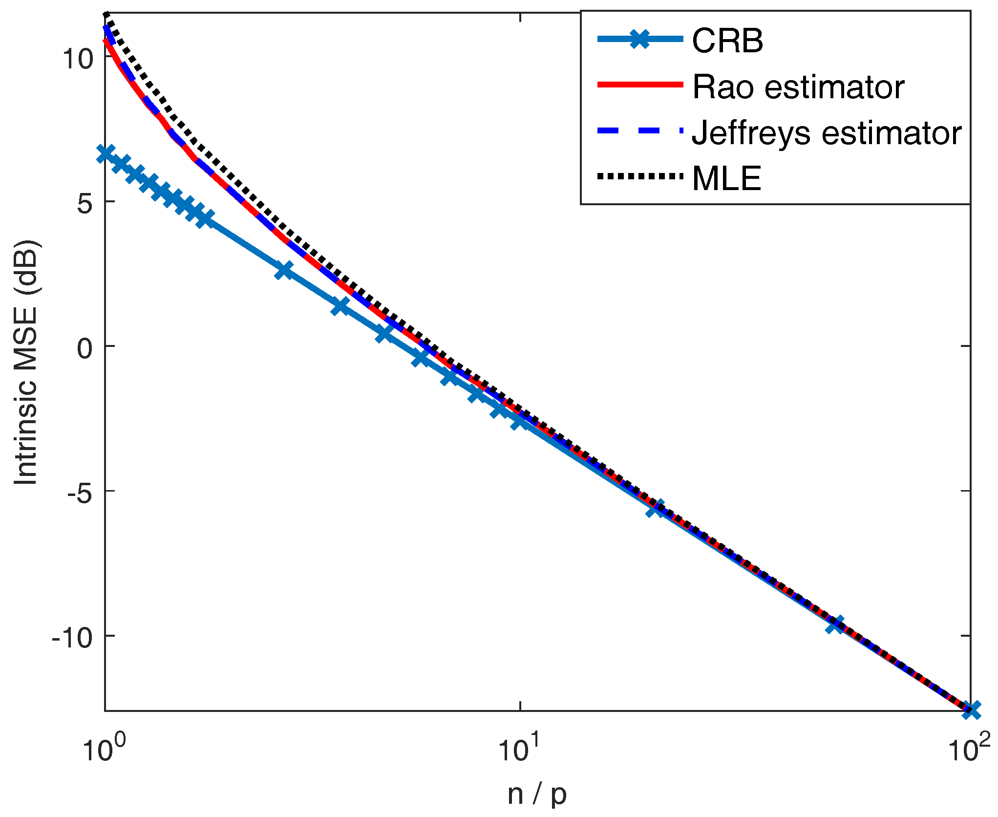
In Figure 4, we compare the intrinsic MSEs (see Equation (14)) of the considered estimators with an intrinsic version of the CRB given in ([18], Theorem 4), which serves as a lower bound for any intrinsically unbiased covariance estimator. In fact, for our case, the intrinsic MSEs of and are equal to their Bayes risks under Rao loss. Recalling that the MLE is not intrinsically unbiased but always asymptotically efficient [18], we can conclude that the Bayes estimator under Rao loss is intrinsically unbiased and also asymptotically efficient. This property is also demonstrated in Figure 4.
4.2. Range-Spread Target Detection
The target detection in the background of Gaussian noise is a basic problem in radar signal processing. Suppose that an unknown target is spatially distributed across H range cells. Data collected from these H cells—called the primary data—consist of the possible target echoes plus Gaussian noises. As in [44], we assume that a set of secondary data coming from K cells arranged around the target are available, which serve as training samples for noise covariance estimation. Here the homogeneous noise environment is considered, which means that the secondary data are free of signal components and share the same distribution as the noise-only part of the primary data. Therefore, the considered detection problem can be formulated as [44]
where denote the N-dimensional unknown signal vectors, and , are independent and identically distributed Gaussian noises with mean zero and unknown covariance matrix . For the brevity of notation, let us introduce the matrix forms
Denote and , then the matrix of measurements is Gaussian distributed with mean and covariance . In the absence of target, we have under the null hypothesis. Therefore, the Rao distance between the assumed model and the null model is [45]
We shall adopt again the Jeffreys prior distribution for parameters [35]:
The joint density for is proportional to
where . Thus, the corresponding posterior distribution satisfies
Since , we can conclude that
Therefore, the posterior expected Rao loss of determining the null hypothesis is derived as follows:
Hence, the decision rule for the compatibility of the null hypothesis with the observed data can be given as
where the threshold is chosen by the required false alarm probability. In fact, this result reproduces the two-step generalized likelihood ratio test [46] or Wald test [47], which is verified to have CFAR property [46].
Besides, since in this case,
we can derive an equivalent decision rule using the Jeffreys loss.
Finally, as a conclusion of this section, we will conduct a discussion about the relationship between the geometric invariance principle and the CFAR property. If we transform the random variables to without altering the structures of statistical model and testing problem, it is equivalent to derive a transformation on the parameter space . Let a decision statistic be an intrinsic concept in the geometrical meaning. Thus, this statistic is invariant by changing to , which indicates that it maintains a CFAR behavior over an orbit of the parameter space.
5. Conclusions
In this paper, the Rao loss and Jeffreys loss—which are, respectively, based on the squared Rao distance and the Jeffreys divergence—are uniformly considered in the framework of information geometry. We have elucidated their geometrical meaning based on some results of Riemannian geometry and dualistic geometry. In particular, on the manifold of an exponential family, the Rao loss and Jeffreys loss are essentially the energy differences along -geodesic paths parameterized by , for . Based on this, they certainly enjoy the invariance properties under the one-to-one transformations of random variables and model parameters. Subsequently, these two intrinsic loss functions are unitized to develop intrinsic Bayesian analysis of covariance estimation and range-spread target detection. We use the intrinsic losses to derive the scale factor of sample covariance matrix, which leads to an intrinsically unbiased and asymptomatically efficient covariance estimator. On the other hand, the detectors provided by the posterior expected intrinsic losses have been proven to coincide with the classic CFAR detector in radar detection theory. In this respect, it seems to be a novel but promising approach to derive a detector having CFAR property though intrinsic analysis.
Acknowledgments
This work was supported in part by the National Natural Science Foundation of China under grant 61374027, the Program for Changjiang Scholars and Innovative Research Team in University under grant IRT_16R53 from the Chinese Education Ministry, and the Specialized Research Fund for the Doctoral Program of Higher Education under grant 20130181110042.
Author Contributions
Yao Rong and Mengjiao Tang put forward the original ideas and conducted the research; Jie Zhou raised the research question, reviewed this paper and provided improvement suggestions. All authors have read and approved the final manuscript.
Conflicts of Interest
The authors declare no conflict of interest.
References
- Robert, C.P. Intrinsic losses. Theor. Decis. 1996, 40, 191–214. [Google Scholar] [CrossRef]
- Bernardo, J.M. Intrinsic credible regions: An objective Bayesian approach to interval estimation. Test 2005, 14, 317–384. [Google Scholar] [CrossRef]
- Bernardo, J.M. Nested hypothesis testing: The Bayesian reference criterion. In Bayesian Statistics 6; Bernardo, J.M., Berger, J.O., Dawid, A.P., Smith, A.F.M., Eds.; Oxford University Press: Oxford, UK, 1999; pp. 101–130. [Google Scholar]
- Bernardo, J.M. Integrated objective Bayesian estimation and hypothesis testing. In Bayesian Statistics 9; Bernardo, J.M., Bayarri, M.J., Berger, J.O., Dawid, A.P., Heckerman, D., Eds.; Oxford University Press: Oxford, UK, 2010; pp. 1–68. [Google Scholar]
- Bernardo, J.M.; Juárez, M. Intrinsic estimation. In Bayesian Statistics 7; Bernardo, J.M., Bayarri, M.J., Berger, J.O., Dawid, A.P., Heckerman, D., Smith, A.F.M., West, M., Eds.; Oxford University Press: Oxford, UK, 2003; pp. 465–476. [Google Scholar]
- Bernardo, J.M. Intrinsic point estimation of the normal variance. In Bayesian Statistics and Its Applications; Upadhyay, S.K., Singhand, U., Dey, D.K., Eds.; Anamaya Publication: New Delhi, India, 2006; pp. 110–121. [Google Scholar]
- Bernardo, J.M.; Bernardo, J.M. Objective Bayesian point and region estimation in location-scale models. Stat. Oper. Res. Trans. 2007, 31, 3–44. [Google Scholar]
- Calin, O.; Udrişte, C. Geometric Modeling in Probability and Statistics; Springer: Basel, Switzerland, 2014. [Google Scholar]
- Amari, S.I.; Nagaoka, H. Methods of Information Geometry; American Mathematical Society: Providence, RI, USA, 2000. [Google Scholar]
- Čencov, N.N. Statistical Decision Rules and Optimal Inference; Ametrican Mathematical Society: Providence, RI, USA, 1982. [Google Scholar]
- Rao, C.R. Information and accuracy attainable in the estimation of statistical parameters. Bull. Calcutta Math. Soc. 1945, 37, 81–91. [Google Scholar]
- García, G.; Oller, J.M. What does intrinsic mean in statistical estimation? Stat. Oper. Res. Trans. 2006, 30, 125–170. [Google Scholar]
- Darling, R.W.R. Geometrically intrinsic nonlinear recursive filters II: Foundations. Available online: https://arxiv.org/ftp/math/papers/9809/9809029.pdf (accessed on 4 August 2017).
- Ilea, I.; Bombrun, L.; Terebes, R.; Borda, M.; Germain, C. An M-estimator for robust centroid estimation on the manifold of covariance matrices. IEEE Signal Process. Lett. 2016, 23, 1255–1259. [Google Scholar] [CrossRef]
- Tang, M.; Rong, Y.; Zhou, J. Information-geometric methods for distributed multi-sensor estimation fusion. In Proceedings of the 19th International Conference on Information Fusion, Heidelberg, Germany, 5–8 July 2016; pp. 1585–1592. [Google Scholar]
- Cheng, Y.; Wang, X.; Morelande, M.; Moran, B. Information geometry of target tracking sensor network. Inf. Fusion 2013, 14, 311–326. [Google Scholar] [CrossRef]
- Oller, J.M.; Corcuera, J.M. Intrinsic analysis of statistical estimation. Ann. Stat. 1995, 23, 1562–1581. [Google Scholar] [CrossRef]
- Smith, S.T. Covariance, subspace, and intrinsic Cramér-Rao bounds. IEEE Trans. Signal Process. 2005, 53, 1610–1630. [Google Scholar] [CrossRef]
- Amari, S.I. Information Geometry and Its Applications; Springer: Tokyo, Japan, 2016. [Google Scholar]
- Jeffreys, H. An invariant form for the prior probability in estimation problems. Proc. R. Soc. Lond. A Math. Phys. Sci. 1946, 186, 453–461. [Google Scholar] [CrossRef] [PubMed]
- Amari, S.I. Information geometry on hierarchy of probability distributions. IEEE Trans. Inf. Theory 2001, 47, 1701–1711. [Google Scholar] [CrossRef]
- Amari, S.I. Differential-Geometrical Methods in Statistics; Vol. 28, Lecture Notes in Statistics; Springer: New York, NY, USA, 1985. [Google Scholar]
- Amari, S.I. Information geometry of the EM and em algorithms for neural networks. Neural Netw. 1995, 8, 1379–1408. [Google Scholar] [CrossRef]
- Amari, S.I. Information geometry of statistical inference–an overview. In Proceedings of the IEEE Information Theory Workshop, Bangalore, India, 25 October 2002; pp. 86–89. [Google Scholar]
- Ay, N.; Jost, J.; Vân Lê, H.; Schwachhöfer, L. Information geometry and sufficient statistics. Probab. Theory Related Fields 2015, 162, 327–364. [Google Scholar] [CrossRef]
- Skovgaard, L.T. A Riemannian geometry of the multivariate normal model. Scand. J. Stat. 1984, 11, 211–223. [Google Scholar]
- Postnikov, M.M. Geometry VI: Riemannian Geometry; Vol. 91, Encyclopaedia of Mathematical Sciences; Springer: Berlin/Heidelberg, Germany, 2001. [Google Scholar]
- Calvo, M.; Oller, J.M. An explicit solution of information geodesic equations for the multivariate normal model. Stat. Decis. 1991, 9, 119–138. [Google Scholar] [CrossRef]
- Imai, T.; Takaesu, A.; Wakayama, M. Remarks on geodesics for multivariate normal models. J. Math. Industry 2011, 3, 125–130. [Google Scholar]
- do Carmo, M.P. Riemannian Geometry; Birkhäuser: Boston, MA, USA, 1992. [Google Scholar]
- Magnant, C.; Grivel, E.; Giremus, A.; Joseph, B.; Ratton, L. Jeffrey’s divergence for state-space model comparison. Signal Process. 2015, 114, 61–74. [Google Scholar] [CrossRef]
- Legrand, L.; Grivel, E. Evaluating dissimilarities between two moving-average models: A comparative study between Jeffrey’s divergence and Rao distance. In Proceedings of the 24th European Signal Processing Conference, Budapest, Hungary, 29 August–2 September 2016; pp. 205–209. [Google Scholar]
- Bernardo, J.M. Reference posterior distributions for Bayesian inference. J. R. Stat. Soc. Series B Stat. Methodol. 1979, 41, 113–147. [Google Scholar]
- Yang, R.; Berger, J.O. Estimation of a covariance matrix using the reference prior. Ann. Stat. 1994, 22, 1195–1211. [Google Scholar] [CrossRef]
- Sun, D.; Berger, J.O. Objective Bayesian analysis for the multivariate normal model. Proceedings of Valencia / ISBA 8th World Meeting on Bayesian Statistics, Alicante, Spain, 1–6 June 2006; pp. 525–547. [Google Scholar]
- Barrau, A.; Bonnabel, S. A note on the intrinsic Cramer-Rao bound. In Geometric Science of Information; Springer: Berlin/Heidelberg, Germany, 2013; pp. 377–386. [Google Scholar]
- Box, G.E.; Tiao, G.C. Bayesian Inference in Statistical Analysis; Wiley: New York, NY, USA, 1992. [Google Scholar]
- Guerci, J.R. Space-Time Adaptive Processing for Radar; Artech House: Norwood, MA, USA, 2003. [Google Scholar]
- Costa, S.I.; Santos, S.A.; Strapasson, J.E. Fisher information distance: A geometrical reading. Discrete Appl. Math. 2015, 197, 59–69. [Google Scholar] [CrossRef]
- Contreras-Reyes, J.E.; Arellano-Valle, R.B. Kullback–Leibler divergence measure for multivariate skew-normal distributions. Entropy 2012, 14, 1606–1626. [Google Scholar] [CrossRef]
- Protter, M.H.; Morrey, C.B., Jr. Intermediate Calculus; Springer: New York, NY, USA, 1985. [Google Scholar]
- Bishop, C.M. Pattern Recognition and Machine Learning; Springer: New York, NY, USA, 2006. [Google Scholar]
- Moakher, M. A differential geometric approach to the geometric mean of symmetric positive-definite matrices. SIAM J. Matrix Anal. Appl. 2005, 26, 735–747. [Google Scholar] [CrossRef]
- Kelly, E.J. An adaptive detection algorithm. IEEE Trans. Aerosp. Electron. Syst. 1986, 22, 115–127. [Google Scholar] [CrossRef]
- Atkinson, C.; Mitchell, A.F. Rao’s distance measure. Sankhya 1981, 43, 345–365. [Google Scholar]
- Conte, E.; De Maio, A.; Galdi, C. CFAR detection of multidimensional signals: An invariant approach. IEEE Trans. Signal Process. 2003, 51, 142–151. [Google Scholar] [CrossRef]
- Liu, W.; Xie, W.; Wang, Y. Rao and Wald tests for distributed targets detection with unknown signal steering. IEEE Signal Process. Lett. 2013, 20, 1086–1089. [Google Scholar]
Figure 1.
The 0- and -geodesics on the manifold of univariate Gaussian distributions with given endpoints and , under (a) the 1-affine coordinate system and (b) the -affine coordinate system .
Figure 1.
The 0- and -geodesics on the manifold of univariate Gaussian distributions with given endpoints and , under (a) the 1-affine coordinate system and (b) the -affine coordinate system .
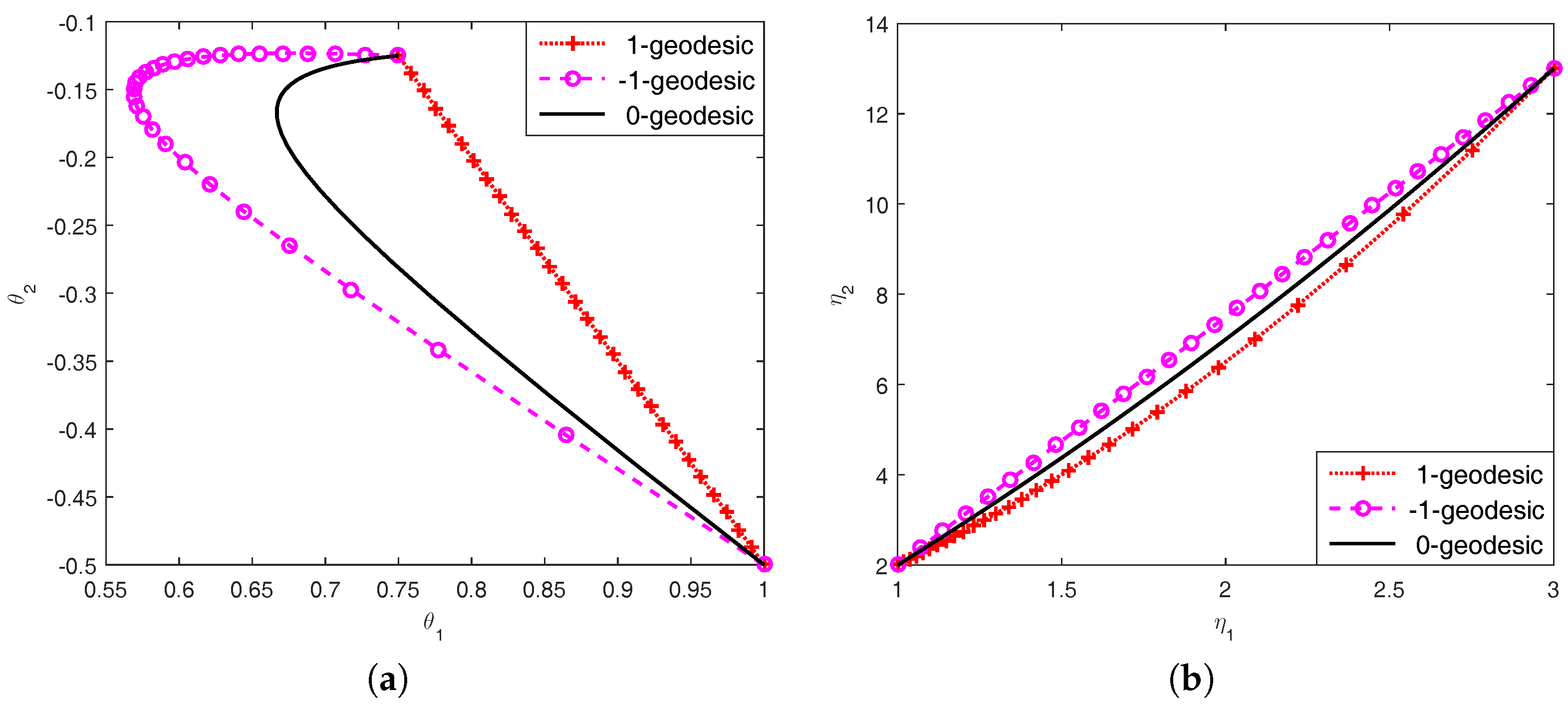
Figure 2.
The energy differences along the 0- and -geodesics parameterized by [0, 1] on the manifold of univariate Gaussian distributions, with start point and end point .
Figure 2.
The energy differences along the 0- and -geodesics parameterized by [0, 1] on the manifold of univariate Gaussian distributions, with start point and end point .
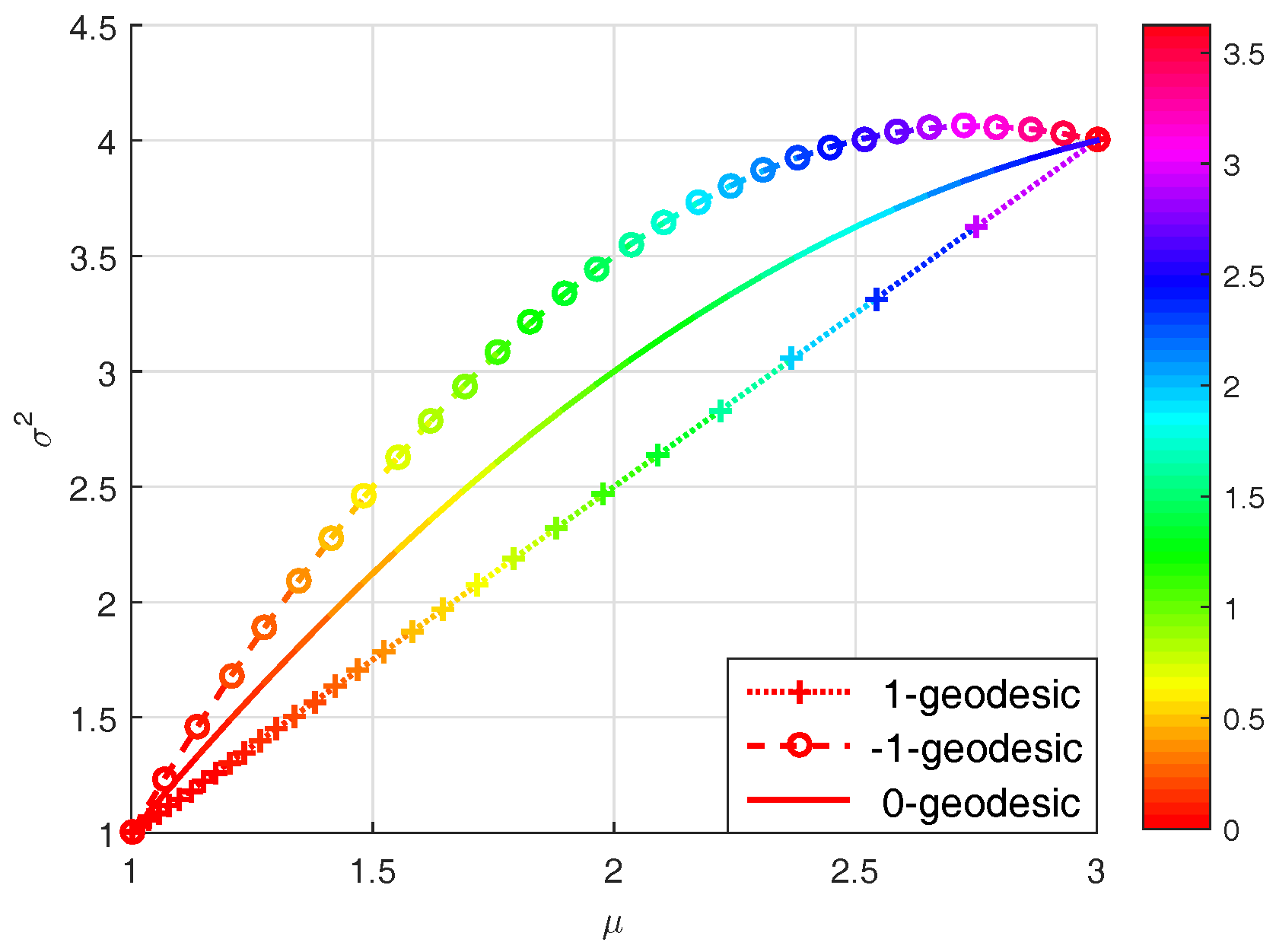
Figure 3.
Comparisons of Bayes risks among (solid line), (dashed line), and (dotted line) for under (a) Rao loss and (b) Jeffreys loss.
Figure 3.
Comparisons of Bayes risks among (solid line), (dashed line), and (dotted line) for under (a) Rao loss and (b) Jeffreys loss.
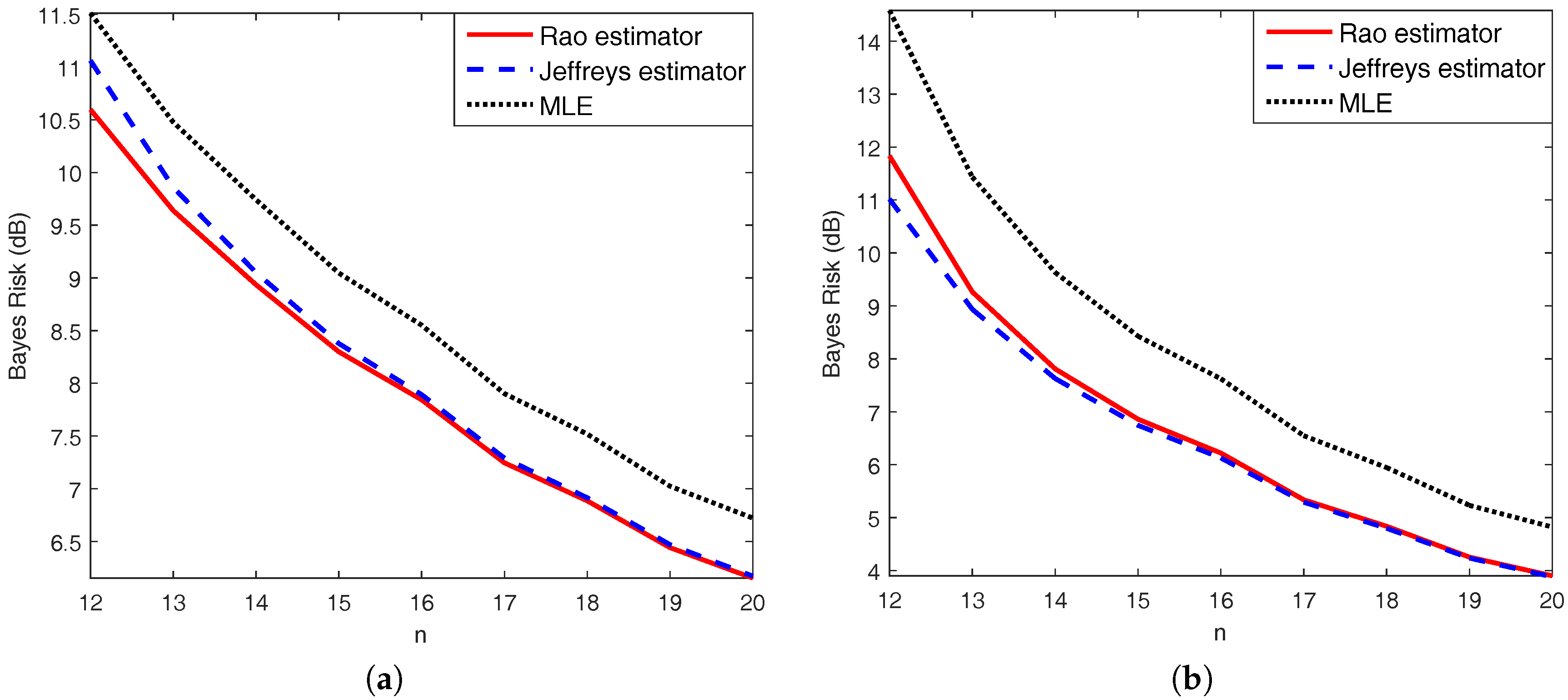
Figure 4.
The intrinsic MSEs of (solid line), (dashed line), and are compared with an intrinsic version of Cramér–Rao bound (CRB) (marked line) for .
Figure 4.
The intrinsic MSEs of (solid line), (dashed line), and are compared with an intrinsic version of Cramér–Rao bound (CRB) (marked line) for .


Table 1.
The scale factors of sample covariance matrix for some values of n and .
| n | n | ||||
|---|---|---|---|---|---|
| 12 | 50 | ||||
| 13 | 100 | ||||
| 14 | 200 | ||||
| 16 | 500 | ||||
| 18 | |||||
| 20 |
© 2017 by the authors. Licensee MDPI, Basel, Switzerland. This article is an open access article distributed under the terms and conditions of the Creative Commons Attribution (CC BY) license (http://creativecommons.org/licenses/by/4.0/).
Share and Cite
MDPI and ACS Style
Rong, Y.; Tang, M.; Zhou, J. Intrinsic Losses Based on Information Geometry and Their Applications. Entropy 2017, 19, 405. https://doi.org/10.3390/e19080405
AMA Style
Rong Y, Tang M, Zhou J. Intrinsic Losses Based on Information Geometry and Their Applications. Entropy. 2017; 19(8):405. https://doi.org/10.3390/e19080405
Chicago/Turabian StyleRong, Yao, Mengjiao Tang, and Jie Zhou. 2017. "Intrinsic Losses Based on Information Geometry and Their Applications" Entropy 19, no. 8: 405. https://doi.org/10.3390/e19080405
Note that from the first issue of 2016, this journal uses article numbers instead of page numbers. See further details here.