Statistical Process Control for Unimodal Distribution Based on Maximum Entropy Distribution Approximation

1
School of Management, Shanghai University, Shanghai 200444, China
2
College of Economics & Management, China Jiliang University, Hangzhou 310018, China
3
School of Management, Shenzhen Polytechnic, Shenzhen 518055, China
*
Author to whom correspondence should be addressed.
Entropy 2017, 19(8), 406; https://doi.org/10.3390/e19080406
Submission received: 21 June 2017
/
Revised: 18 July 2017
/
Accepted: 4 August 2017
/
Published: 7 August 2017
(This article belongs to the Special Issue Maximum Entropy and Bayesian Methods)
Abstract
:In statistical process control, the control chart utilizing the idea of maximum entropy distribution density level sets has been proven to perform well for monitoring the quantity with multimodal distribution. However, it is too complicated to implement for the quantity with unimodal distribution. This article proposes a simplified method based on maximum entropy for the control chart design when the quantity being monitored is unimodal distribution. First, we use the maximum entropy distribution to approximate the unknown distribution of the monitored quantity. Then we directly take the value of the quantity as the monitoring statistic. Finally, the Lebesgue measure is applied to estimate the acceptance regions and the one with minimum volume is chosen as the optimal in-control region of the monitored quantity. The results from two cases show that the proposed method in this article has a higher detection capability than the conventional control chart techniques when the monitored quantity is asymmetric unimodal distribution.
1. Introduction
Statistical Process Control (SPC), based on the control chart and other monitoring methods, has been widely used in manufacturing, service, and industrial practices (see [1]). The conventional Shewhart chart is very popular for monitoring univariate quantity. During the last several decades, the control chart for the mean has been expanded to the well-known Hotelling’s chart, multivariate cumulative sum (CUSUM) chart and exponentially weighted moving average (EWMA) chart (see [2,3]). The Bayesian control chart is also proposed to monitor multivariate quantities (see [4,5]). For these control charts, the basic idea is to establish a probability distribution for the monitored quantity at first that can describe its randomness. Actually, this distribution always remains unknown in most practical situations. Then, test the newly monitored sample against the distribution of the monitored quantity. If the newly monitored sample has an obvious difference from the distribution of the monitored quantity, the process can be decided as out-of control. Otherwise, the process is considered as in-control when the newly monitored sample is similar to the distribution of the monitored quantity (see [6]. For most practical situations, in order to implement SPC easily for practitioners, many conventional SPC techniques take the sample distribution as Normal distribution when the monitored quantity is a continuous variable, e.g., the Shewhart control chart technique, and take the monitored quantity as Poisson or Binomial distribution when it is a discrete variable, e.g., in most situations of sampling inspection in quality control. However, when the quantity being monitored in practical situations is not of the above cases, e.g., for small samples, multivariable and/or auto correlated data (see [7,8]), the performances of the conventional SPC techniques tend to be significantly diminished. Because the control limits are inaccurate, the true Type I error which is called false alarm probability will have a large discrepancy comparing to the designated false alarm probability, as well as for the Type II error which is called miss-detection probability in SPC. To provide sufficiently flexible control methods for more complicated problems, many nonparametric control charts have been proposed in recent researches (see [9]).
The entropy-based techniques have been formalized to detect the randomness of variables. Acharya et al. have discussed the various entropies applied on automated diagnosis of epilepsy using the electroencephalogram (EEG) signal comprehensively (see [10]). For EEG signal monitoring, there are several entropy features extracted from the EEG signal, and it has found many advantages in applying these entropy features, such as separating the useful signal from redundant information, improving the accuracy for epilepsy diagnosis, etc (see [10,11]). In EEG signal diagnosis, the entropy features are calculated as a numerical measure for the chaos of the signal. The entropy-based techniques are also used to detect the shifts of monitored quantities in SPC. Comparing to the EEG signal diagnosis, the entropy is mainly used to determine the probability distributions of monitored quantities. Information-Theoretic Process Control (ITPC) is the signal charting procedures for monitoring the quantity without a need to make distribution assumption (see [12]). In ITPC, Maximum Entropy (ME) distribution is proposed to approximate the distribution for the monitored quantity. Based on the maximum entropy principle, the ME distribution is estimated by maximizing the Shannon entropy subjected to the specified constraints (see [13]). Then, the ITPC method takes the Kullback–Leibler (KL) divergence between the ME distribution and the sample distribution as the monitoring statistic. When the KL divergence is larger than the threshold value, the signalling will be generated to mind that the sample is out-of-control. However, for the case of small sample size, the KL divergence might not perform well (see [6]). Furthermore, when the distribution of the quantity being monitored is multimodal, the in-control region might not be continuous.
Aiming to tackle the weakness of the ITPC method, Das and Zhou (see [6]) have applied the Maximum Entropy Level Set to design the control chart, which is called the MELS chart. Like the ITPC method, it also uses the ME distribution to fit the distribution of the monitored quantity. However, instead of using the KL divergence as the final monitoring statistic, it proposes a new principle to find the optimal in-control region which is more convenient to use and works well for the small size sample. Generally, it takes the function of quantity as the monitoring statistic, with the Type I error ; the optimal in-control region is as
where h denotes the threshold value in the MELS chart. is a polynomial of X and it is expressed as the exponential part of the ME distribution function (see Section 2). For the newly monitored sample, when , it belongs to the out-of-control region. Otherwise, the newly monitored sample is in-control. The main principle in MELS is: given the Type I error , it selects the density level set with the minimum volumes to be the optimal in-control region. The MELS chart has been proven to perform better than the ITPC method for the multimodal distributions such as mixture Normal distributions. Because of the multimodal distributions, the acceptance region of X is probably not a continuous set. Take the multimodal distribution of from Das and Zhou’s (see [6]) research as an example. With , when h was found to be 2.894, then X belonging to the acceptance region is . By using , it can make the in-control region expression one continuous set, i.e., . However, since always tends to be a high moment polynomial, it is very difficult to calculate h under the specified . For the unimodal distribution of quantity X being monitored, such as the Normal distribution, Gamma distribution, Weibull distribution etc., the maximum entropy density level set for X must be continuous. Thus, the existing MELS chart is inconvenient and somewhat unnecessary for the unimodal distribution. Since the unimodal distribution of quantity being monitored is very common in practice, we propose a novel method for the unimodal distribution based on the MELS technique in this paper. Instead of taking as the monitoring statistic, we use X as the monitoring statistic directly to design the control chart. Because the monitoring statistic X is simpler than , the method we propose in this paper is called the simplified MELS chart.
The article is organized as follows. In Section 2, we introduce the concept of entropy and ME density approximation to the distribution of monitored quantity under the given constraints. The simplified MELS chart for the quantity with unimodal distribution is given in Section 3, and it also presents the comparison performances between the simplified MELS chart and the other two familiar control charts in this section. Two cases for validating the proposed method are given in Section 4.
2. ME Distribution
The concept of entropy in this paper is taken from information theory, and it is called Shannon entropy (see [14]). According to Shannon entropy, Jaynes (see [13]) proposed the Maximum Entropy principle. Since then, this principle has found many application fields such as physics (see [15]), metrology (see [16]), engineering and economics (see [17,18]).
2.1. Maximum Entropy Framework
Let x denote a one-dimensional continuous random variable with probability density function . The entropy H can be formulated as
A series of functions of X are defined as , and the expected values of are and . are always expressed by the mean, variance, as well as higher order moments. According to the Maximum Entropy principle, the ME distribution density is determined by solving the following optimization problem
where S denotes the distribution space of X. Using the method of Lagrange multipliers, we can obtain the general formula of the ME density as follows
where and are the Lagrange multipliers, and n is the moment order.
In the cases of , the optimization problem can be solved analytically. It is obvious that the ME distribution will become Normal distribution when the constraints are the expectation and variance of X. Furthermore, the ME density will turn into Rectangular distribution if the constraints are only boundaries of X. Actually, under a specified set of constraints, as a solution to optimization of the maximum entropy, ME distributions can be obtained as some regular probability distributions such as Gamma, Exponential and Weibull (see [19]).
In most situations, i.e., , the ME density cannot be estimated analytically, because of the higher statistical moment constraints. In order to estimate the value of , we have to select an optimization algorithm according to the specified constraints. When the constraints in Equation (3) are the higher order moments, most of the literature suggests the Newton’s method to solve the optimization problem (see, e.g., [20,21]). We also use Newton’s method to achieve optimization to estimate the ME distribution density in this paper.
2.2. ME Distribution Density Determined by Moments
In quality monitoring practice, whether the process is “in-control” or out-of-control always depends on the collected samples. In this paper, we consider the situations with following constraints: . The moments are usually known or calculated by utilizing the prior in-control samples. The ME distribution can be determined by solving the following optimization problem
Based on Equation (4), the ME distribution density function in this situation is given as
From Equation (6), we can see that the ME density is an exponential power function for variable X, and in SPC practice it is used to approximate the unknown distribution of the monitored quantity X, whenever the distribution is symmetric or not. Because of the specific formula expression, it is convenient to design the control chart by using ME density approximation.
How to select the moment order is an important problem for ME density estimation, but it is also a difficult problem that still needs to be researched. It has been recommended to use an order of about four to six in some heuristic guidelines (see [22]). Reference [6] proposed as the monitoring statistic in the MELS method; it is apparent that is a high moment polynomial. In this article, we choose the order .
3. Control Chart Based on ME Distribution
After approximating the distribution of monitored quantity by ME distribution density, then we design the control chart based on the ME distribution in this section. Furthermore, we also summarize the design steps and implementation of the control chart.
3.1. Statistic of the Simplified MELS
The basic idea of the control chart we propose in this article is to divide the sample space S into two regions, the region I and the region , which denote the in-control and out-of-control states respectively. The principle to establish the acceptance region is that when the sample is in-control we must accept it with a high probability, otherwise reject it with a high probability. However, there are two risks (Type I error and Type II error) in this process (see Section 1). Generally, given a specified value of Type I error rate, the acceptance region must be calculated to meet . In practice, the value is usually determined in accordance with the customers’ demands or governments’ rules. In this article, there is a set of acceptance regions formulated by
where stands for the distribution of monitored quantity X, and we can take the ME distribution to approximate it.
Theoretically, for a specified value , there are many sets of I that satisfy Equation (7), but the corresponding Type II error rates are different for each I. According to the principle of control chart design, among these sets, we must find the one with the lower Type II error rate , and take it as the optimal in-control region . As for the lower Type II error rate , the control chart can be signalling with a higher probability when the monitored variable is out-of-control. However, the Type II error rate is very difficult to calculate, because the real distribution of X is usually unknown when it is out-of-control. Hence, we cannot predict the exact value of for an acceptance region beforehand. Park et al. used the Lebesgue measure of set I to decide the optimal in-control region , and it has been proven that the upper bound of the Type II error rate will be minimized if the Lebesgue measure of set I is minimum (see [23]).Let denote the distribution of X when it stays in the out-of-control region and has the upper bound value of B. Park et al. (see [23]) defined the Type II error rate as
where is the Lebesgue measure of set I. From Equation (8), the optimal in-control region can be concluded as
Equations (8) and (9) show that when the Lebesgue measure of acceptance region I is minimum, there will be a lower upper bound of the Type II error rate. If the distribution is unimodal, we can prove that, given a specified Type I error rate , there exists a minimum continuous set for the variable X with the probability of . For the symmetric unimodal distribution, the probabilistically symmetric coverage has been proven to contain the minimum volume of X, e.g., Normal distribution (see [24]).
Thus, instead of in MELS, we directly take variable X as the monitoring statistic in this paper for the unimodal distribution. Because the monitoring statistic X is simpler than , the method we propose here is called the simplified MELS chart. Let be the ME distribution destiny of X and use it (see Equation (6)) to approximate the distribution , then the ME cumulative distribution function (c.d.f) is
With a specified , when the ME density is symmetric, the optimal in-control region can be calculated as
where is the inverse ME cumulative distribution function.
When the ME distribution is asymmetric, the optimal in-control region under the Type I error rate needs to be searched. Letting r be an appropriate small positive value and , the optimal in-control region is determined by such that
Thus, for the asymmetric distribution, the optimal in-control region can be expressed as
When , the optimal in-control region in Equation(13) is equivalent to the case of the symmetric modal distribution. So the symmetric modal distribution is a special case for asymmetric modal distribution.
However, from Equation (6), we can see that the ME distribution density is the high-order exponential distribution. In most cases, it is very difficult to calculate the inverse cumulative distribution function (c.d.f) analytically. Instead of determining the continuous function , given a specified , we always use the numerical approximation method such as dichotomy to calculate the discrete values of . Then, the acceptance regions can be approximately found, as well as the optimal in-control region .
3.2. Comparison Performance of the Three Charts
In order to make the simplified MELS chart easy to understand, we present its comparison performances with the conventional Shewhart chart and nonparameter Quantile chart.
One of the classical control charts in SPC is the conventional Shewhart chart, and it assigns Normal distribution to the variable X. Accordingly, with a specified Type I error rate , we can calculate the optimal in-control region as , where k is a constant obtained by
To normal distribution, when , we can find . For the ME distribution estimation, there is a special case that when the only moment constraints in Equation (5) are given as and , then Equation (6) in this case is also formalized as normal distribution . Hence, the optimal in-control regions here obtained by the simplified MELS chart and the conventional Shewhart chart are the same.
The nonparameter Quantile chart is using quantiles of the distribution to decide the in-control acceptance regions, so it must estimate the quantiles first. When the distribution of quantity X is fitted by ME distribution, given the specified , the upper quintile and the lower quintile are obtained by and respectively. The nonparameter Quantile chart acceptance region is
Comparing the three charts under the same Type I error rate , we can see that all of the three control charts are somewhat equivalent to finding the acceptance regions when the distribution of the monitored quantity is a symmetric unimodal distribution. Furthermore, for the asymmetric unimodal distribution, the three charts are different to each other. In order to find the better control chart, we have to calculate the Type II error rate for several control charts. The one with the smallest is selected as a better control chart (see Section 4).
3.3. Application Steps for the Proposed Method
To implement the simplified MELS chart, it can be reduced to the following two steps.
Step 1. Estimate the ME destiny of the monitored quantity X subjected to the constraints of the order moments, and use it as the approximation to the distribution of X. There is more detailed information in Section 2.
Step 2. After approximating to the distribution of the monitored quantity, an optimal in-control region for the decision needs to be estimated with a specified Type I error rate . By using the numerical/analytical method, is selected such that .
4. Case Study
This section gives two cases to validate the simplified MELS chart, including the situations of symmetric unimodal distribution and asymmetric unimodal distribution of monitored quantities.
4.1. Symmetric Unimodal Distribution
First, the symmetric distribution we consider here is the standard Normal distribution. Suppose the quantity X being monitored is in-control and it follows the standard Normal distribution N(0,1). Then, we can obtain
For ME distribution estimation, we use the Monte Carlo method to generate samples from the standard Normal distribution at first. Suppose the generated samples are: , where N is the sample size, then the ith order moment of X is given by
Theoretically, as , the converges to the standard Normal distribution. However, the size of observations for the monitored quantity is finite in practice, and the most commonly used sample size required to establish the conventional control chart is (see [25]). Thus, we take the Monte Carlo sample size as for the two cases in this paper. The moment order in Equation (5) is selected as five, i.e., , and the corresponding in Equation (6) are estimated by Newton’s method. Both the values of and are listed in Table 1. The true density function of X and the ME density are shown in Figure 1.
The specified Type I error is given as 0.05; the value of k for the conventional Shewhart control chart is . The acceptance region for the nonparameter Quantile chart is found to be , and it is for the simplified MELS chart. The upper control limit (UCL) and the lower control limit (LCL) along with the volume of the acceptance region (UCL–LCL) of the control charts are listed in the Table 2, and we can see that the three control charts are somewhat close to each other.
4.2. Asymmetric Unimodal Distribution
For an asymmetric distribution model, we consider the Rayleigh distribution which has been widely used in engineering fields such as information engineering. Let the monitored quantity X follow the Rayleigh distribution, and it has the density function
where d is the parameter of the Rayleigh distribution, and . Considering , the Rayleigh distribution is shown in Figure 2. To make the comparison among the three control charts much fairer, we first design the control charts based on the Rayleigh distribution (the true distribution), then use the ME distribution of X to see the differences.
4.2.1. Comparison Based on the True Distribution
If the distribution of X is assigned to be the asymmetric Rayleigh distribution here, then the Shewhart chart is meaningless. Hence, the comparisons are only between the simplified MELS and nonparameter Quantile charts. Based on the true distribution, given , the optimal in-control region for the simplified MELS method is calculated as and it is for the nonparameter Quantile chart (see Table 3). To determine the better control chart, we have to calculate the Type II error rate for both charts.
Suppose that the out-of-control X here is also a Rayleigh distribution with the increased parameter d, and it is clear that both the mean and the variance of X are shifted from the Rayleigh distribution with . Then we can define the out-of-control density function of X as
where . Figure 3 shows the Type II error rates of the two acceptance regions obtained by the MElS chart and the Quantile chart respectively. The Type II error rates are plotted for the various values of and we can see that the of simplified MELS is much smaller than the Quantile chart. The lower Type II error rates can improve the higher capability of the control chart to detect the shifts in the mean and variance. Thus, it confirms that the simplified MELS chart performs better than the Quantile chart for asymmetric unimodal distribution.
4.2.2. Comparison Based on the ME Distribution Approximation
Similar to Section 4.1, at first, we have to estimate ME distribution to approximate the distribution of X. The Monte Carlo method is performed to draw samples from the Rayleigh distribution with and the sample size is also . The five moments are calculated from Equation (17) and the in Equation (6) are estimated by Newton’s method. Both the moments and the are shown in Table 4. The ME density approximation to the Rayleigh distribution is showed in Figure 2. It is visible that the differences between the true density and the ME density in Figure 2 are larger than in Figure 1. That is mainly because the optimization for is much more difficult in asymmetric unimodal distribution than in the case of symmetric distribution.
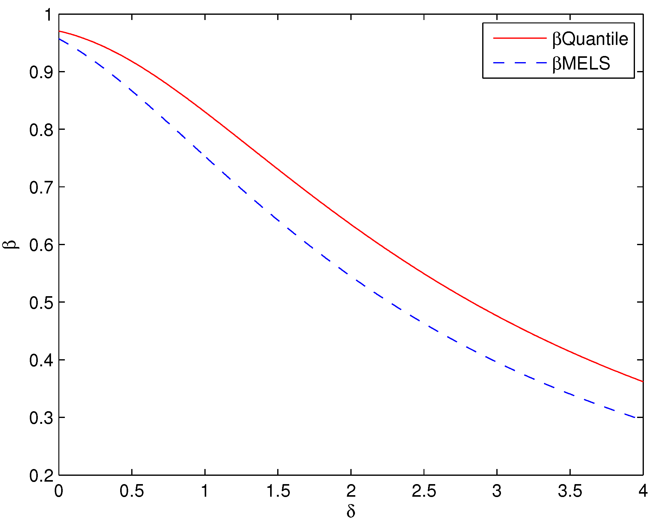
Based on the ME distribution approximation to the distribution of the monitored quantity, with , the control limits and the acceptance regions (UCL–LCL) of the three charts are shown in Table 5. Furthermore, it is obvious that the volume of acceptance region in the simplified MELS chart appears much smaller than the Quantile chart. Although the conventional Shewhart chart has the smallest volume of acceptance region with , it is very unreasonable to use the Shewhart chart in this case. First, with its acceptance region, the actual is much smaller than 0.05 for this asymmetric distribution here. Furthermore, the value of LCL for the Shewhart chart is which contradicts the non-negative quantity X (see Equation (18)). Hence, the comparison of Type II error rates is just presented between the simplified MElS chart and the Quantile chart. Suppose the distribution of out-of-control X is the same as Equation (19), and the Type II error rates of the two control charts are plotted for each in Figure 4. From Figure 4, it is clear that the Type II error rates for the simplified MELS chart are much lower than the Quantile chart. This helps to improve the capacity of detecting the shifts for the monitored quantity better than the Quantile chart. Thus, comparing to the conventional charts, the simplified MELS control chart performs more effectively for monitoring the quantity with unimodal distribution.
5. Discussion
Theoretically, the acceptance regions are supposed to be totally equivalent in the situation of symmetric distribution. The divergences among the three acceptance regions are mainly attributed to the incomplete ME density approximation of the true density (see Table 1). With the improvement of optimization techniques, the ME distribution and the true distribution tend to overlap (see Figure 1). Hence, for most symmetric distribution situations, once the sample size for conventional control charts design is required (see [25]).
For the asymmetric unimodal distribution, given a specified Type I error rate , the acceptance regions obtained by the simplified MELS chart have lower Type II error rates (see Figure 3 and Figure 4) whatever the unknown distribution of monitored quantity is approximated by the true distribution or ME distribution. The lower Type II error rate can improve the higher detection capability for the control chart, thus the simplified MELS chart performs much better than the Shewhart chart and the Quantile chart when the monitored quantity is the asymmetric unimodal distribution.
The advantages of application of the simplified MELS chart are found as follows: (i) For the monitored quantity with unknown distribution in SPC, it can be used to establish the control chart without making an assumption of the distribution of the monitored quantity. (ii) For the monitored quantity with unimodal distribution, it is easier and more convenient for the users to decide the optimal in-control region compared to the existing MELS chart. (iii) It has a higher detection capability than the conventional control charts for the monitored quantity with asymmetric unimodal distribution. (iv) It can be widely used for the nonparametric control chart design in manufacturing, such as the products’ processing control quality attributes such as the length, weight, purity, time, output, etc., even the service quality attributes such as the responsiveness, assurance and reliability.
The effectiveness of the simplified MELS method depends a lot on the approximation degree between the ME density and the true density. Thus, the big challenge for the proposed method is the optimization of the Lagrange multipliers in ME distribution estimation. We can see that the differences between the true density and the ME density in Figure 2 are larger than that in Figure 1, because the optimization for is much more difficult in asymmetric unimodal distribution than in the case of symmetric distribution. In ME density estimation, the higher order moment constraints can help to mine much more information about the monitored quantity, but they also cause a more complicated optimization problem. Thus, in future work, the number of order moments in ME density estimation is a difficult problem that still needs further research. Besides, improving the optimization algorithm in ME density estimation is another way to increase the effectiveness of the MELS/simplified MELS method, and we can try to utilize intelligence algorithms such as the genetic algorithm to improve the optimization results.
6. Conclusions
A novel attempt has been made to propose a simplified MELS chart for the unimodal distribution of the monitored quantity in this article. First, the distribution of the monitored quantity is approximated by the ME density. Then, instead of in the MELS chart, X is taken directly as the monitoring statistic in the proposed method. Finally, under the Type I error rate , the ME density level set with the minimum volume of X is considered as the optimal in-control region. Thus, compared to the MELS chart, the acceptance region for monitored quantity in the simplified MELS chart is more convenient to establish and it is easier for the users to implement. The results from the case study have validated that the simplified MELS chart performs better than the Shewhart chart and the Quantile chart for the monitored quantity with asymmetric unimodal distribution.
Acknowledgments
The authors would like thank the financial supports by the National Natural Science Foundation of China (Grant No. 71471107) and Zhejiang Provinvcial Natural Science Foundation of China (Grant No. LY17G030028). The authors also thank the Cllaborative Innovation Center of Standardization and Intellectual Property Management of Zhejiang (Grant No. SIPM3207).
Author Contributions
Xinghua Fang proposed the method and wrote the main manuscript text. Mingshun Song conceived and designed the expriments. Yizeng Chen contributed to the formula deduction and adjustment of the article structure.
Conflicts of Interest
The authors declare no conflict of interest.
References
- Saniga, E.; Davis, D.; Lucas, J. Using Shewhart and CUSUM charts for diagnosis with count data in a ventor certification study. J. Qual. Technol. 2009, 41, 217–227. [Google Scholar]
- Runger, G.C.; Testik, M.C. Multivariate extensions to cumulative sum control charts. Qual. Reliab. Eng. Int. 2004, 20, 587–606. [Google Scholar] [CrossRef]
- Tan Matthias, H.; Shi, J. A bayesian approach for interpreting mean shifts in multivariate quality control. Technometrics 2014, 54, 294–307. [Google Scholar]
- Calabrese, J. Bayesian process control for attributes. Manag. Sci. 1995, 41, 637–645. [Google Scholar] [CrossRef]
- Apley, D.W. Posterior distribution charts: A bayesian approach for graphically exploring a process mean. Technometrics 2012, 54, 279–293. [Google Scholar] [CrossRef]
- Das, D.; Zhou, S. Statistical process monitoring based on maximum entropy density approximation and level set principle. IIE Trans. 2015, 47, 215–229. [Google Scholar] [CrossRef]
- Apley, D.W.; Tsung, F. The autoregressive T2 chart for monitoring univariate autocorrelated process. J. Qual. Technol. 2002, 34, 80–96. [Google Scholar]
- Bersimis, S.; Psarakis, S.; Panaretos, J. Multivariate statistical process control charts: An overview. Qual. Reliab. Eng. Int. 2007, 23, 517–543. [Google Scholar] [CrossRef] [Green Version]
- Zhou, M.; Zhou, Z.; Geng, W. A new nonparametric control chart for monitoring variability. Qual. Reliab. Eng. Int. 2016, 32, 2471–2479. [Google Scholar] [CrossRef]
- Acharya, U.; Fujita, H.; Sudarshan, V.; Bhat, S.; Koh, J. Apllication of entropies for automated diagnosis of epilepsy using EEG signals: A review. Knowl.-Based Syst. 2015, 88, 85–96. [Google Scholar] [CrossRef]
- Acharya, U.; Molinari, F.; Sree, S.; Chattopadhyay, S.; Ng, K.; Suri, J. Automated diagnosis of epilepsy EEG using Entropies. Biomed. Signal Process. Control 2012, 7, 401–408. [Google Scholar] [CrossRef]
- Alwan, L.C.; Ebrahimi, N; Soofi, E.S. Information theoretic framework for process control. Eur. J. Oper. Res. 1998, 111, 336–347. [Google Scholar] [CrossRef]
- Jaynes, E. Information theory and statistical mechanics. Phys. Rev. 1957, 106, 19–31. [Google Scholar] [CrossRef]
- Shannon, C. A mathmatical theory of communication. Bell. Syst. Tech. J. 1948, 27, 379–423, 623–656. [Google Scholar] [CrossRef]
- Nieves, V.; Wang, J.; Bras, B.; Wood, E. Maximum entropy distribution of scale-invariant processes. Phys. Rev. Lett. 2010, 105, 118701. [Google Scholar] [CrossRef] [PubMed]
- Alves, A.; Dias, A.; da Silva, R. Maximum entropy principle and the Higgs boson mass. Physica A 2015, 420, 1–7. [Google Scholar] [CrossRef]
- Neri, C.; Schneider, L. Maximum entropy distributions inferred from option profolios on an asset. Financ. Stoch. 2012, 16, 293–318. [Google Scholar] [CrossRef]
- Tanaka, K.; Toda, A. Discrete approximations of continous distributions by maximum entropy. Econ. Lett. 2013, 118, 445–450. [Google Scholar] [CrossRef]
- Barzdajn, B. Maximum entropy distribution under moments and quantiles constraits. Measurement 2014, 52, 102–107. [Google Scholar] [CrossRef]
- Batou, A.; Soize, C. Generation of accelerograms compatible with design specifications using information theory. Bull. Earthq. Eng. 2014, 12, 769–794. [Google Scholar] [CrossRef]
- Zhu, H.; Zuo, Y.; Li, X.; Deng, J.; Zhuang, X. Estimation of the fracture diameter diatribution using the maximum entropy principle. Int. J. Rock Mech. Min. Sci. 2014, 72, 127–137. [Google Scholar]
- Abramov, R. An imroved algrotithm for the multidimensional moment-constrained maximum entropy problem. J. Comput. Phys. 2007, 226, 621–644. [Google Scholar] [CrossRef]
- Park, C.; Huang, J.; Ding, Y. A computable plug-in estimator of minimum volume sets for novelty detection. Oper. Res. 2010, 58, 1469–1480. [Google Scholar] [CrossRef]
- Garcia, J.; Kutalik, Z.; Cho, K.; Wolkenhauer, O. Level sets and minimum volume sets of probability density functions. Int. J. Approx. Reason. 2003, 34, 25–47. [Google Scholar] [CrossRef]
- Besterfield, D. Quality Control, 8th ed.; Pearson: Upper Saddle River, NJ, USA, 2009; pp. 187–207. [Google Scholar]
Figure 1.
Density functions of the symmetric unimodal distribution.
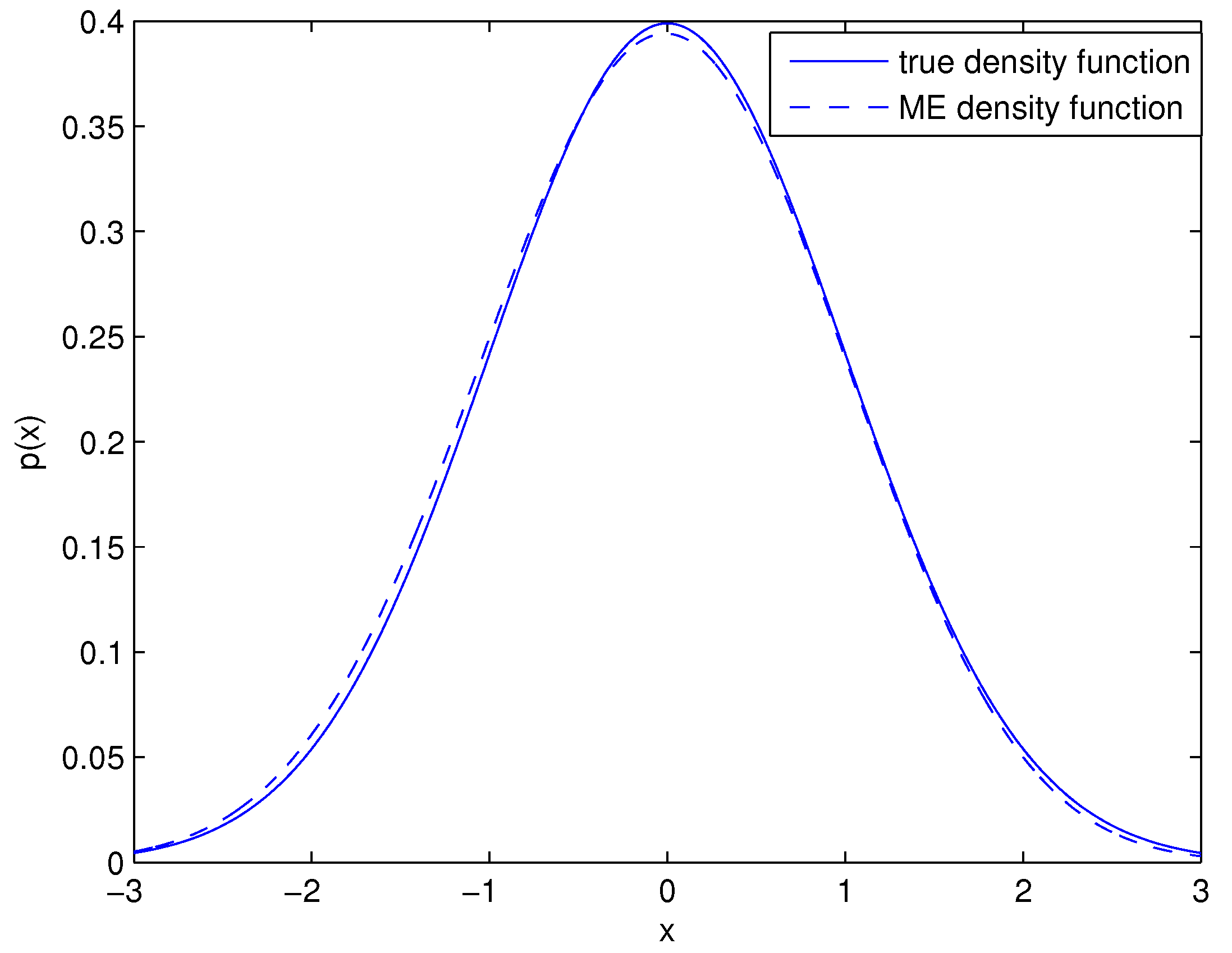
Figure 2.
Density functions for the asymmetric unimodal distribution.
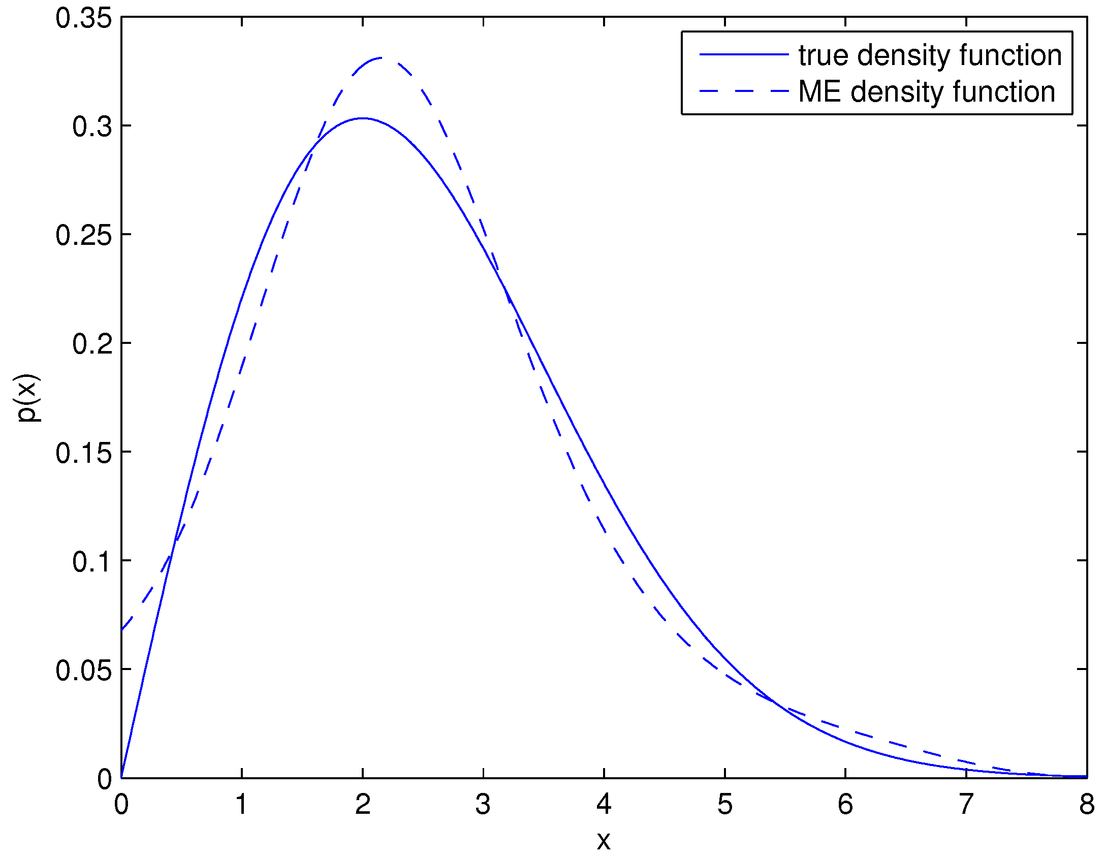
Figure 3.
Type II error for the asymmetric unimodal distribution based on true distribution.
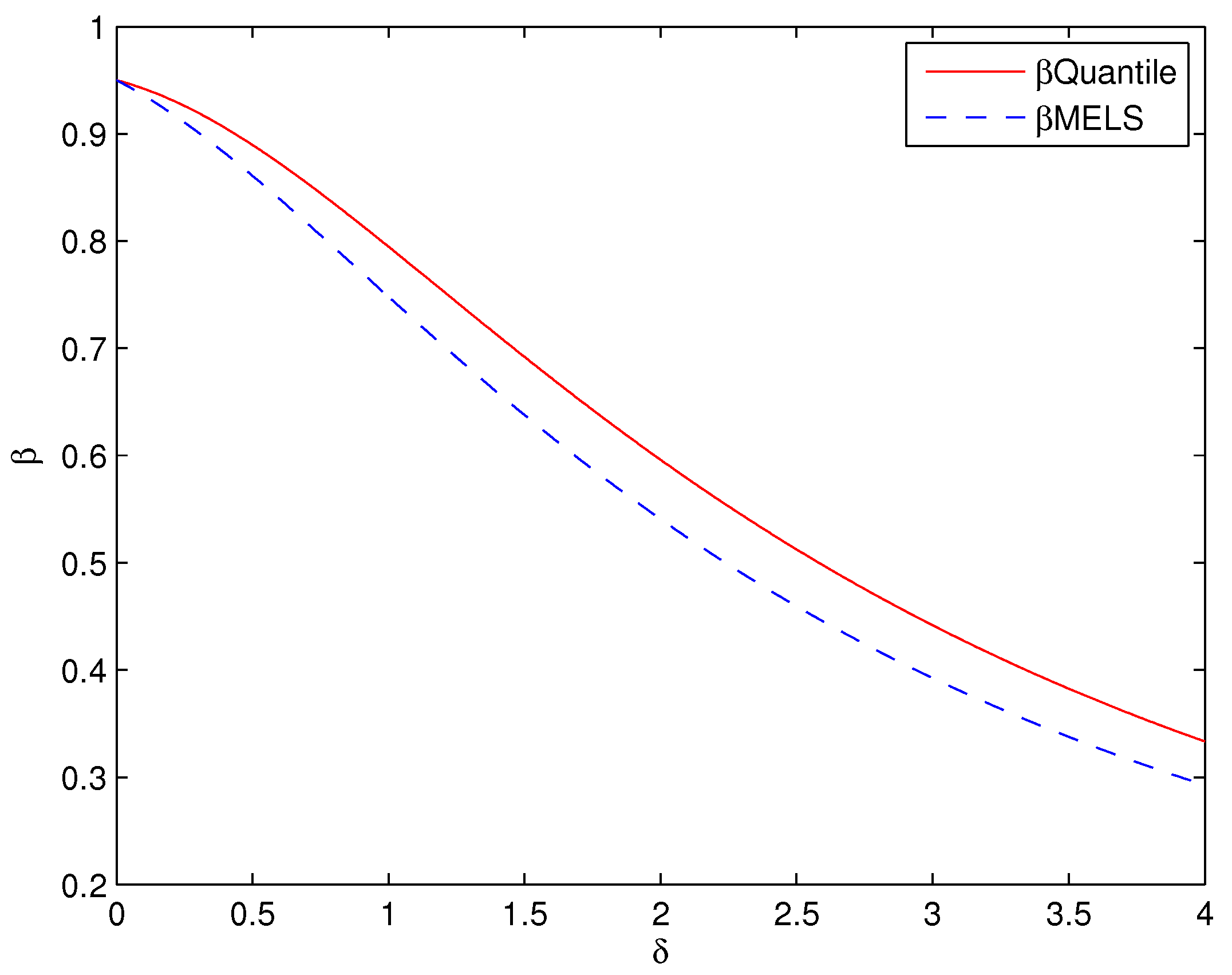
Figure 4.
Type II error for the asymmetric unimodal distribution based on ME distribution.


Table 1.
Parameters of Maximum Entropy (ME) density for symmetric unimodal distribution.
| i | 0 | l | 2 | 3 | 4 | 5 |
|---|---|---|---|---|---|---|
| 1 | ||||||
Table 2.
Control limits of the three control charts for symmetric unimodal distribution.
| LCL | UCL | UCL–LCL | |
|---|---|---|---|
| Shewhart | −1.9600 | 1.9600 | 3.9200 |
| MELS | −1.9300 | 1.9500 | 3.8800 |
| Quantile | −1.9621 | 1.9570 | 3.9191 |
Table 3.
Control limits of the two control charts for asymmetric unimodal distribution.
| LCL | UCL | UCL–LCL | |
|---|---|---|---|
| MELS | 0.2212 | 5.0007 | 4.7795 |
| Quantile | 0.4500 | 5.4324 | 4.9824 |
Table 4.
Parameters of ME density for the asymmetric unimodal distribution.
| i | 0 | l | 2 | 3 | 4 | 5 |
|---|---|---|---|---|---|---|
| 1 | 2.5083 | 7.9761 | 30.8721 | 128.1232 | 591.5907 | |
| −2.6913 | 0.9143 | 0.3876 | −0.3339 | 0.0614 | −0.0036 |
Table 5.
Control limits of the three control charts for the asymmetric unimodal distribution.
| LCL | UCL | UCL–LCL | |
|---|---|---|---|
| Shewhart | 5.0735 | 4.5213 | |
| MELS | 0.0000 | 5.0180 | 5.0180 |
| Quantile | 0.3150 | 5.7012 | 5.3862 |
© 2017 by the authors. Licensee MDPI, Basel, Switzerland. This article is an open access article distributed under the terms and conditions of the Creative Commons Attribution (CC BY) license (http://creativecommons.org/licenses/by/4.0/).
Share and Cite
MDPI and ACS Style
Fang, X.; Song, M.; Chen, Y. Statistical Process Control for Unimodal Distribution Based on Maximum Entropy Distribution Approximation. Entropy 2017, 19, 406. https://doi.org/10.3390/e19080406
AMA Style
Fang X, Song M, Chen Y. Statistical Process Control for Unimodal Distribution Based on Maximum Entropy Distribution Approximation. Entropy. 2017; 19(8):406. https://doi.org/10.3390/e19080406
Chicago/Turabian StyleFang, Xinghua, Mingshun Song, and Yizeng Chen. 2017. "Statistical Process Control for Unimodal Distribution Based on Maximum Entropy Distribution Approximation" Entropy 19, no. 8: 406. https://doi.org/10.3390/e19080406
Note that from the first issue of 2016, this journal uses article numbers instead of page numbers. See further details here.