A View of Information-Estimation Relations in Gaussian Networks


1
Department of Electrical Engineering, Princeton University, Princeton, NJ 08544, USA
2
Department of Electrical Engineering, Technion-Israel Institute of Technology, Haifa 32000, Israel
*
Authors to whom correspondence should be addressed.
Entropy 2017, 19(8), 409; https://doi.org/10.3390/e19080409
Submission received: 31 May 2017
/
Revised: 31 July 2017
/
Accepted: 1 August 2017
/
Published: 9 August 2017
(This article belongs to the Special Issue Network Information Theory)
Abstract
:Relations between estimation and information measures have received considerable attention from the information theory community. One of the most notable such relationships is the I-MMSE identity of Guo, Shamai and Verdú that connects the mutual information and the minimum mean square error (MMSE). This paper reviews several applications of the I-MMSE relationship to information theoretic problems arising in connection with multi-user channel coding. The goal of this paper is to review the different techniques used on such problems, as well as to emphasize the added-value obtained from the information-estimation point of view.
1. Introduction
The connections between information theory and estimation theory go back to the late 1950s in the work of Stam in which he uses the de Bruijn identity [1], attributed to his PhD advisor, which connects the differential entropy and the Fisher information of a random variable contaminated by additive white Gaussian noise. In 1968 Esposito [2] and then in 1971 Hatsell and Nolte [3] identified connections between the Laplacian and the gradient of the log-likelihood ratio and the conditional mean estimate. Information theoretic measure can indeed be put in terms of log-likelihood ratios, however, these works did not make this additional connecting step. In the early 1970s continuous-time signals observed in white Gaussian noise received specific attention in the work of Duncan [4] and Kadota et al. [5] who investigated connections between the mutual information and causal filtering. In particular, Duncan and Zakai (Duncan’s theorem was independently obtained by Zakai in the general setting of inputs that may depend causally on the noisy output in a 1969 unpublished Bell Labs Memorandum (see [6])) [4,7] showed that the input-output mutual information can be expressed as a time integral of the causal minimum mean square error (MMSE). It was only in 2005 that Guo, Shamai and Verdú revealed the I-MMSE relationship [8], which similarly to the de Bruijn identity, relates information theoretic quantities to estimation theoretic quantities over the additive white Gaussian noise channel. Moreover, the fact that the I-MMSE relationship connects the mutual information with the MMSE has made it considerably more applicable, specifically to information theoretic problems.
The I-MMSE type relationships have received considerable attention from the information theory community and a number of extensions have been found. In [9], in the context of multiple-input multiple-output (MIMO) Gaussian channels, it was shown that the gradient of the mutual information with respect to the channel matrix is equal to the channel matrix times the MMSE matrix. In [10] a version of the I-MMSE identity has been shown for Gaussian channels with feedback. An I-MMSE type relationship has been found for additive non-Gaussian channels in [11] and non-additive channels with a well-defined notion of the signal-to noise ratio (SNR) in [12,13,14,15]. A relationship between the MMSE and the relative entropy has been established in [16], and between the score function and Rényi divergence and f-divergence in [17]. The I-MMSE relationship has been extended to continuous time channels in [8] and generalized in [18] by using Malliavin calculus. For other continuous time generalizations the reader is referred to [19,20,21]. Finally, Venkat and Weissman [22] dispensed with the expectation and provided a point-wise identity that has given additional insight into this relationship. For a comprehensive summary of results on the interplay between estimation and information measures the interested reader is referred to [23].
In this survey we provide an overview of several applications of the I-MMSE relationship to multi-user information theoretic problems. We consider three types of applications:
- Capacity questions, including both converse proofs and bounds given additional constraints such as discrete inputs;
- The MMSE SNR-evolution, meaning the behavior of the MMSE as a function of SNR for asymptotically optimal code sequences (code sequences that approach capacity as ); and
- Finite blocklength effects on the SNR-evolution of the MMSE and hence effects on the rate as well.
Our goal in this survey is both to show the strength of the I-MMSE relationship as a tool to tackle network information theory problems, and to overview the set of tools used in conjunction with the I-MMSE relationship such as the “single crossing point” property. As will be seen such tools lead to alternative and, in many cases, simpler proofs of information theoretic converses.
We are also interested in using estimation measures in order to upper or lower bound information measures. Such bounds lead to simple yet powerful techniques that are used to find “good” capacity approximations. At the heart of this technique is a generalization of the Ozarow-Wyner bound [24] based on minimum mean p-th error (MMPE). We hope that this overview will enable future application of these properties in additional multi-user information theoretic problems.
The outline of the paper is as follows:
- In Section 2 we review information and estimation theoretic tools that are necessary for the presentation of the main results.
- In Section 3 we go over point-to-point information theory and give the following results:
- In Section 3.1, using the I-MMSE and a basic MMSE bound, a simple converse is shown for the Gaussian point-to-point channel;
- In Section 3.2, a lower bound, termed the Ozarow-Wyner bound, on the mutual information achieved by a discrete input on an AWGN channel, is presented. The bound holds for vector discrete inputs and yields the sharpest known version of this bound; and
- In Section 3.3, it is shown that the MMSE can be used to identify optimal point-to-point codes. In particular, it is shown that an optimal point-to-point code has a unique SNR-evolution of the MMSE.
- In Section 4 we focus on the wiretap channel and give the following results:
- In Section 4.1, using estimation theoretic properties a simple converse is shown for the Gaussian wiretap channel that avoids the use of the entropy power inequality (EPI); and
- In Section 4.2, some results on the SNR-evolution of the code sequences for the Gaussian wiretap channel are provided, showing that for the secrecy capacity achieving sequences of codes the SNR-evolution is unique.
- In Section 5 we study a communication problem in which the transmitter wishes to maximize its communication rate, while subjected to a constraint on the disturbance it inflicts on the secondary receiver. We refer to such scenarios as communication with a disturbance constraint and give the following results:
- In Section 5.1 it is argued that an instance of a disturbance constraint problem, when the disturbance is measured by the MMSE, has an important connection to the capacity of a two-user Gaussian interference channel;
- In Section 5.2 the capacity is characterized for the disturbance problem when the disturbance is measured by the MMSE;
- In Section 5.3 the capacity is characterized for the disturbance problem when the disturbance is measured by the mutual information. The MMSE and the mutual information disturbance results are compared. It is argued that the MMSE disturbance constraint is a more natural measure in the case when the disturbance measure is chosen to model the unintended interference;
- In Section 5.4 new bounds on the MMSE are derived and are used to show upper bounds on the disturbance constraint problem with the MMSE constraint when the block length is finite; and
- In Section 5.5 a notion of mixed inputs is defined and is used to show lower bounds on the rates of the disturbance constraint problem when the block length is finite.
- In Section 6 we focus on the broadcast channel and give the following results:
- In Section 6.1, the converse for a scalar Gaussian broadcast channel, which is based only on the estimation theoretic bounds and avoids the use of the EPI, is derived; and
- In Section 6.2, similarly to the Gaussian wiretap channel, we examine the SNR-evolution of asymptotically optimal code sequences for the Gaussian broadcast channel, and show that any such sequence has a unique SNR-evolution of the MMSE.
- In Section 7 the SNR-evolution of the MMSE is derived for the K-user broadcast channel.
- In Section 8, building on the MMSE disturbance problem in Section 5.1, it is shown that for the two-user Gaussian interference channel a simple transmission strategy of treating interference as noise is approximately optimal.
Section 9 concludes the survey by pointing out interesting future directions.
1.1. Notation
Throughout the paper we adopt the following notational conventions:
- Random variables and vectors are denoted by upper case and bold upper case letters, respectively, where r.v. is short for either random variable or random vector, which should be clear from the context. The dimension of these random vectors is n throughout the survey. Matrices are denoted by bold upper case letters;
- If A is an r.v. we denote the support of its distribution by ;
- The symbol may denote different things: is the determinant of the matrix , is the cardinality of the set , is the cardinality of , or is the absolute value of the real-valued x;
- The symbol denotes the Euclidian norm;
- denotes the expectation;
- denotes the density of a real-valued Gaussian r.v. with mean vector and covariance matrix ;
- denotes the uniform probability mass function over a zero-mean pulse amplitude modulation (PAM) constellation with points, minimum distance , and therefore average energy ;
- The identity matrix is denoted by ;
- The reflection of the matrix along its main diagonal, or the transpose operation, is denoted by ;
- The trace operation on the matrix is denoted by ;
- The order notation implies that is a positive semidefinite matrix;
- denotes the logarithm to the base ;
- is the set of integers from to ;
- For we let denote the largest integer not greater than x;
- For we let and ;
- Let be two real-valued functions. We use the Landau notation to mean that for some there exists an such that for all , and to mean that for every there exists an such that for all ; and
- We denote the upper incomplete gamma function and the gamma function by
2. Estimation and Information Theoretic Tools
In this section, we overview relevant information and estimation theoretic tools. The specific focus is to show how estimation theoretic measures can be used to represent or bound information theoretic measures such as entropy and mutual information.
2.1. Estimation Theoretic Measures
Of central interest to us is the following estimation measure constructed from the norm.
Definition 1.
For the random vector and let
We define the minimum mean p-th error (MMPE) of estimating from as
where the minimization is over all possible Borel measurable functions . Whenever the optimal MMPE estimator exists, we shall denote it by .
In particular, for the norm in (2a) is given by
and for uniform over the n dimensional ball of radius r the norm in (2a) is given by
We shall denote
if and are related as
where , is independent of , and is the SNR. When it will be necessary to emphasize the SNR at the output , we will denote it by . Since the distribution of the noise is fixed is completely determined by the distribution of and and there is no ambiguity in using the notation . Applications to the Gaussian noise channel will be the main focus of this paper.
In the special, case when , we refer to the MMPE as the minimum mean square error (MMSE) and use the notation
in which case we also have that .
Remark 1.
The notation , for the optimal estimator in (2) is inspired by the conditional expectation , and should be thought of as an operator on and a function of . Indeed, for , the MMPE reduces to the MMSE; that is, and .
Finally, similarly to the conditional expectation, the notation should be understood as an evaluation for a realization of a random variable , while should be understood as a function of a random variable which itself is a random variable.
Lemma 1.
In certain cases the optimal estimator might not be unique and the interested reader is referred to [25] for such examples. In general we do not have a closed form solution for the MMPE optimal estimator in (2). Interestingly, the optimal estimator for Gaussian inputs can be found and is linear for all
Note that unlike the Gaussian case in general the estimator will be a function of the order p. For equally likely (i.e., binary phase shift keying—BPSK) the optimal estimator is given by
Often the MMPE is difficult to compute, even for (MMSE), and one instead is interested in deriving upper bounds on the MMPE. One of the most useful upper bounds on the MMPE can be obtained by restricting the optimization in (2) to linear functions.
Proposition 2.
(Asymptotically Gaussian is the “hardest” to estimate [25]) For , , and a random variable such that , we have
where
Moreover, a Gaussian with per-dimension variance (i.e., ) asymptotically achieves the bound in (10a), since .
For the case of , the bound in (10a) is achieved with a Gaussian input for all SNR’s. Moreover, this special case of the bound in (10a), namely
for all , is referred to as the linear minimum mean square error (LMMSE) upper bound.
2.2. Mutual Information and the I-MMSE
For two random variables distributed according to the mutual information is defined as
where is the Radon-Nikodym derivative. For the channel in (6) the mutual information between and takes the following form:
and it will be convenient to use the normalized mutual information
The basis for much of our analysis is the fundamental relationship between information theory and estimation theory, also known as the Guo, Shamai and Verdú I-MMSE relationship [8].
Theorem 1.
In [28] the I-MMSE relationship has been partially extended to the limit as . This result was then extended in [29] under the assumption that the mutual information sequence converges.
Proposition 3.
(I-MMSE limiting expression [29]) Suppose that and
exists. (The limit here is taken with respect to a sequence of input distributions over which induces a sequence of input-output joint distributions. The second moment constraint should be understood in a similar manner, as a constraint for every n in the sequence.) Then,
and the I-MMSE relationship holds for the following limiting expression:
Proof.
The proof is given in Appendix A. ☐
Properties of the MMSE, with the specific focus on the I-MMSE identity, as a function of the input distribution and the noise distribution have been thoroughly studied and the interested reader is referred to [17,30,31,32]. For the derivation of the I-MMSE and a comprehensive summary of various extension we refer the reader to [23].
For a continuous random vector with the density the differential entropy is defined as
Moreover, for a discrete random vector the discrete entropy is defined as
2.3. Single Crossing Point Property
Upper bounds on the MMSE are useful, thanks to the I-MMSE relationship, as tools to derive information theoretic converse results, and have been used in [23,30,33,34] to name a few. The key MMSE upper bound that will be used in conjunction with the I-MMSE to derive information theoretic converses is the single crossing point property (SCPP).
Proposition 4.
Even though the statement of Proposition 4 seems quite simple it turns out that it is sufficient to show a special case of the EPI [33]:
where . Interestingly, the I-MMSE appears to be a very powerful tool in deriving EPI type inequalities; the interested reader is referred to [35,36,37,38].
In [25] it has been pointed out that the SCPP upper bound can also be shown for the MMPE as follows.
Proposition 5.
Proof.
The proof of Propositions 4 and 5 uses a clever choice of a sub-optimal estimator. The interested reader is referred to Appendix B for the proof. ☐
2.4. Complementary SCPP Bounds
Note that the SCPP allows us to upper bound the MMSE for all values of , and as will be shown later this is a very powerful tool in showing information theoretic converses. Another interesting question is whether we can produce a complementary upper bound to that of the SCPP. That is, can we show an upper bounds on the MMSE for ? As will be demonstrated in Section 5, such complementary SCPP bounds are useful in deriving information theoretic converses for problems of communication with a disturbance constraint.
The next result shows that this is indeed possible.
Proposition 6.
(Complementary SCPP bound [25]) For , and , we have
An interesting property of the bound in Proposition 6 is that the right hand side of the inequality keeps the channel SNR fixed and only varies the order of the MMPE while the left hand side of the inequality keeps the order fixed and changes the SNR value.
2.5. Bounds on Differential Entropy
Another common application of estimation theoretic measures is to bound information measures. Next, we presented one such bound.
For any random vector such that and any random vector , the following inequality is considered to be a continuous analog of Fano’s inequality [39]:
where the inequality in (25) is a consequence of the arithmetic-mean geometric-mean inequality, that is, for any we have used where ’s are the eigenvalues of .
The inequality in (25) can be generalized in the following way.
Theorem 2.
While the MMPE is still a relatively new tool it has already found several applications:
- The MMPE can be used to bound the conditional entropy (see Theorem 2 in Section 2.5). These bounds are generally tighter than the MMSE based bound especially for highly non-Gaussian statistics;
- The MMPE can be used to develop bounds on the mutual information of discrete inputs via the generalized Ozarow-Wyner bound (see Theorem 4 in Section 3.2); The MMPE and the Ozarow-Wyner bound can be used to give tighter bounds on the gap to capacity achieved by PAM input constellations (see Figure 2);
- The MMPE can be used as a key tool in finding complementary bounds on the SCPP (see Theorem 10 in Section 5.4). Note that using the MMPE as a tool produces the correct phase transition behavior; and
- While not mentioned, another application is to use the MMPE to bound the derivatives of the MMSE; see [25] for further details.
3. Point-to-Point Channels
In this section, we review Shannon’s basic theorem for point-to-point communication and introduce relevant definitions used throughout the paper. The point-to-point channel is also a good starting point for introducing many of the techniques that will be used in this survey.
A classical point-to-point channel is shown in Figure 1. The transmitter wishes to reliably communicate a message W at a rate R bits per transmission to a receiver over a noisy channel. To that end, the transmitter encodes the message W into a signal and transmits it over a channel in n time instances. Upon receiving a sequence , a corrupted version of , the receiver decodes it to obtain the estimate .
Definition 2.
A memoryless channel (MC), assuming no feedback, (in short ) consists of an input set , an output set , and a collection of transition probabilities on for every . The transition of a length-n vector through such a channel then has the following conditional distribution:
Definition 3.
A code of length n and rate R, denoted by , of the channel consist of the following:
- A message set. We assume that the message W is chosen uniformly over the message set.
- An encoding function that maps messages W to codewords . The set of all codewords is called the codebook and is denoted by ; and
- A decoding function that assigns an estimate to each received sequence.
The average probability of error for a code is defined as
Definition 4.
A rate R is said to be achievable over a point-to-point channel if there exists a sequence of codes, , such that
The capacity C of a point-to-point channel is the supremum over all achievable rates.
A crowning achievement of Shannon’s 1948 paper [40] is a simple characterization of the capacity of a point-to-point channel.
Theorem 3.
(Channel Coding Theorem [40]) The capacity of the channel is given by
For a formal derivation of the capacity expression in (29) the reader is referred to classical texts such as [39,41,42].
3.1. A Gaussian Point-to-Point Channel
In this section we consider the practically relevant Gaussian point-to-point channel shown in Figure 1b and given by
where Z is standard Gaussian noise and there is an additional input power constraint . The capacity in this setting was solved in the original paper by Shannon and is given by
To show the converse proof of the capacity (the upper bound on the capacity) in (31), Shannon used the maximum entropy principle. In contrast to Shannon’s proof, we show the converse can be derived by using the I-MMSE and the LMMSE upper bound in (11)
It is well know that the upper bound in (32) is achievable if and only if the input is .
The main idea behind the upper bounding technique in (32) is to find an upper bound on the MMSE that holds for all SNR’s and integrate it to get an upper bound on the mutual information. This simple, yet powerful, idea will be used many times throughout this paper to show information theoretic converses for multi-user channels.
3.2. Generalized Ozarow-Wyner Bound
In practice, Gaussian inputs are seldom used and it is important to assess the performance of more practical discrete constellations (or inputs). Another reason is that discrete inputs often outperform Gaussian inputs in competitive multi-user scenarios, such as the interference channel, as will be demonstrated in Section 7. For other examples of discrete inputs being useful in multi-user settings, the interested readers is referred to [43,44,45,46].
However, computing an exact expression for the mutual information between the channel input and output when the inputs are discrete is often impractical or impossible. Therefore, the goal is to derive a good computable lower bound on the mutual information that is not too far away from the true value of the mutual information. As we will see shortly, estimation measures such as the MMSE and the MMPE will play an important role in establishing good lower bounds on the mutual information.
The idea of finding good capacity approximations can be traced back to Shannon. Shannon showed, in his unpublished work in 1948 [47], the asymptotic optimality of a PAM input for the point-to-point power-constrained Gaussian noise channel. Another such observation about approximate optimality of a PAM input was made by Ungerboeck in [48] who, through numerical methods, observed that the rate of a properly chosen PAM input is always a constant away from the AWGN capacity.
Shannon’s and Ungerboeck’s arguments were solidified by Ozarow and Wyner in [24] where firm lower bounds on the achievable rate with a PAM input were derived and used to show optimality of PAM to within 0.41 bits [24].
In [24] the following “Ozarow-Wyner lower bound” on the mutual information achieved by a discrete input transmitted over an AWGN channel was shown:
where is the LMMSE. The advantage of the bound in (33) compared to the existing bounds is its computational simplicity. The bound depends only on the entropy, the LMMSE, and the minimum distance, which are usually easy to compute.
The bound in (33) has also been proven to be useful for other problems such as two-user Gaussian interference channels [45,49], communication with a disturbance constraint [50], energy harvesting problems [51,52], and information-theoretic security [53].
The bound on the in (33) has been sharpened in [45] to
since .
Finally, the following generalization of the bound in (34) to discrete vector input, which is the sharpest known bound on the term, was derived in [25].
Theorem 4.
(Generalized Ozarow-Wyner Bound [25]) Let be a discrete random vector with finite entropy, and let be a set of continuous random vectors, independent of , such that for every , , and
Then for any
where
Remark 2.
The condition in (35a) can be enforced by, for example, selecting the support of to satisfy a non-overlap condition given by
as was done in [54].
It is interesting to note that the lower bound in (35b) resembles the bound for lattice codes in [55], where can be thought of as a dither, corresponds to the log of the normalized p-moment of a compact region in , corresponds to the log of the normalized MMSE term, and corresponds to the capacity C.
In order to show the advantage of Theorem 4 over the original Ozarow-Wyner bound (case of and with LMMSE instead of MMPE), we consider uniformly distributed with the number of points equal to , that is, we choose the number of points such that . Figure 2 shows:
- The solid cyan line is the “shaping loss” for a one-dimensional infinite lattice and is the limiting gap if the number of points N grows faster than ;
- The solid magenta line is the gap in the original Ozarow-Wyner bound in (33); and
- The dashed purple, dashed-dotted blue and dotted green lines are the new gap given by Theorem 4 for values of , respectively, and where we choose .
We note that the version of the Ozarow-Wyner bound in Theorem 4 provides the sharpest bound for the gap term. An open question, for , is what value of p provide the smallest gap and whether it coincides with the ultimate “shaping loss”.
For the AWGN channel there exist a number of other bounds that use discrete inputs as well (see [46,56,57,58] and references therein). The advantage of using Ozarow-Wyner type bounds, however, lies in their simplicity as they only depend on the number of signal constellation points and the minimum distance of the constellation.
3.3. SNR Evolution of Optimal Codes
The I-MMSE can also be used in the analysis of the MMSE SNR-evolution of asymptotically optimal code sequences (code sequences that approach capacity in the limit of blocklength). In particular, using the I-MMSE relationship one can exactly identify the MMSE SNR-evolution of asymptotically optimal code sequences for the Gaussian point-to-point channel.
Theorem 5.
Figure 3 depicts the SNR evolution of the MMSE as described in Theorem 5. The discontinuity of the MMSE at is ofter referred to as the phase transition. From Theorem 5 it is clear that the optimal point-to-point code must have the same MMSE profile as the Gaussian distribution for all SNR’s before and experience a phase transition at . Intuitively, the phase transition happens because an optimal point-to-point code designed to operate at can be reliably decoded at and SNR’s larger than , and both the decoding and estimation errors can be driven to zero. It is also important to point out that the area under (37) is twice the capacity.
4. Applications to the Wiretap Channel
In this section, by focusing on the wiretap channel, it is shown how estimation theoretic techniques can be applied to multi-user information theory. The wiretap channel, introduced by Wyner in [64], is a point-to-point channel with an additional eavesdropper (see Figure 4a). The input is denoted by , the output of the legitimate user is denoted by , and the output of an eavesdropper is denoted by . The transmitter of , commonly referred to as Alice, wants to reliably communicate a message W to the legitimate receiver , commonly referred to as Bob, while keeping the message W secure to some extent from the eavesdropper , commonly referred to as Eve.
Definition 5.
A rate-equivocation pair is said to be achievable over a wiretap channel if there exists a sequence of codes such that
The rate-equivocation region is defined as the closure of all achievable rate-equivocation pairs, and the secrecy capacity is defined as
The secrecy capacity of a general wiretap channel was shown by Csiszár and Körner [65] and is given by
where U is an auxiliary random variable that satisfies the Markov relationship .
In the case of a degraded wiretap channel (i.e., a wiretap channel obeying the Markov relationship ) the expression in (40) reduces to
In fact, the expression in (41) for the degraded channel predates the expression in (40) and was shown in the original work of Wyner [64].
4.1. Converse of the Gaussian Wiretap Channel
In this section, we consider the practically relevant scalar Gaussian wiretap channel given by
where , with an additional input power constraint . This setting was considered in [66], and the secrecy capacity was shown to be
In contrast to the proof in [66], where the key technical tool used to maximize the expression in (41) was the EPI, by using the I-MMSE relationship the capacity in (43) can be shown via the following simple three line argument [30]:
where the inequality follows by using the LMMSE upper bound in (11). It is also interesting to point out that the technique in (44) can be easily mimicked to derive the entire rate-equivocation region; for details see [23].
4.2. SNR Evolution of Optimal Wiretap Codes
In the previous section, we saw that the I-MMSE relationship is a very powerful mathematical tool and can be used to provide a simple derivation of the secrecy capacity of the scalar Gaussian wiretap channel. In fact, as shown in [28,34], the I-MMSE relationship can also be used to obtain practical insights. Specifically, it was shown to be useful in identifying key properties of optimal wiretap codes.
Theorem 6.
(SNR evolution of the MMSE [28]) Any code sequence for the Gaussian wiretap channel attains a rate equivocation pair , meaning it attains the maximum level of equivocation, if and only if
and
regardless of the rate of the code, meaning for any .
Note that, as shown in Theorem 5, (46) is the SNR-evolution of any point-to-point capacity achieving code sequence, C, to as shown in [62,63]; however, only a one-to-one mapping over this codebook sequence leads to the maximum point-to-point rate. The idea is that the maximum level of equivocation determines the SNR-evolution of regardless of the rate.
The additional condition given in (45) is required in order to fully define the sub-group of code sequences that are codes for the Gaussian wiretap channel. Still, these conditions do not fully specify the rate of the code sequence, as the group contains codes of different rates R as long as . Note that the rate of the code is determined solely by the SNR-evolution of in the region of and is given by
The immediate question that arises is: Can we find MMSE properties that will distinguish code sequences of different rates? The answer is affirmative in the two extreme cases: (i) When , meaning a completely secure code; (ii) When , meaning maximum point-to-point capacity. In the latter case, one-to-one mapping is required, and the conditional MMSE is simply zero for all SNR. Figure 5 considers the former case of perfect secrecy as well as an arbitrary intermediate case in which the rate is between the secrecy capacity and the point-to-point capacity.
According to the above result, constructing a completely secure code sequence requires splitting the possible codewords into sub-codes that are asymptotically optimal for the eavesdropper. This approach is exactly the one in Wyner’s original work [64], and also emphasized by Massey in [67], wherein the achievability proof the construction of the code sequence is such that the bins of each secure message are asymptotically optimal code sequences to the eavesdropper (saturating the eavesdropper). The above claim extends this observation by claiming that any mapping of messages to codewords (alternatively, any binning of the codewords) that attains complete secrecy must saturate the eavesdropper, thus supporting the known achievability scheme of Wyner. Moreover, it is important to emphasize that the maximum level of equivocation can be attained with no loss in rate, meaning the reliable receiver can continue communicating at capacity.
Another important point to note is that these results supports the necessity of a stochastic encoder for any code sequence for the Gaussian wiretap channel, achieving the maximum level of equivocation and with (as shown in [68] for a completely secure code for the discrete memoryless wiretap channel), since one can show that the conditions guarantee for any such code sequence.
5. Communication with a Disturbance Constraint
Consider a scenario in which a message, encoded as , must be decoded at the primary receiver while it is also seen at the unintended/secondary receiver for which it is interference, as shown in Figure 6a. The transmitter wishes to maximize its communication rate, while subject to a constraint on the disturbance it inflicts on the secondary receiver, and where the disturbance is measured by some function . It is common to refer to such a scenario as communication with a disturbance constraint. The choice of depends on the application one has in mind. For example, a common application is to limit the interference that the primary user inflicts on the secondary. In this case, two possible choices of are the mutual information and the MMSE , considered in [69,70], respectively. In what follows we review these two possible measures of disturbance, so as to explain the advantages of the MMSE as a measure of disturbance that best models the interference.
5.1. Max-I Problem
Consider a Gaussian noise channel and take the disturbance to be measured in terms of the MMSE (i.e., ), as shown on Figure 6b. Intuitively, the MMSE disturbance constraint quantifies the remaining interference after partial interference cancellation or soft-decoding have been performed [47,70]. Formally, the following problem was considered in [50]:
Definition 6.
(Max-I problem.) For some
The subscript n in emphasizes that we consider length n inputs . Clearly is a non-decreasing function of n. The scenario depicted in Figure 6b is captured when in the Max-I problem, in which case the objective function has a meaning of reliable achievable rate.
The scenario modeled by the Max-I problem is motivated by the two-user Gaussian interference channel (G-IC), whose capacity is known only for some special cases. The following strategies are commonly used to manage interference in the G-IC:
- Partial interference cancellation: by using the Han-Kobayashi (HK) achievable scheme [74], part of the interfering message is jointly decoded with part of the desired signal. Then the decoded part of the interference is subtracted from the received signal, and the remaining part of the desired signal is decoded while the remaining part of the interference is treated as Gaussian noise. With Gaussian codebooks, this approach has been shown to be capacity achieving in the strong interference regime [75] and optimal within 1/2 bit per channel per user otherwise [76].
- Soft-decoding/estimation: the unintended receiver employs soft-decoding of part of the interference. This is enabled by using non-Gaussian inputs and designing the decoders that treat interference as noise by taking into account the correct (non-Gaussian) distribution of the interference. Such scenarios were considered in [44,46,49], and shown to be optimal to within either a constant or a gap for all regimes in [45].
Even though the Max-I problem is somewhat simplified, compared to that of determining the capacity of the G-IC, as it ignores the existence of the second transmission, it can serve as an important building block towards characterizing the capacity of the G-IC [47,70], especially in light of the known (but currently uncomputable) limiting expression for the capacity region [77]:
where denotes the convex closure operation. Moreover, observe that for any finite n we have that the capacity region can be inner bounded by
where
The inner bound will be referred to as the treating interference as noise (TIN) inner bound. Finding the input distributions that exhaust the achievable region in is an important open problem. In Section 8, for a special case of , we will demonstrate that is within a constant or from the capacity . Therefore, the Max-I problem, denoted by in (48), can serve as an important step in characterizing the structure of optimal input distributions for . We also note that in [47,70] it was conjectured that the optimal input for is discrete. For other recent works on optimizing the TIN region in (51), we refer the reader to [43,46,49,78,79] and the references therein.
The importance of studying models of communication systems with disturbance constraints has been recognized previously. For example, in [69] Bandemer et al. studied the following problem related to the Max-I problem in (48).
Definition 7.
In [69] it was shown that the optimal solution for , for any n, is attained by where ; here is such that the most stringent constraint between (52b) and (52c) is satisfied with equality. In other words, the optimal input is independent and identically distributed (i.i.d.) Gaussian with power reduced such that the disturbance constraint in (52c) is not violated.
Theorem 7
([69]). The rate-disturbance region of the problem in (52) is given by
with equality if and only if where .
Measuring the disturbance with the mutual information as in (52), in contrast to the MMSE as in (48), suggests that it is always optimal to use Gaussian codebooks with reduced power without any rate splitting. Moreover, while the mutual information constraint in (52) limits the amount of information transmitted to the unintended receiver, it may not be the best choice for measuring the interference, since any information that can be reliably decoded by the unintended receiver is not really interference. For this reason, it has been argued in [47,70] that the Max-I problem in (48) with the MMSE disturbance constraint is a more suitable building block to study the G-IC, since the MMSE constraint accounts for the interference, and captures the key role of rate splitting.
We also refer the reader to [80] where, in the context of discrete memoryless channels, the disturbance constraint was modeled by controlling the type (i.e., empirical distribution) of the interference at the secondary user. Moreover, the authors of [80] were able to characterize the tradeoff between the rate and the type of the induced interference by exactly characterizing the capacity region of the problem at hand.
We first consider a case of the Max-I problem when .
5.2. Characterization of as
For the practically relevant case of , which has an operational meaning, has been characterized in [70] and is given by the following theorem.
Theorem 8
The proof of the achievability part of Theorem 8 is by using superposition coding and is outside of the scope of this work. The interested reader is referred to [63,70,81] for a detailed treatment of MMSE properties of superposition codes.
Next, we show a converse proof of Theorem 8. In addition, to the already familiar use of the LMMSE bound technique, as in the wiretap channel in Section 4.1, we also show an application of the SCPP bound. The proof for the case of follows by ignoring the MMSE constraint at and using the LMMSE upper bound
Next, we focus on the case of
where the last inequality follows by upper bounding the integral over by the LMMSE bound in (11) and by upper bounding the integral over using the SCPP bound in (21).
Figure 7 shows a plot of in (54) normalized by the capacity of the point-to-point channel . The region (flat part of the curve) is where the MMSE constraint is inactive since the channel with can decode the interference and guarantee zero MMSE. The regime (curvy part of the curve) is where the receiver with can no-longer decode the interference and the MMSE constraint becomes active, which in practice is the more interesting regime because the secondary receiver experiences “weak interference” that cannot be fully decoded (recall that in this regime superposition coding appears to be the best achievable strategy for the two-user Gaussian interference channel, but it is unknown whether it achieves capacity [76]).
5.3. Proof of the Disturbance Constraint Problem with a Mutual Information Constraint
In this section we show that the mutual information disturbance constraint problem in (52) can also be solved via an estimation theoretic approach.
An Alternative Proof of the Converse Part of Theorem 7.
Observe that, similarly to the Max-I problem, the interesting case of the is the “weak interference” regime (i.e., ). This, follows since for the “strong interference” regime (i.e., ) the result follows trivially by the data processing inequality
and maximizing (55) under the power constraint. To show Theorem 7, for the case of , observe that
where the inequality on the right is due to the power constraint on . Therefore, there exists some such that
Using the I-MMSE, (57) can be written as
From (58) and SCPP property we conclude that and are either equal for all t, or cross each other once in the region . In both cases, by the SCPP, we have
We are now in the position to bound the main term of the disturbance constrained problem. By using the I-MMSE relationship the mutual information can be bounded as follows:
where the bound in (60) follows by the inequality in (59). The proof of the converse is concluded by establishing that the maximum value of in (61) is given by which is a consequence of the bound .
This concludes the proof of the converse. ☐
The achievability proof of Theorem 7 follows by using an i.i.d. Gaussian input with power . This concludes the proof of Theorem 7.
In contrast to the proof in [69] which appeals to the EPI, the proof outlined here only uses the SCPP and the I-MMSE. Note, that unlike the proof of the converse of the Max-I problem, which also requires the LMMSE bound, the only ingredient in the proof of the converse for is a clever use of the SCPP bound. In Section 6, we will make use of this technique and show a converse proof for the scalar Gaussian broadcast channel.
Another observation is that the achievability proof of the holds for an arbitrary finite n while the achievability proof of the Max-I problem holds only as . In the next section, we demonstrate techniques for how to extend the achievability of the Max-I problem to the case of finite n. These techniques will ultimately be used to show an approximate optimality of the TIN inner bound for the two-user G-IC in Section 8.
5.4. Max-MMSE Problem
The Max-I problem in (48) is closely related to the following optimization problem.
The authors of [63,70] proved that
achieved by superposition coding with Gaussian codebooks. Clearly there is a discontinuity in (63) at for . This fact is a well known property of the MMSE, and it is referred to as a phase transition [63].
The LMMSE bound provides the converse solution for in (63) in the regime . An interesting observation is that in this regime the knowledge of the MMSE at is not used. The SCPP bound provides the converse in the regime and, unlike the LMMSE bound, does use the knowledge of the value of MMSE at .
The solution of the Max-MMSE problem provides an upper bound on the Max-I problem (for every n including in the limit as ), through the I-MMSE relationship
The reason is that in the Max-MMSE problem one maximizes the integrand in the I-MMSE relationship for every , and the maximizing input may have a different distribution for each . The surprising result is that in the limit as we have equality, meaning that in the limit there exists an input that attains the maximum Max-MMSE solution for every . In other words, the integration of over results in . In view of the relationship in (64) we focus on the problem.
Note that SCPP gives a solution to the Max-MMSE problem in (62) for and any as follows:
achieved by .
However, for , where the LMMSE bound (11) is used without taking the constraint into account, it is no longer tight for every . Therefore, the emphasis in the treatment of the Max-MMSE problem is on the regime . In other words, the phase transition phenomenon can only be observed as , and for any finite n the LMMSE bound on the MMSE at must be sharpened, as the MMSE constraint at must restrict the input in such a way that would effect the MMSE performance at . We refer to the upper bounds in the regime as complementary SCPP bounds. Also, for any finite n, is a continuous function of [30]. Putting these two facts together we have that, for any finite n, the objective function must be continuous in and converge to a function with a jump-discontinuity at as . Therefore, must be of the following form:
for some . The goal is to characterize in (66) and the continuous function such that
and give scaling bounds on the width of the phase transition region defined as
In other words, the objective is to understand the behavior of the MMSE phase transitions for arbitrary finite n by obtaining complementary upper bounds on the SCPP. We first focus on upper bounds on .
Theorem 9.
The proof of Theorem 9 can be found in [50] and relies on developing bounds on the derivative of the MMSE with respect to the SNR.
Theorem 10.
The bounds in (69a) and in (70a) are shown in Figure 8. The key observation is that the bounds in (69a) and in (70a) are sharper versions of the LMMSE bound that take into account the value of the MMSE at . It is interesting to observe how the bounds converge with n going to ∞.
The bound in (70a) is asymptotically tighter than the one in (69a). It can be shown that the phase transition region shrinks as for (70a), and as for the bound in (69a). It is not possible in general to assert that (70a) is tighter than (69a). In fact, for small values of n, the bound in (69a) can offer advantages, as seen for the case shown in Figure 8b. Another advantage of the bound in (69a) is its analytical simplicity.
With the bounds in (69a) and in (70a) at our disposal we can repeat the converse proof outline in (61).
5.5. Mixed Inputs
Another question that arises, in the context of finite n, is how to mimic the achievability of superposition codes? Specifically, how to select an input that will maximize when .
We propose to use the following input, which in [45] was termed a mixed input:
where and are independent. The parameter and the distribution of are to be optimized over.
The behavior of the input in (71) exibits many properties of superposition codes and we will see that the discrete part will behave as the common message and the Gaussian part will behave as the private message.
The input exhibits a decomposition property via which the MMSE and the mutual information can be written as the sum of the MMSE and the mutual information of the and components, albeit at different SNR values.
Proposition 7
Observe that Proposition 7 implies that, in order for mixed inputs (with ) to comply with the MMSE constraint in (48c) and (62c), the MMSE of must satisfy
Proposition 7 is particularly useful because it allows us to design the Gaussian and discrete components of the mixed input independently.
Next, we evaluate the performance of in for the important special case of . Figure 9 shows upper and lower bounds on where we show the following:
- The upper bound in (63) (solid red line);
- The upper D-bound (69a) (dashed cyan line) and upper M-bound (dashed red line) (70a);
- The Gaussian-only input (solid green line), with , where the power has been reduced to meet the MMSE constraint;
- The mixed input (blue dashed line), with the input in (71). We used Proposition 7 where we optimized over for . The choice of is motivated by the scaling property of the MMSE, that is, , and the constraint on the discrete component in (74). That is, we chose such that the power of is approximately while the MMSE constraint on in (74) is not equal to zero. The input used in Figure 9 was found by a local search algorithm on the space of distributions with , and resulted in with , which we do not claim to be optimal;
- The discrete-only input (Discrete 1 brown dashed-dotted line), withwith , that is, the same discrete part of the above mentioned mixed input. This is done for completeness, and to compare the performance of the MMSE of the discrete component of the mixed input with and without the Gaussian component; and
- The discrete-only input (Discrete 2 dotted magenta line), withwith , which was found by using a local search algorithm on the space of discrete-only distributions with points.
The choice of is motivated by the fact that it requires roughly points for the PAM input to approximately achieve capacity of the point-to-point channel with SNR value .
On the one hand, Figure 9 shows that, for , a Gaussian-only input with power reduced to maximizes in agreement with the SCPP bound (green line). On the other hand, for , we see that discrete-only inputs (brown dashed-dotted line and magenta dotted line) achieve higher MMSE than a Gaussian-only input with reduced power. Interestingly, unlike Gaussian-only inputs, discrete-only inputs do not have to reduce power in order to meet the MMSE constraint. The reason discrete-only inputs can use full power, as per the power constraint only, is because their MMSE decreases fast enough (exponentially in SNR) to comply with the MMSE constraint. However, for , the behavior of the MMSE of discrete-only inputs, as opposed to mixed inputs, prevents it from being optimal; this is due to their exponential tail behavior. The mixed input (blue dashed line) gets the best of both (Gaussian-only and discrete-only) worlds: it has the behavior of Gaussian-only inputs for (without any reduction in power) and the behavior of discrete-only inputs for . This behavior of mixed inputs turns out to be important for the Max-I problem, where we need to choose an input that has the largest area under the MMSE curve.
Finally, Figure 9 shows the achievable MMSE with another discrete-only input (Discrete 2, dotted magenta line) that achieves higher MMSE than the mixed input for but lower than the mixed input for . This is again due to the tail behavior of the MMSE of discrete inputs. The reason this second discrete input is not used as a component of the mixed inputs is because this choice would violate the MMSE constraint on in (74). Note that the difference between Discrete 1 and 2 is that, Discrete 1 was found as an optimal discrete component of a mixed input (i.e., ), while Discrete 2 was found as an optimal discrete input without a Gaussian component (i.e., ).
We conclude this section by demonstrating that an inner bound on with the mixed input in (71) is to within an additive gap of the outer bound.
Theorem 11
We refer the reader to [50] for the details of the proof and extension of Theorem 11 to arbitrary n.
Please note that the gap result in Proposition 11 is constant in (i.e., independent of ) but not in . Figure 10 compares the inner bounds on , normalized by the point-to-point capacity , with mixed inputs (dashed magenta line) in Proposition 11 to:
- The upper bound in (54) (solid red line);
- The upper bound from integration of the bound in (69a) (dashed blue line);
- The upper bound from integration of the bound in (70a) (dashed red line); and
- The inner bound with , where the reduction in power is necessary to satisfy the MMSE constraint (dotted green line).
Figure 10 shows that Gaussian inputs are sub-optimal and that mixed inputs achieve large degrees of freedom compared to Gaussian inputs. Interestingly, in the regime , it is approximately optimal to set , that is, only the discrete part of the mixed input is used. This in particular supports the conjecture in [70] that discrete inputs may be optimal for and . For the case our results partially refute the conjecture by excluding the possibility of discrete inputs with finitely many points from being optimal.
The key intuition developed in this section about the mixed input and its close resemblance to superposition coding will be used in Section 8 to show approximate optimality of TIN for the two-user G-IC.
6. Applications to the Broadcast Channel
The broadcast channel (BC), introduced by Cover in [83], is depicted in Figure 11a. In the BC the goal of the transmitter is to reliably transmit the message to receiver 1 and the message to receiver 2. The transmitter encodes the pair of messages into a transmitted codeword of length n. Receiver 1 receives the sequence of length n and receiver 2 receives the sequence of length n. They both try to decode their respective messages from their received sequence. An achievable rate pair is defined as follows:
Definition 9.
A rate pair is said to be achievable for each n, for a message of cardinality and a message of cardinality , if there exists an encoding function
and decoding functions
such that
assuming that and are uniformly distributed over the respective message sets.
The capacity is defined as the closure over all achievable rate pairs. Note that one can easily add to the above definition a common message.
The capacity of a general broadcast channel is still an open problem. However, the capacity is known for some important special cases [42] such as the degraded broadcast channel which is of interest in this work.
As told by Cover in [84] 1973–1974 was a year of “intense activity” where Bergmans, Gallager and others tried to provide a converse proof showing that the natural achievable region (shown in 1973 by Bergmans) is indeed the capacity region. Correspondences were exchanged between Gallager, Bergmans and Wyner until finally one day both Gallager and Bergmans sent a converse proof to Wyner. Gallager’s proof tackled the degraded (i.e., ) discrete memoryless BC yielding the following [85]:
where U is an auxiliary random variable with . It did not consider a constraint on the input.
Bergman’s proof directly examined the scalar Gaussian channel under a power constraint and input-output relationship given by
where (i.e., the degraded case) and applied the EPI (its first use since Shannon’s paper in 1948) [86]:
6.1. Converse for the Gaussian Broadcast Channel
In [30] Guo et al. have shown that a converse proof of the scalar (degraded) Gaussian channel can also be derived using the SCPP bound instead of the EPI, when applied on the extension of Gallager’s single-letter expression which takes into account also a power constraint.
The power constraint , implies that there exists some such that
By the chain rule of mutual information
where in the last step we have used the Markov chain relationship . Using (79) and (80) the bound on is given by
where in (81) we have used the LMMSE bound. The inequality in (82) establishes the desired bound on . To bound the term observe that by using I-MMSE and (79)
the expression in (83) implies that there exists some such that
The equality in (84) together with the SCPP bound implies the following inequality:
for all . Therefore,
where the expression in (86) follows from (79) and the bound in (87) follows by using the bound in (85). This concludes the proof.
6.2. SNR Evolution of Optimal BC Codes
Similarly to the analysis presented in Section 4.2 the I-MMSE relationship can be used also to obtain practical insights and key properties of optimal code sequences for the scalar Gaussian BC. These were shown in [28,87].
The first result we present explains the implications of reliable decoding in terms of the MMSE behavior.
Theorem 12
([28]). Consider a code sequence, transmitting a message pair , at rates (not necessarily on the boundary of the capacity region), over the Gaussian BC. can be reliably decoded from if and only if
The above theorem formally states a very obvious observation which is that once can be decoded, it provides no improvement to the estimation of the transmitted codeword, beyond the estimation from the output. This insight is strengthened as it is also a sufficient condition for reliable decoding of the message .
The main observation is an extension of the result given in [63], where it was shown that a typical code from the hierarchical code ensemble (which achieves capacity) designed for a given Gaussian BC has a specific SNR-evolution of the MMSE function. This result was extended and shown to hold for any code sequence on the boundary of the capacity region.
Theorem 13
([28]). An achievable code sequence for the Gaussian BC has rates on the boundary of the capacity region, meaning
for some , if and only if it has a deterministic mapping from to the transmitted codeword and
Note that the above SNR-evolution holds for any capacity achieving code sequence for the Gaussian BC. This includes also codes designed for decoding schemes such as “dirty paper coding”, in which case the decoding at does not require the reliable decoding of the known “interference” (the part of the codeword that carries the information of ), but simply encodes the desired messages against that “interference”. In that sense the result is surprising since one does not expect such a scheme to have the same SNR-evolution as a superposition coding scheme, where the decoding is in layers: first the “interference” and only after its removal, the reliable decoding of the desired message.
Figure 12 depicts the result of Theorem 13 for capacity achieving code sequences.
7. Multi-Receiver SNR-Evolution
In this section we extend the results regarding the SNR-evolution of the Gaussian wiretap channel and the SNR-evolution of the Gaussian broadcast channel, given in Section 4.2 and Section 6.2, respectively, to the multi-receiver setting. Moreover, we enhance the graphical interpretation of the SNR-evolution to relate to the basic relevant quantities of rate and equivocation.
More specifically, we now consider a multi-receiver additive Gaussian noise setting in which
where we assume that for some . Since both rate and equivocation are measured according to the conditional densities at the receivers we may further assume that for all i. Moreover, is the transmitted message encoded at the transmitter, assuming a set of some L messages . Each receiver may have a different set of requirements regarding these messages. Such requirements can include:
- Reliably decoding some subset of these messages;
- Begin ignorant to some extent regarding some subset of these messages, meaning having at least some level of equivocation regarding the messages within this subset;
- A receiver may be an “unintended” receiver with respect to some subset of messages, in which case we might wish also to limit the “disturbance” these message have at this specific receiver. We may do so by limiting the MMSE of these messages; and
- Some combination of the above requirements.
There might be, of course, additional requirements, but so far the application of the I-MMSE approach as done in [34,70,87,88], was able to analyze these types of requirements. We will now give the main results from which one can consider other specific cases as discussed at the end of this section.
We first consider only reliable communication, meaning a set of messages intended for receivers at different SNRs, in other words, a K-user Gaussian BC.
Theorem 14
([88]). Given a set of messages , such that is reliably decoded at and , we have that
In the case of the first MMSE is simply (meaning ).
Note that due to the basic ordering of the MMSE quantity, meaning that for all
we have that the integrand is always non-negative. Thus, the above result slices the region defined by into distinctive stripes defined by the conditional MMSE functions. Each such stripe corresponds to twice the respective rate. The order of the stripes from top to bottom is by the message first decoded to the one last decoded (see Figure 13); further, taking into account Theorem 12, which gives a necessary and sufficient condition for reliable communication in terms of MMSE functions, we know that for the MMSE conditioned on any message reliably decoded at equals ; thus, we may extend the integration in the above result to any (or even integrate to infinity).
We now consider in addition to reliable communication also the equivocation measure.
Theorem 15
([88]). Assume a set of independent messages such that are reliably decoded at , however is reliably decoded only at some . The equivocation of at equals
which can also be written as
The above result together with Theorem 14 provides a novel graphical interpretation. Theorem 14 divides the area below into stripes, each corresponding to a rate. Theorem 15 further divides these stripes horizontally. The stripe corresponding to the rate of message is an area between and from . For any point this area is then split into the region between which corresponds to the information that can be obtained regarding the message by and the region which corresponds to the equivocation (see Figure 14 for an example).
Let us now assume complete secrecy, meaning
Using Theorems 14 and 15 we have that
assuming we have reliable decoding of messages at . This reduces to
which due to the non-negativity of the integrand results in
for all . This is exactly the condition for complete secrecy given in [34]. The important observation here is that to obtain complete secrecy we require that the stripe of the secure message is reduced to the section , where the eavesdropper is at and the legitimate receiver is at . This reduction in the stripe of the secure message can be interpreted as having been used for the transmission of the camouflaging information required for complying with the secrecy constraint.
The above approach can be further extended and can provide a graphical interpretation for more elaborate settings with additional requirements at the receiver. An immediate such example would be adding “disturbance” constraints in terms of MMSEs. Another extension which has been also considered in [88] is the problem of “secrecy outside the bounded range” [89]. For this setting complete secrecy rate can be enhanced by using the inherent randomness in the message which results from the fact that it contains an additional “unintended” message which is not necessarily reliably decoded. For more details on this problem and its graphical interpretation the reader is referred to [88,89].
8. Interference Channels
A two user interference channel (IC), introduced by Ahlswede in [77], depicted in Figure 15, is a system consisting of two transmitters and two receivers. The goal of a transmitter is to reliably transmit the message to receiver i. Transmitter i encodes a message into a transmitted codeword of length n. Receiver i receives the sequence of length n and tries to decode the message from the observed sequence . An achievable rate pair for the IC is defined as follows:
Definition 10.
A rate pair is said to be achievable, if for a message of cardinality and a message of cardinality there exists a sequence of encoding functions
and decoding functions
such that
assuming that and are uniformly distributed over their respective message sets.
The capacity region is defined as the closure over all achievable rate pairs. In [77] Ahlswede demonstrated a multi-letter capacity expression given in (49). Unfortunately, the capacity expression in (49) is considered “uncomputable” in the sense that we do not know how to explicitly characterize the input distributions that attain its convex closure. Moreover, it is not clear whether there exists an equivalent single-letter form for (49) in general.
Because of “uncomputability” the capacity expression in (49) has received little attention, except for the following: in [79] the limiting expression was used to show that limiting to jointly Gaussian distributions is suboptimal; in [72] the limiting expression was used to derive the sum-capacity in the very weak interference regime; and in [90] it was shown that in the high-power regime the limiting expression normalized by the point-to-point capacity (i.e., the degrees of freedom (DoF)) can be single letterized.
Instead, the field has focussed on finding alternative ways to characterize single-letter inner and outer bounds. The best known inner bound is the HK achievable scheme [74], which is:
It is important to point out that in [96] the HK scheme was shown to be strictly sub-optimal for a class of DMC’s. Moreover, the result in [96] suggests that multi-letter achievable strategies might be needed to achieve capacity of the IC.
8.1. Gaussian Interference Channel
In this section we consider the practically relevant scalar G-IC channel, depicted in Figure 15b, with input-output relationship
where is i.i.d. zero-mean unit-variance Gaussian noise. For the G-IC in (101), the maximization in (49) is further restricted to inputs satisfying the power constraint , .
For simplicity we will focus primarily on the symmetric G-IC defined by
and we will discuss how the results for the symmetric G-IC extend to the general asymmetric setting.
In general, little is known about the optimizing input distribution in (49) for the G-IC and only some special cases have been solved. In [71,72,73] it was shown that i.i.d. Gaussian inputs maximize the sum-capacity in (49) for in the symmetric case. In contrast, the authors of [79] showed that in general multivariate Gaussian inputs do not exhaust regions of the form in (49). The difficulty arises from the competitive nature of the problem [43]: for example, say is i.i.d. Gaussian; taking to be Gaussian increases but simultaneously decreases , as Gaussians are known to be the “best inputs” for Gaussian point-to-point power-constrained channels, but are also the “worst noise” (or interference, if it is treated as noise) for a Gaussian input.
So, instead of pursuing exact results, the community has recently focussed on giving performance guarantees on approximations of the capacity region [97]. In [76] the authors showed that the HK scheme with Gaussian inputs and without time-sharing is optimal to within 1/2 bit, irrespective of the channel parameters.
8.2. Generalized Degrees of Freedom
The constant gap result of [76] provides an exact characterization of the generalized degrees of freedom (gDoF) region defined as
and where was shown to be
The region in (104) is achieved by the HK scheme without time sharing; for the details see [42,76].
The parameter is the strength of the interference in dB. The gDoF is an important metric that sheds light on the optimal coding strategies in the high SNR regime. The gDoF metric deemphasizes the role of noise in the network and only focuses on the role of signal interactions. Often these strategies can be translated to the medium and low SNR regions. The gDoF is especially useful in analyzing interference alignment strategies [98,99] where proper design of the signaling scheme can ensure very high rates. The notion of gDoF has received considerable attention in information theoretic literature and the interested reader is referred to [100] and reference therein.
For our purposes, we will only look at the sum-gDoF of the interference channel given by
The sum-gDoF in (105) as a function of the parameter is plotted in Figure 16. The curve in Figure 16 is often called the W-curve.
Depending on the parameters we identify the following operational regimes: very strong interference, ; strong interference, ; weak interference type I, ; weak interference type II, ; very weak interference, .
8.3. Treating Interference as Noise
An inner bound on the capacity region in (49) can be obtained by considering i.i.d. inputs in (49) thus giving
where the superscript “TIN+TS” reminds the reader that the region is achieved by treating interference and noise and with time sharing (TS), where TS is enabled by the convex hull operation [42]. By further removing the convex hull operation in (106) we arrive at
The region in (107) does not allow the users to time-share.
Obviously
The question of interest in this section is how fares compared to . Note that there are many advantages in using TINnoTS in practice. For example, TINnoTS does not require codeword synchronization, as for example for joint decoding or interference cancellation, and does not require much coordination between users, thereby reducing communications overhead. Therefore, an interesting question that arises is: What are the limits of the TIN region?
By evaluating the TIN region with Gaussian inputs we get an achievable sum-gDoF of
shown by a red curve in Figure 16. Clearly, using Gaussian inputs in the TIN region is gDoF optimal in the very weak interference regime and is otherwise strictly suboptimal. Because Gaussian inputs are often mutual information maximizers, one might think that the expression in (108) is the best that we can hope for. However, this intuition can be very misleading, and despite the simplicity of TIN, in [45] TINnoTS was shown to achieve capacity within a gap which also implies that TIN is gDoF optimal. The key observation is to use non-Gaussian inputs, specifically the mixed inputs presented in Section 5.5.
Theorem 16
([45]). For the G-IC, as defined in (102), the TINnoTS achievable region in (107) is optimal to within a constant gap, or a gap of order , and it is therefore gDoF optimal.
Next, we demonstrated the main ideas behind Theorem 16. The key to this analysis is to use mixed inputs, presented in Section 5.5, and given by
where the random variables are independent for and . Inputs in (109) have four parameters, namely the number of points and the power split , for , which must be chosen carefully in order to match a given outer bound.
By evaluating the TIN region in (107) with mixed inputs in (109) we arrive at the following achievable region.
Proposition 8.
(TIN with Mixed Inputs [45]) For the G-IC the TINnoTS region in (107) contains the region defined as
where the union is over all possible parameters for the mixed inputs in (109) and where the equivalent discrete constellations seen at the receivers are
Next, we select the parameters to optimize the region in (110). For simplicity, we focus only on the very strong interference regime (). The gDoF optimality of TIN in the very strong interference regime is perhaps the most surprising. The capacity in this regime has been shown by Carleial in [91] who demonstrated that capacity can be achieved with a successive cancellation decoding strategy where the interference is decoded before the desired signal. Unlike the Carleial scheme TIN only use a point-to-point decoder for non-Gaussian noise and can be classified as a soft-interference-decoding strategy discussed in Section 5.1.
In the very strong interference () regime the sum-gDoF is given by
To show that TIN can achieve the gDoF (112), let the parameters in (110) be given by and . It is not difficult to see that with this choice of inputs the rate in (110) is given by
Therefore, the key now is to lower bound . This is done by using the Ozarow-Wyner bound in (35b).
Lemma 2.
Let and . Then,
Proof.
Using the Ozarow-Wyner bound in (35b)
where the (in)-equalities follow from: (a) using the bound ; (b) using the LMMSE bound in (11); (c) using the bound ; and (d) using the bound .
The proof is concluded by observing that in the very strong interference regime with the choice , the entropy of a sum-set is given by
☐
Therefore, the sum-gDoF of TIN is given by
This concludes the proof of the achievability for the very strong interference regime.
Using the same ideas as in the proof for the very strong interference regime one can extend the optimality of TIN to other regimes.
9. Concluding Remarks and Future Directions
This section concludes this work by summarizing some interesting future directions.
One of the intriguing extensions of the I-MMSE relationship is the gradient formula, obtained by Palomar and Verdú [9]:
The expression in (114) has been used to study MIMO wiretap channels [101], extensions of Costa’s EPI [102], and the design of optimal precoders for MIMO Gaussian channels [103].
However, much work is needed to attain the same level of maturity for the gradient expression in (114) as for the original I-MMSE results [8]. For example, it is not clear what is the correct extension (or if it exists) of a matrix version of the SCPP in Proposition 4. A matrix version of the SCPP could facilitate a new proof of the converse of the MIMO BC by following the steps of Section 6.1. The reader is referred to [33] where the SCPP type bounds have been extended to several classes of MIMO Gaussian channels.
Estimation theoretic principles have been instrumental in finding a general formula for the DoF for a static scalar K-user Gaussian interference channel [90], based on notions of the information dimension [104] and the MMSE dimension [32]. While the DoF is an important measure of the network performance it would be interesting to see if the approach of [90] could be used to analyze the more robust gDoF measure. Undoubtedly, such an extension will rely on the interplay between estimation and information measures.
"Information bottleneck" type problems [105] are defined as
where , with independent of X and Y. A very elegant solution to (115) can be found by using the I-MMSE, the SCPP, and the argument used in the proof of the converse for the Gaussian BC in Section 6.1. It would be interesting to explore whether other variants of the bottleneck problem can be solved via estimation theoretic tools. For example, it would be interesting to consider
where and where and independent of X.
The extremal entropy inequality of [106], inspired by the channel enhancement method [107], was instrumental in showing several information theoretic converses in problems such as the MIMO wiretap channel [108], two-user Gaussian interference channel [71,72,73], and cognitive interference channel [109] to name a few. In view of the successful applications of the I-MMSE relationship to prove EPI type inequalities (e.g., [35,36,38,102]), it would be interesting to see if the extremal inequality presented in [106] can be shown via estimation theoretic arguments. Existence of such a method can reveal a way of deriving a large class of extremal inequalities potentially useful for information theoretic converses.
The extension of the I-MMSE results to cases that allow dependency of the input signal have been derived and shown to be useful in [10]. An interesting future direction is to consider the MMPE while allowing dependency of the input signal; such a generalization has the potential of being useful when studying feedback systems as did the generalization of the MMSE in [10].
Another interesting direction is to study sum-rates of arbitrary networks with the use of the Ozarow-Wyner bound in Theorem 4. Note that, the Ozarow-Wyner bound holds for an arbitrary transition probability and the rate of an arbitrary network with n independent inputs and outputs can be lower bounded as
where the term is explicitly given in Theorem 4 and is a function of the network transition probability.
Acknowledgments
The work of Alex Dytso and H. Vincent Poor was partially supported by the NSF under Grants CNS-1456793 and CCF-1420575. The work of Ronit Bustin and Shlomo Shamai was supported by the European Union’s Horizon 2020 Research And Innovation Programme, grant agreement No. 694630. The contents of this article are solely the responsibility of the authors and do not necessarily represent the official views of the funding agencies.
Author Contributions
All authors contributed equally to this work.
Conflicts of Interest
The authors declare no conflict of interest.
Appendix A. Proof of Proposition 3
Wu et al. [110] have shown precisely and rigorously, using basic inequalities, that the I-MMSE relationship holds for any input of finite variance. The approach in [110] followed by examining the truncated input. Although this approach extends directly for any finite n it is not trivial to extend it to the limit as . Note that the truncation argument is used only for the lower bound, whereas the upper bound is obtained directly and can be extended to the limit as shown in the sequel. Thus, our approach is to show this extension indirectly, relying on the existence of the I-MMSE relationship for any n.
Proof.
We begin with an upper bound on the quantity
where is a collection of jointly distributed random vectors and is independent of the pair .
For fixed , we have
where in the first inequality we have used the fact that the Gaussian distribution maximizes the entropy and where we denote the conditional covariance matrix of given as follows:
The second inequality uses Jensen’s inequality and the last inequality uses . Thus, we have that
Note that we may take the expectation with respect to of both sides of the inequality at any point, either by applying Jensen’s inequality, or simply when the right-hand-side is linear in . We get that
which holds for all n. Our assumption is that the limit of the normalized conditional mutual information quantity exists; however, we have no such assumption over the normalized MMSE quantity on the right-hand-side of the above. Thus, we take the lim inf of both sides of the above inequality, to obtain
A similar assumption to that in [110] is that
for any pair . However, in our setting is independent of and is also independent of . Thus, the above convergence requirement reduces simply to
where we emphasize the dependence on , meaning the dependence on .
Now, instead of considering the lower bound on the normalized conditional mutual information as done in [110] going through the truncation argument, we examine the I-MMSE relationship directly:
where
As shown in the “incremental proof” of the I-MMSE in [8] using the chain rule for mutual information and data processing arguments, the above is equivalent to
where is independent of and both are standard Gaussian. The above can also be equivalently written as follows:
We take the above integral form of this result in order to apply the reverse Fatou lemma. Denote for any
where the above is bounded again due to the assumption of an average power coonstraint on the input. We have that
where the inequality is due to the reverse Fatou lemma, where
due to the fact that and the power constraint asusmed on the input sequence. Due to the non-negativity of the integrand we have that
Thus, putting everything together we have that
where a is due to assumption that the limit of the normalized mutual information exists; b is due to (A12); and c is due to (A16), meaning a consequence of Fatou’s lemma.
Taking the derivative with respect to of both sides we have that
We can again follow the arguments in the “incremental proof” of the I-MMSE in [8] using the chain rule for mutual information and data processing on the normalized mutual information in the limit to obtain that the above is equivalent to
where in the second equation we again apply the same steps as in the “incremental channel” proof as in [8] on the normalized mutual information in the limit. Thus, we have that
Putting this together with the upper bound that we have obtained, we get that
But since by definition
for all we have that
and
This concludes the proof. ☐
Appendix B. Proof of Proposition 5
Before showing the proof of Proposition 5 we present several auxiliary results and definitions.
We define the conditional MMPE as follows.
Definition A1.
For any and , the conditional MMPE of given is defined as
The conditional MMPE in (A25) reflects the fact that the optimal estimator has been given additional information in the form of . Note that when is independent of we can write the conditional MMPE for as
Since giving extra information does not increase the estimation error, we have the following result.
Proposition A1.
Finally, the following proposition generalizes [23] and states that the MMPE estimation of from two observations is equivalent to estimating from a single observation with a higher SNR.
Proposition A2
Proof.
For two independent observations and where and are independent, by using maximal ratio combining, we have that
where . Next by using the same argument as in [23], we have that the conditional probabilities are
for . The equivalence of the posterior probabilities implies that the estimation of from is as good as the estimation of from . This concludes the proof. ☐
We are now in a position to prove the SCPP bound in Proposition 5.
Proof.
Let for and let Then
where . Next, let
and define a suboptimal estimator given as
for some to be determined later. Then
and
where the (in)-equalities follow from: (a) Proposition A2; (b) by using the sub-optimal estimator in (A31); and (c) by choosing for m defined in (A30).
Next, by applying the triangle inequality to (A32) we get
where in the last step we have used .
Note that for the case , instead of using the triangle inequality in (A33), the term in (A32) can be expanded into a quadratic equation for which it is not hard to see that the choice of is optimal and leads to the bound
The proof is concluded by noting that . ☐
References
- Stam, A.J. Some inequalities satisfied by the quantities of information of Fisher and Shannon. Inf. Control 1959, 2, 101–112. [Google Scholar] [CrossRef]
- Esposito, R. On a relation between detection and estimation in decision theory. Inf. Control 1968, 12, 116–120. [Google Scholar] [CrossRef]
- Hatsell, C.; Nolte, L. Some geometric properties of the likelihood ratio. IEEE Trans. Inf. Theor. 1971, 17, 616–618. [Google Scholar] [CrossRef]
- Duncan, T.E. Evaluation of likelihood functions. Inf. Control 1968, 13, 62–74. [Google Scholar] [CrossRef]
- Kadota, T.; Zakai, M.; Ziv, J. Mutual information of the white Gaussian channel with and without feedback. IEEE Trans. Inf. Theor. 1971, 17, 368–371. [Google Scholar] [CrossRef]
- Kailath, T. The innovations approach to detection and estimation theory. Proc. IEEE 1970, 58, 680–695. [Google Scholar] [CrossRef]
- Duncan, T.E. On the calculation of mutual information. SIAM J. Appl. Math. 1970, 19, 215–220. [Google Scholar] [CrossRef]
- Guo, D.; Shamai (Shitz), S.; Verdú, S. Mutual information and minimum mean-square error in Gaussian channels. IEEE Trans. Inf. Theor. 2005, 51, 1261–1282. [Google Scholar] [CrossRef]
- Palomar, D.P.; Verdú, S. Gradient of mutual information in linear vector Gaussian channels. IEEE Trans. Inf. Theor. 2006, 52, 141–154. [Google Scholar] [CrossRef]
- Han, G.; Song, J. Extensions of the I-MMSE Relationship to Gaussian Channels With Feedback and Memory. IEEE Trans. Inf. Theor. 2016, 62, 5422–5445. [Google Scholar] [CrossRef]
- Guo, D.; Shamai (Shitz), S.; Verdú, S. Additive non-Gaussian noise channels: Mutual information and conditional mean estimation. In Proceedings of the IEEE International Symposium on Information Theory, Adelaide, Australia, 4–9 September 2005; pp. 719–723. [Google Scholar]
- Guo, D.; Shamai (Shitz), S.; Verdú, S. Mutual information and conditional mean estimation in Poisson channels. IEEE Trans. Inf. Theor. 2008, 54, 1837–1849. [Google Scholar] [CrossRef]
- Atar, R.; Weissman, T. Mutual information, relative entropy, and estimation in the Poisson channel. IEEE Trans. Inf. Theor. 2012, 58, 1302–1318. [Google Scholar] [CrossRef]
- Jiao, J.; Venkat, K.; Weissman, T. Relation between Information and Estimation in Discrete-Time Lévy Channels. IEEE Trans. Inf. Theor. 2017, 63, 3579–3594. [Google Scholar] [CrossRef]
- Taborda, C.G.; Guo, D.; Perez-Cruz, F. Information-estimation relationships over binomial and negative binomial models. IEEE Trans. Inf. Theor. 2014, 60, 2630–2646. [Google Scholar] [CrossRef]
- Verdú, S. Mismatched estimation and relative entropy. IEEE Trans. Inf. Theor. 2010, 56, 3712–3720. [Google Scholar] [CrossRef]
- Guo, D. Relative entropy and score function: New information-estimation relationships through arbitrary additive perturbation. In Proceedings of the IEEE International Symposium on Information Theory, Seoul, Korea, 28 June–3 July 2009; pp. 814–818. [Google Scholar]
- Zakai, M. On mutual information, likelihood ratios, and estimation error for the additive Gaussian channel. IEEE Trans. Inf. Theor. 2005, 51, 3017–3024. [Google Scholar] [CrossRef]
- Duncan, T.E. Mutual information for stochastic signals and fractional Brownian motion. IEEE Trans. Inf. Theor. 2008, 54, 4432–4438. [Google Scholar] [CrossRef]
- Duncan, T.E. Mutual information for stochastic signals and Lévy processes. IEEE Trans. Inf. Theor. 2010, 56, 18–24. [Google Scholar] [CrossRef]
- Weissman, T.; Kim, Y.H.; Permuter, H.H. Directed information, causal estimation, and communication in continuous time. IEEE Trans. Inf. Theor. 2013, 59, 1271–1287. [Google Scholar] [CrossRef]
- Venkat, K.; Weissman, T. Pointwise relations between information and estimation in Gaussian noise. IEEE Trans. Inf. Theor. 2012, 58, 6264–6281. [Google Scholar] [CrossRef]
- Guo, D.; Shamai (Shitz), S.; Verdú, S. The Interplay Between Information and Estimation Measures; Now Publishers: Boston, MA, USA, 2013. [Google Scholar]
- Ozarow, L.; Wyner, A. On the capacity of the Gaussian channel with a finite number of input levels. IEEE Trans. Inf. Theor. 1990, 36, 1426–1428. [Google Scholar] [CrossRef]
- Dytso, A.; Bustin, R.; Tuninetti, D.; Devroye, N.; Poor, H.V.; Shamai (Shitz), S. On the minimum mean p-th error in Gaussian noise channels and its applications. arXiv 2016, arXiv:1607.01461. [Google Scholar]
- Sherman, S. Non-mean-square error criteria. IRE Trans. Inf. Theor. 1958, 4, 125–126. [Google Scholar] [CrossRef]
- Akyol, E.; Viswanatha, K.B.; Rose, K. On conditions for linearity of optimal estimation. IEEE Trans. Inf. Theor. 2012, 58, 3497–3508. [Google Scholar] [CrossRef]
- Bustin, R.; Schaefer, R.F.; Poor, H.V.; Shamai (Shitz), S. On the SNR-evolution of the MMSE function of codes for the Gaussian broadcast and wiretap channels. IEEE Trans. Inf. Theor. 2016, 62, 2070–2091. [Google Scholar] [CrossRef]
- Bustin, R.; Poor, H.V.; Shamai (Shitz), S. The effect of maximal rate codes on the interfering message rate. In Proceedings of the IEEE International Symposium on Information Theory, Honolulu, HI, USA, 29 June–4 July 2014; pp. 91–95. [Google Scholar]
- Guo, D.; Wu, Y.; Shamai (Shitz), S.; Verdú, S. Estimation in Gaussian noise: Properties of the minimum mean-square error. IEEE Trans. Inf. Theor. 2011, 57, 2371–2385. [Google Scholar]
- Wu, Y.; Verdú, S. Functional properties of minimum mean-square error and mutual information. IEEE Trans. Inf. Theor. 2012, 58, 1289–1301. [Google Scholar] [CrossRef]
- Wu, Y.; Verdú, S. MMSE dimension. IEEE Trans. Inf. Theor. 2011, 57, 4857–4879. [Google Scholar] [CrossRef]
- Bustin, R.; Payaró, M.; Palomar, D.P.; Shamai (Shitz), S. On MMSE crossing properties and implications in parallel vector Gaussian channels. IEEE Trans. Inf. Theor. 2013, 59, 818–844. [Google Scholar] [CrossRef]
- Bustin, R.; Schaefer, R.F.; Poor, H.V.; Shamai (Shitz), S. On MMSE properties of optimal codes for the Gaussian wiretap channel. In Proceedings of the IEEE Information Theory Workshop, Jerusalem, Israel, 26 April–1 May 2015; pp. 1–5. [Google Scholar]
- Verdú, S.; Guo, D. A simple proof of the entropy-power inequality. IEEE Trans. Inf. Theor. 2006, 52, 2165–2166. [Google Scholar] [CrossRef]
- Guo, D.; Shamai (Shitz), S.; Verdú, S. Proof of entropy power inequalities via MMSE. In Proceedings of the IEEE International Symposium on Information Theory, Seattle, WA, USA, 9–14 July 2006; pp. 1011–1015. [Google Scholar]
- Tulino, A.M.; Verdú, S. Monotonic decrease of the non-Gaussianness of the sum of independent random variables: A simple proof. IEEE Trans. Inf. Theor. 2006, 52, 4295–4297. [Google Scholar] [CrossRef]
- Dytso, A.; Bustin, R.; Poor, H.V.; Shamai (Shitz), S. Comment on the equality condition for the I-MMSE proof of the entropy power inequality. arXiv 2017, arXiv:1703.07442. [Google Scholar]
- Cover, T.; Thomas, J. Elements of Information Theory; Wiley: Hoboken, NJ, USA, 2006. [Google Scholar]
- Shannon, C. A mathematical theory of communication. Available online: http://math.harvard.edu/~ctm/home/text/others/shannon/entropy/entropy.pdf (accessed on 3 August 2017).
- Csiszar, I.; Körner, J. Information Theory: Coding Theorems for Discrete Memoryless Systems; Cambridge University Press: Cambridge, UK, 2011. [Google Scholar]
- Gamal, A.E.; Kim, Y.H. Network Information Theory; Cambridge University Press: Cambridge, UK, 2012. [Google Scholar]
- Abbe, E.; Zheng, L. A coordinate system for Gaussian networks. IEEE Trans. Inf. Theor. 2012, 58, 721–733. [Google Scholar] [CrossRef] [Green Version]
- Bennatan, A.; Shamai (Shitz), S.; Calderbank, A. Soft-decoding-based strategies for relay and interference channels: analysis and achievable rates using LDPC codes. IEEE Trans. Inf. Theor. 2014, 60, 1977–2009. [Google Scholar] [CrossRef]
- Dytso, A.; Tuninetti, D.; Devroye, N. Interference as noise: Friend or foe? IEEE Trans. Inf. Theor. 2016, 62, 3561–3596. [Google Scholar] [CrossRef]
- Moshksar, K.; Ghasemi, A.; Khandani, A. An alternative to decoding interference or treating interference as Gaussian noise. IEEE Trans. Inf. Theor. 2015, 61, 305–322. [Google Scholar] [CrossRef]
- Shamai (Shitz), S. From constrained signaling to network interference alignment via an information-estimation perspective. IEEE Inf. Theor. Soc. Newslett. 2012, 62, 6–24. [Google Scholar]
- Ungerboeck, G. Channel coding with multilevel/phase signals. IEEE Trans. Inf. Theor. 1982, 28, 55–67. [Google Scholar] [CrossRef]
- Dytso, A.; Tuninetti, D.; Devroye, N. On the two-user interference channel with lack of knowledge of the interference codebook at one receiver. IEEE Trans. Inf. Theor. 2015, 61, 1257–1276. [Google Scholar] [CrossRef]
- Dytso, A.; Bustin, R.; Tuninetti, D.; Devroye, N.; Poor, H.V.; Shamai (Shitz), S. New bounds on MMSE and applications to communication with the disturbance constraint. Available online: https://arxiv.org/pdf/1603.07628.pdf (accessed on 3 August 2017).
- Dong, Y.; Farnia, F.; Özgür, A. Near optimal energy control and approximate capacity of energy harvesting communication. IEEE J. Selected Areas Commun. 2015, 33, 540–557. [Google Scholar] [CrossRef]
- Shaviv, D.; Nguyen, P.M.; Özgür, A. Capacity of the energy-harvesting channel with a finite battery. IEEE Trans. Inf. Theor. 2016, 62, 6436–6458. [Google Scholar] [CrossRef]
- Bloch, M.; Barros, J.; Rodrigues, M.R.; McLaughlin, S.W. Wireless information-theoretic security. IEEE Trans. Inf. Theor. 2008, 54, 2515–2534. [Google Scholar] [CrossRef]
- Dytso, A.; Bustin, R.; Tuninetti, D.; Devroye, N.; Poor, H.V.; Shamai, S. On the applications of the minimum mean p-th error (MMPE) to information theoretic quantities. In Proceedings of the IEEE Information Theory Workshop, Cambridge, UK, 11–14 September 2016; pp. 66–70. [Google Scholar]
- Forney, G.D., Jr. On the role of MMSE estimation in approaching the information theoretic limits of linear Gaussian channels: Shannon meets Wiener. In Proceedings of the 41st Annual Allerton Conference on Communication, Control, and Computing, Monticello, IL, USA, 1–3 October 2003. [Google Scholar]
- Alvarado, A.; Brannstrom, F.; Agrell, E.; Koch, T. High-SNR asymptotics of mutual information for discrete constellations with applications to BICM. IEEE Trans. Inf. Theor. 2014, 60, 1061–1076. [Google Scholar] [CrossRef]
- Wu, Y.; Verdú, S. The impact of constellation cardinality on Gaussian channel capacity. In Proceedings of the 48th Annual Allerton Conference on Communication, Control and Computing, Monticello, IL, USA, 29 September–11 October 2010; pp. 620–628. [Google Scholar]
- Dytso, A.; Tuninetti, D.; Devroye, N. On discrete alphabets for the two-user Gaussian interference channel with one receiver lacking knowledge of the interfering codebook. In Proceedings of the Information Theory and Applications Workshop, San Diego, CA, USA, 9–14 February 2014; pp. 1–8. [Google Scholar]
- Dytso, A.; Goldenbaum, M.; Poor, H.V.; Shamai (Shitz), S. A generalized Ozarow-Wyner capacity bound with applications. In Proceedings of the IEEE International Symposium on Information Theory, Aachen, Germany, 25–30 June 2017; pp. 1058–1062. [Google Scholar]
- Dytso, A.; Bustin, R.; Poor, H.V.; Shamai (Shitz), S. On additive channels with generalized Gaussian noise. In Proceedings of the IEEE International Symposium on Information Theory, Aachen, Germany, 25–30 June 2017. [Google Scholar]
- Dytso, A.; Goldenbaum, M.; Shamai (Shitz), S.; Poor, H.V. Upper and lower bounds on the capacity of amplitude-constrained MIMO channels. In Proceedings of the IEEE Global Communications Conference, Singapore, 4–8 December 2017. [Google Scholar]
- Peleg, M.; Sanderovich, A.; Shamai (Shitz), S. On extrinsic information of good codes operating over memoryless channels with incremental noisiness. In Proceedings of the IEEE 24th Convention of Electrical and Electronics Engineers in Israel, Eilat, Israel, 15–17 November 2006; pp. 290–294. [Google Scholar]
- Merhav, N.; Guo, D.; Shamai (Shitz), S. Statistical physics of signal estimation in Gaussian noise: Theory and examples of phase transitions. IEEE Trans. Inf. Theor. 2010, 56, 1400–1416. [Google Scholar] [CrossRef]
- Wyner, A.D. The wire-tap channel. Bell Lab. Tech. J. 1975, 54, 1355–1387. [Google Scholar] [CrossRef]
- Csiszár, I.; Korner, J. Broadcast channels with confidential messages. IEEE Trans. Inf. Theor. 1978, 24, 339–348. [Google Scholar] [CrossRef]
- Leung-Yan-Cheong, S.; Hellman, M. The Gaussian wire-tap channel. IEEE Trans. Inf. Theor. 1978, 24, 451–456. [Google Scholar] [CrossRef]
- Massey, J.L. A simplified treatment of Wyner’s wire-tap channel. In Proceedings of the 21st Annual Allerton Conference on Communication, Control, and Computing, Monticello, IL, USA, 3–4 October 1983; pp. 268–276. [Google Scholar]
- Bloch, M.; Barros, J. Physical-Layer Security: From Information Theory to Security Engineering; Cambridge University Press: Cambridge, UK, 2011. [Google Scholar]
- Bandemer, B.; El Gamal, A. Communication with disturbance constraints. IEEE Trans. Inf. Theor. 2014, 60, 4488–4502. [Google Scholar] [CrossRef]
- Bustin, R.; Shamai (Shitz), S. MMSE of ‘bad’ codes. IEEE Trans. Inf. Theor. 2013, 59, 733–743. [Google Scholar] [CrossRef]
- Shang, X.; Kramer, G.; Chen, B. A new outer bound and the noisy-interference sum-rate capacity for Gaussian interference channels. IEEE Trans. Inf. Theor. 2009, 55, 689–699. [Google Scholar] [CrossRef]
- Motahari, A.S.; Khandani, A.K. Capacity bounds for the Gaussian interference channel. IEEE Trans. Inf. Theor. 2009, 55, 620–643. [Google Scholar] [CrossRef]
- Annapureddy, V.S.; Veeravalli, V.V. Gaussian interference networks: Sum capacity in the low-interference regime and new outer bounds on the capacity region. IEEE Trans. Inf. Theor. 2009, 55, 3032–3050. [Google Scholar] [CrossRef]
- Han, T.; Kobayashi, K. A new achievable rate region for the interference channel. IEEE Trans. Inf. Theor. 1981, 27, 49–60. [Google Scholar] [CrossRef]
- Sato, H. The capacity of Gaussian interference channel under strong interference. IEEE Trans. Inf. Theor. 1981, 27, 786–788. [Google Scholar] [CrossRef]
- Etkin, R.; Tse, D.; Wang, H. Gaussian interference channel capacity to within one bit. IEEE Trans. Inf. Theor. 2008, 54, 5534–5562. [Google Scholar] [CrossRef]
- Ahlswede, R. Multi-way communication channels. In Proceedings of the IEEE International Symposium on Information Theory, Ashkelon, Israel, 25–29 June 1973; pp. 23–52. [Google Scholar]
- Gherekhloo, S.; Chaaban, A.; Sezgin, A. Expanded GDoF-optimality regime of treating interference as noise in the M×2 X-channel. IEEE Trans. Inf. Theor. 2016, 63, 355–376. [Google Scholar] [CrossRef]
- Cheng, R.; Verdú, S. On limiting characterizations of memoryless multiuser capacity regions. IEEE Trans. Inf. Theor. 1993, 39, 609–612. [Google Scholar] [CrossRef]
- Blasco-Serrano, R.; Thobaben, R.; Skoglund, M. Communication and interference coordination. In Proceedings of the Information Theory and Applications Workshop, San Diego, CA, USA, 9–14 February 2014; pp. 1–8. [Google Scholar]
- Huleihel, W.; Merhav, N. Analysis of mismatched estimation errors using gradients of partition functions. IEEE Trans. Inf. Theor. 2014, 60, 2190–2216. [Google Scholar] [CrossRef]
- Dytso, A.; Bustin, R.; Tuninetti, D.; Devroye, N.; Poor, H.V.; Shamai (Shitz), S. On communications through a Gaussian noise channel with an MMSE disturbance constraint. In Proceedings of the Information Theory and Applications Workshop, San Diego, CA, USA, 1–5 February 2016; pp. 1–8. [Google Scholar]
- Cover, T. Broadcast channels. IEEE Trans. Inf. Theor. 1972, 18, 2–14. [Google Scholar] [CrossRef]
- Cover, T. Comments on broadcast channels. IEEE Trans. Inf. Theor. 1998, 44, 2524–2530. [Google Scholar] [CrossRef]
- Gallager, R.G. Capacity and coding for degraded broadcast channels. Problemy Peredachi Informatsii 1974, 10, 3–14. [Google Scholar]
- Bergmans, P. A simple converse for broadcast channels with additive white Gaussian noise. IEEE Trans. Inf. Theor. 1974, 20, 279–280. [Google Scholar] [CrossRef]
- Bustin, R.; Schaefer, R.F.; Poor, H.V.; Shamai (Shitz), S. On MMSE properties of “good” and “bad” codes for the Gaussian broadcast channel. In Proceedings of the IEEE International Symposium on Information Theory, Hong Kong, China, 14–19 June 2015; pp. 14–19. [Google Scholar]
- Bustin, R.; Schaefer, R.F.; Poor, H.V.; Shamai (Shitz), S. An I-MMSE based graphical representation of rate and equivocation for the Gaussian broadcast channel. In Proceedings of the IEEE Conference on Communications and Network Security, Florence, Italy, 28–30 September 2015; pp. 53–58. [Google Scholar]
- Zou, S.; Liang, Y.; Lai, L.; Shamai (Shitz), S. Degraded broadcast channel: Secrecy outside of a bounded range. In Proceedings of the IEEE Information Theory Workshop, Jerusalem, Israel, 26 April–1 May 2015; pp. 1–5. [Google Scholar]
- Wu, Y.; Shamai (Shitz), S.; Verdú, S. Information dimension and the degrees of freedom of the interference channel. IEEE Trans. Inf. Theor. 2015, 61, 256–279. [Google Scholar] [CrossRef]
- Carleial, A. A case where interference does not reduce capacity. IEEE Trans. Inf. Theor. 1975, 21, 569–570. [Google Scholar] [CrossRef]
- Costa, M.H.; El Gamal, A. The capacity region of the discrete memoryless interference channel with strong interference. IEEE Trans. Inf. Theor. 1987, 33, 710–711. [Google Scholar] [CrossRef]
- El Gamal, A.; Costa, M. The capacity region of a class of deterministic interference channels. IEEE Trans. Inf. Theor. 1982, 28, 343–346. [Google Scholar] [CrossRef]
- Bresler, G.; Tse, D. The two-user Gaussian interference channel: a deterministic view. Trans. Emerg. Telecommun. Technol. 2008, 19, 333–354. [Google Scholar] [CrossRef]
- Telatar, E.; Tse, D. Bounds on the capacity region of a class of interference channels. In Proceedings of the IEEE International Symposium on Information Theory, Toronto, ON, Canada, 6–11 July 2008; pp. 2871–2874. [Google Scholar]
- Nair, C.; Xia, L.; Yazdanpanah, M. Sub-optimality of Han-Kobayashi achievable region for interference channels. In Proceedings of the IEEE International Symposium on Information Theory, Hong Kong, China, 14–19 June 2015; pp. 2416–2420. [Google Scholar]
- Tse, D. It’s easier to approximate. IEEE Infor. Theor. Soc. Newslett. 2010, 60, 6–11. [Google Scholar]
- Cadambe, V.R.; Jafar, S.A. Interference alignment and degrees of freedom of the K-user interference channel. IEEE Trans. Inf. Theor. 2008, 54, 3425–3441. [Google Scholar] [CrossRef]
- Huang, C.; Cadambe, V.; Jafar, S. On the capacity and generalized degrees of freedom of the X channel. arXiv 2008, arXiv:0810.4741. [Google Scholar]
- Jafar, S.A. Interference alignment—A new look at signal dimensions in a communication network. Found. Trend. Commun. Inf. Theor. 2011, 7, 1–134. [Google Scholar] [CrossRef]
- Bustin, R.; Liu, R.; Poor, H.V.; Shamai (Shitz), S. An MMSE approach to the secrecy capacity of the MIMO Gaussian wiretap channel. EURASIP J. Wirel. Commun. Netw. 2009, 1, 370970. [Google Scholar] [CrossRef]
- Liu, R.; Liu, T.; Poor, H.V.; Shamai (Shitz), S. A vector generalization of Costa’s entropy-power inequality with applications. IEEE Trans. Inf. Theor. 2010, 56, 1865–1879. [Google Scholar]
- Pérez-Cruz, F.; Rodrigues, M.R.; Verdú, S. MIMO Gaussian channels with arbitrary inputs: Optimal precoding and power allocation. IEEE Trans. Inf. Theor. 2010, 56, 1070–1084. [Google Scholar] [CrossRef]
- Wu, Y.; Verdú, S. Optimal phase transitions in compressed sensing. IEEE Trans. Inf. Theor. 2012, 58, 6241–6263. [Google Scholar] [CrossRef]
- Chechik, G.; Globerson, A.; Tishby, N.; Weiss, Y. Information bottleneck for Gaussian variables. J. Mach. Learn. Res. 2005, 6, 165–188. [Google Scholar]
- Liu, T.; Viswanath, P. An extremal inequality motivated by multiterminal information-theoretic problems. IEEE Trans. Inf. Theor. 2007, 53, 1839–1851. [Google Scholar] [CrossRef]
- Weingarten, H.; Steinberg, Y.; Shamai (Shitz), S. The capacity region of the Gaussian multiple-input multiple-output broadcast channel. IEEE Trans. Inf. Theor. 2006, 52, 3936–3964. [Google Scholar] [CrossRef]
- Liu, T.; Shamai (Shitz), S. A note on the secrecy capacity of the multiple-antenna wiretap channel. IEEE Trans. Inf. Theor. 2009, 55, 2547–2553. [Google Scholar] [CrossRef]
- Rini, S.; Tuninetti, D.; Devroye, N. On the capacity of the Gaussian cognitive interference channel: New inner and outer bounds and capacity to within 1 bit. IEEE Trans. Inf. Theor. 2012, 58, 820–848. [Google Scholar] [CrossRef]
- Wu, Y.; Guo, D.; Verdú, S. Derivative of mutual information at zero SNR: The Gaussian-noise case. IEEE Trans. Inf. Theor. 2011, 57, 7307–7312. [Google Scholar] [CrossRef]
Figure 1.
A point-to-point communication system. (a) A memoryless point-to-point channel with a transition probability ; (b) A Gaussian point-to-point channel.
Figure 1.
A point-to-point communication system. (a) A memoryless point-to-point channel with a transition probability ; (b) A Gaussian point-to-point channel.

Figure 2.
Gaps in Equations (33a) and (35) vs. .

Figure 3.
SNR evolution of the MMSE for .
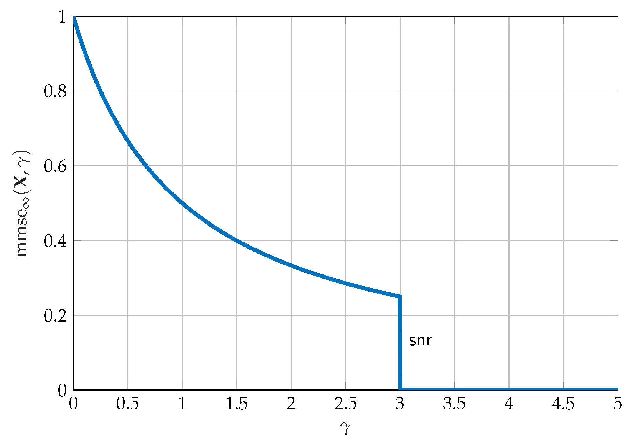
Figure 4.
Wiretap Channels. (a) The Wiretap Channel; (b) The Gaussian Wiretap Channel.
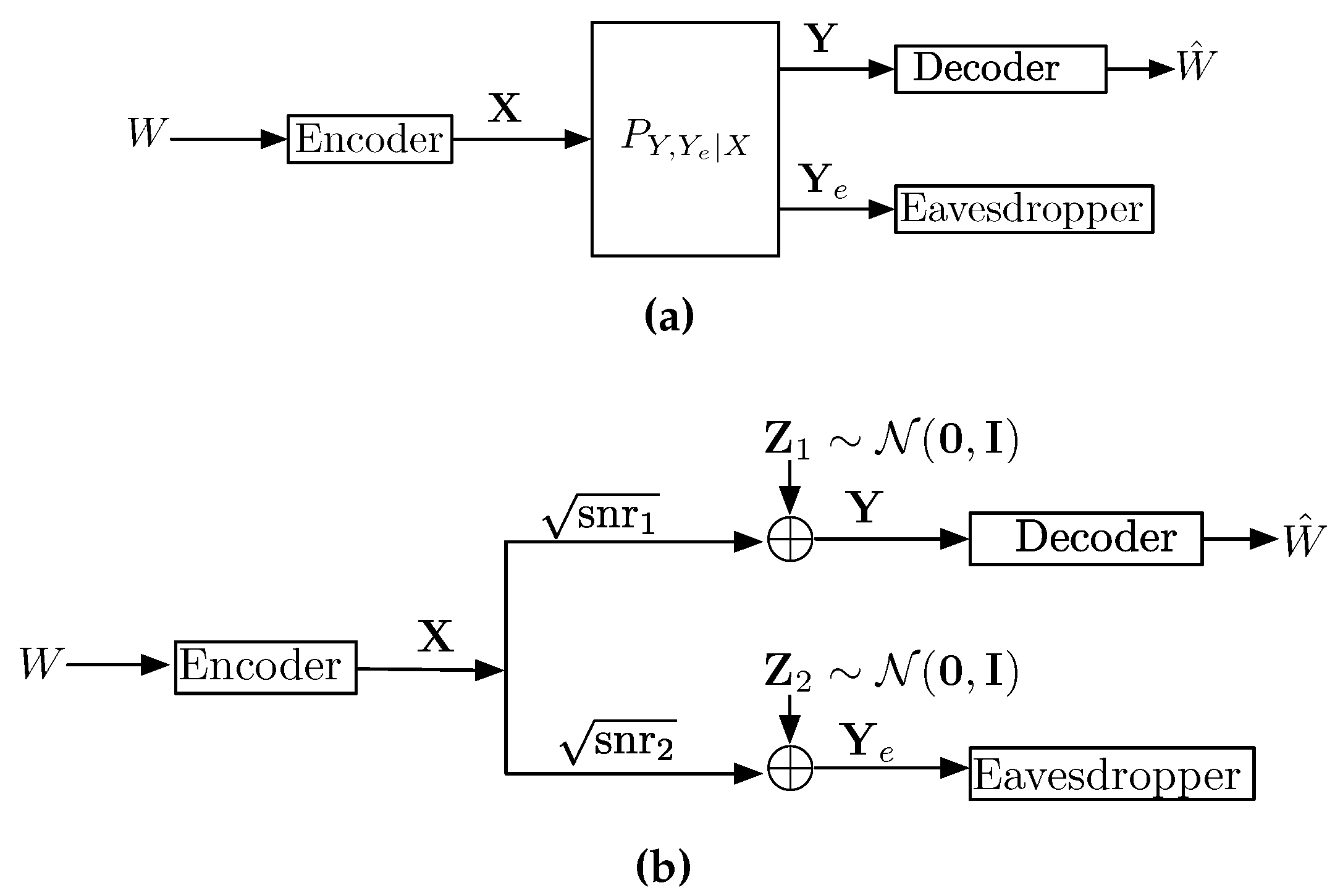
Figure 5.
The above figure depicts the behavior of as a function of assuming (in dotted blue), the behavior assuming complete secrecy (in dashed red) and the behavior of for some arbitrary code of rate above secrecy capacity and below point-to-point capacity (in dash-dot black). We mark twice the rate as the area between and (in magenta). Parameters are and .
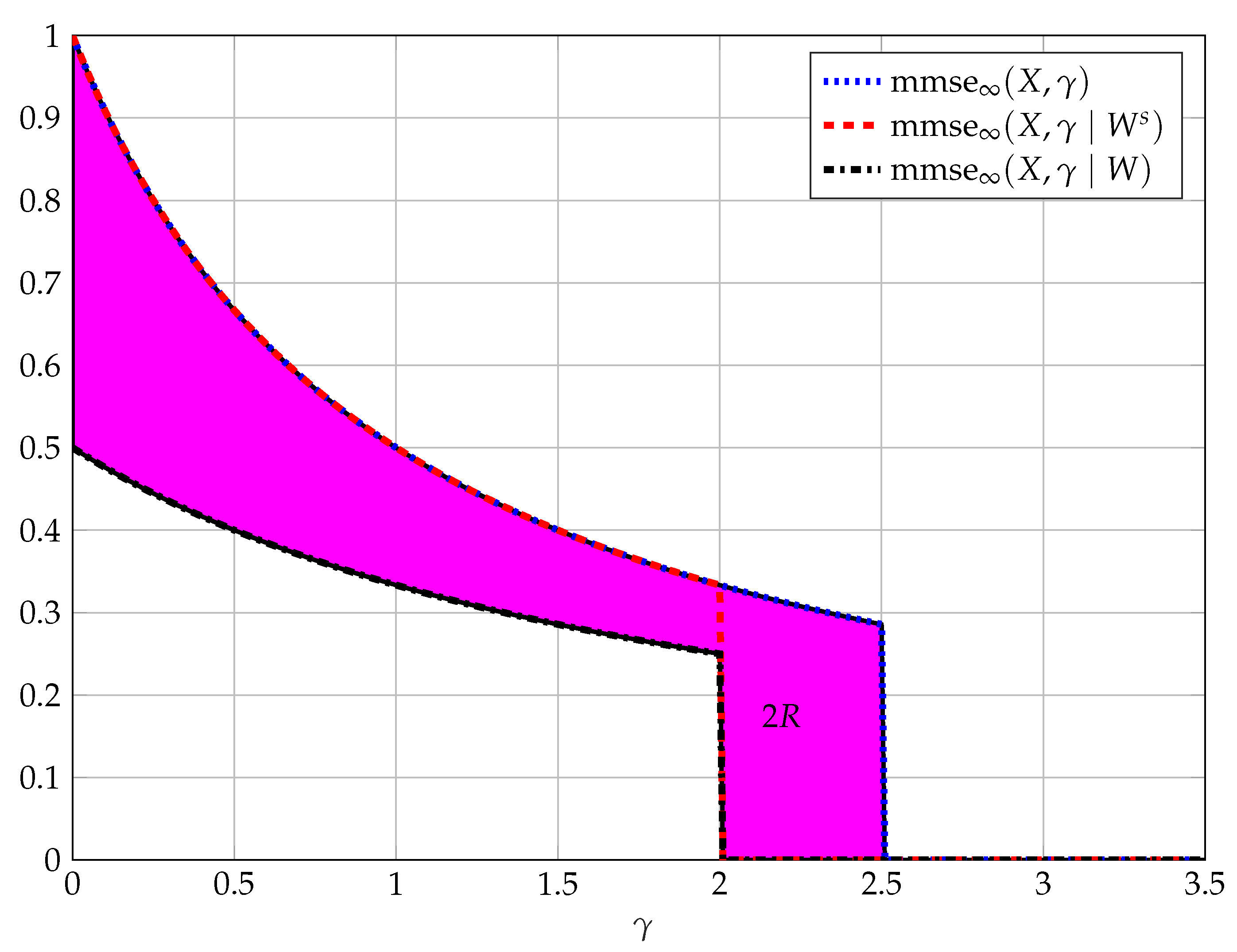
Figure 6.
Channels with disturbance constraints. (a) A point-to-point channel with a disturbance constraint; (b) A Gaussian point-to-point channel with the disturbance constraint.
Figure 6.
Channels with disturbance constraints. (a) A point-to-point channel with a disturbance constraint; (b) A Gaussian point-to-point channel with the disturbance constraint.

Figure 7.
Plot of vs. in dB, for , dB.

Figure 8.
Upper bounds on vs. . (a) For and . Here ; (b) For and . Several values of n.
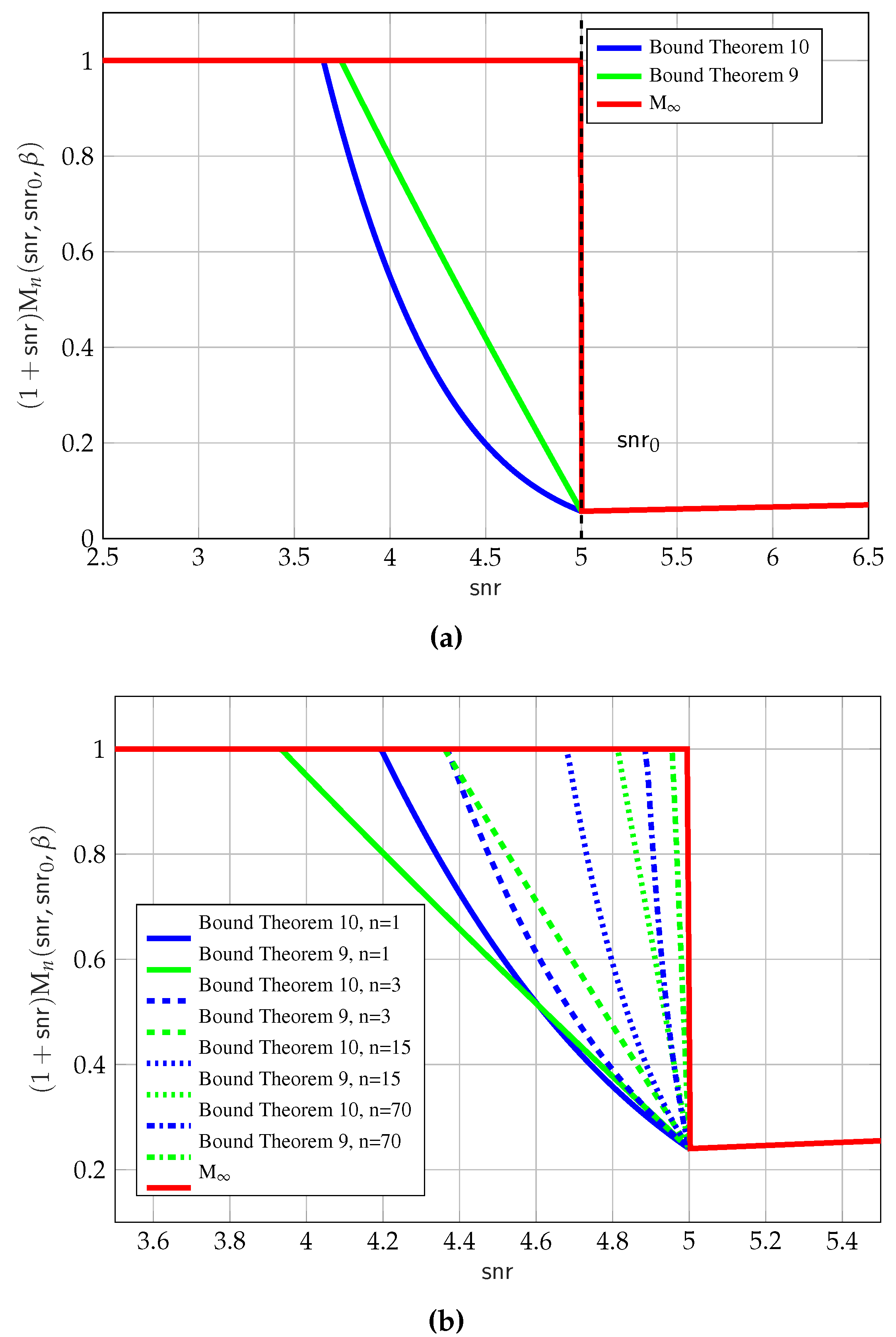
Figure 9.
Upper and lower bounds on vs. , for , .

Figure 10.
Upper and lower bounds on vs. , for and dB.

Figure 11.
Two-receiver broadcast channel. (a) A general BC; (b) A Gaussian BC.
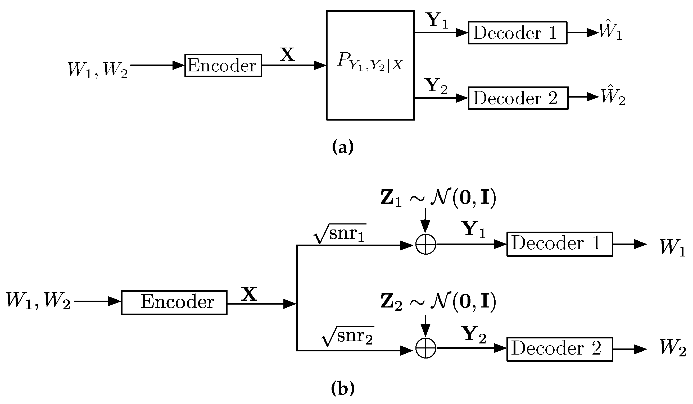
Figure 12.
In the above figure we consider the SNR-evolution of (in dashed blue) and (in solid red) required from an asymptotically capacity achieving code sequence for the Gaussian BC (rate on the boundary of the capacity region). Twice is marked as the area between these two functions (in magenta). The parameters are , , and .

Figure 13.
The above figure depicts a general transmission of independent messages, each required to be reliably decoded at the respective SNR . The rates are defined by the areas. (a) We observe that due to reliable decoding, the respective conditional MMSE converges to the MMSE; (b) we examine the same transmission as in (a), however here we observe the respective rates. The rates are defined by the areas. As an example we mark - twice the rate of message . Similarly one can mark the other rates and .
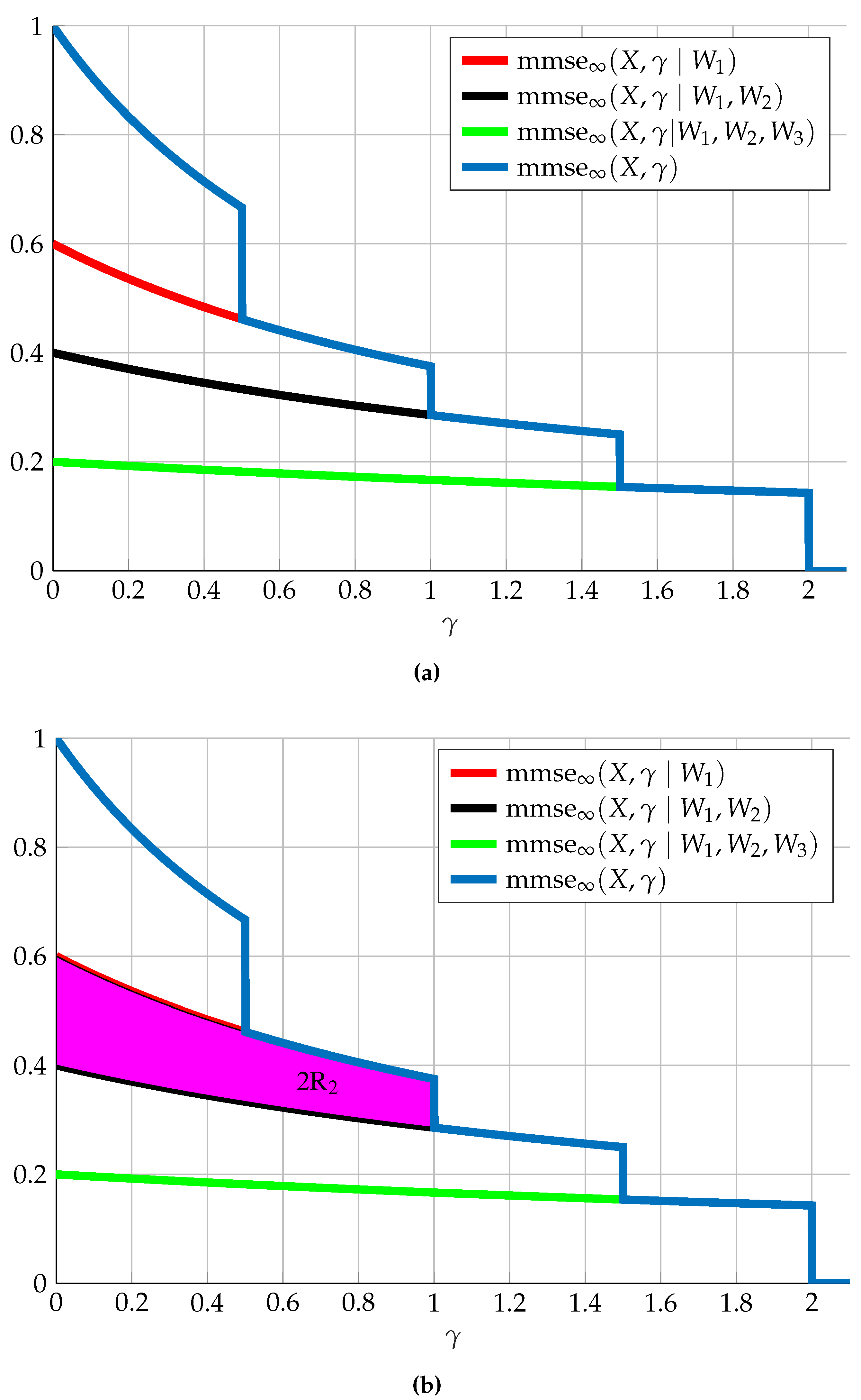
Figure 14.
The above figure depicts a general transmission of independent messages , each required to be reliably decoded at the respective SNR . Here we denote two equivocation measures and according to Theorem 15.
Figure 14.
The above figure depicts a general transmission of independent messages , each required to be reliably decoded at the respective SNR . Here we denote two equivocation measures and according to Theorem 15.
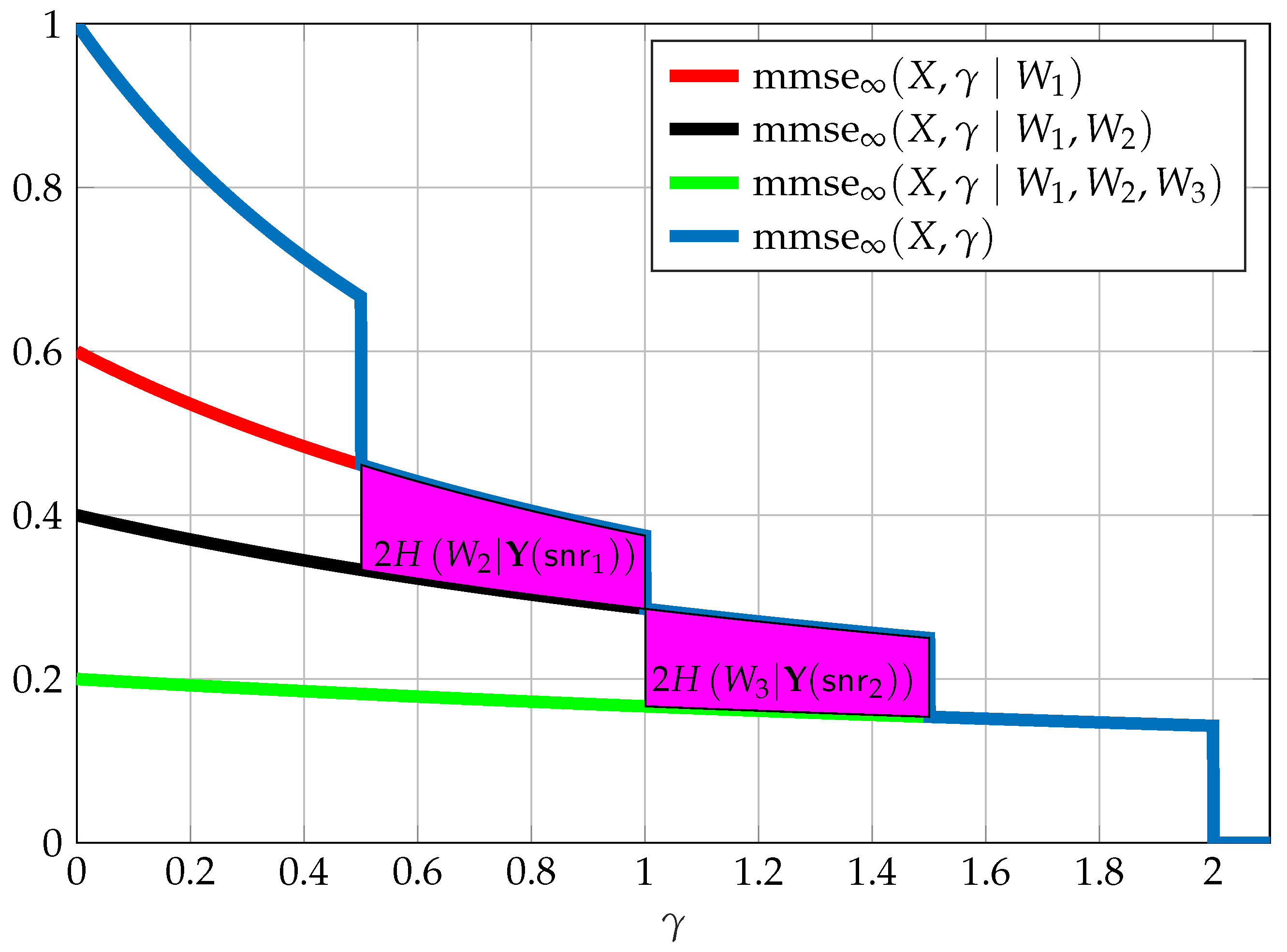
Figure 15.
Two user interference channels. (a) A general interference channel; (b) The Gaussian interference channel.
Figure 15.
Two user interference channels. (a) A general interference channel; (b) The Gaussian interference channel.

Figure 16.
gDoF of the G-IC.
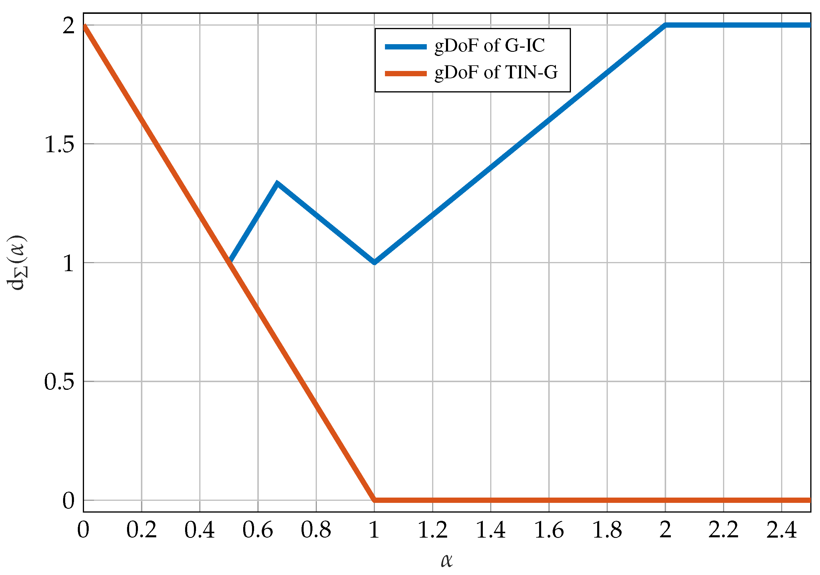

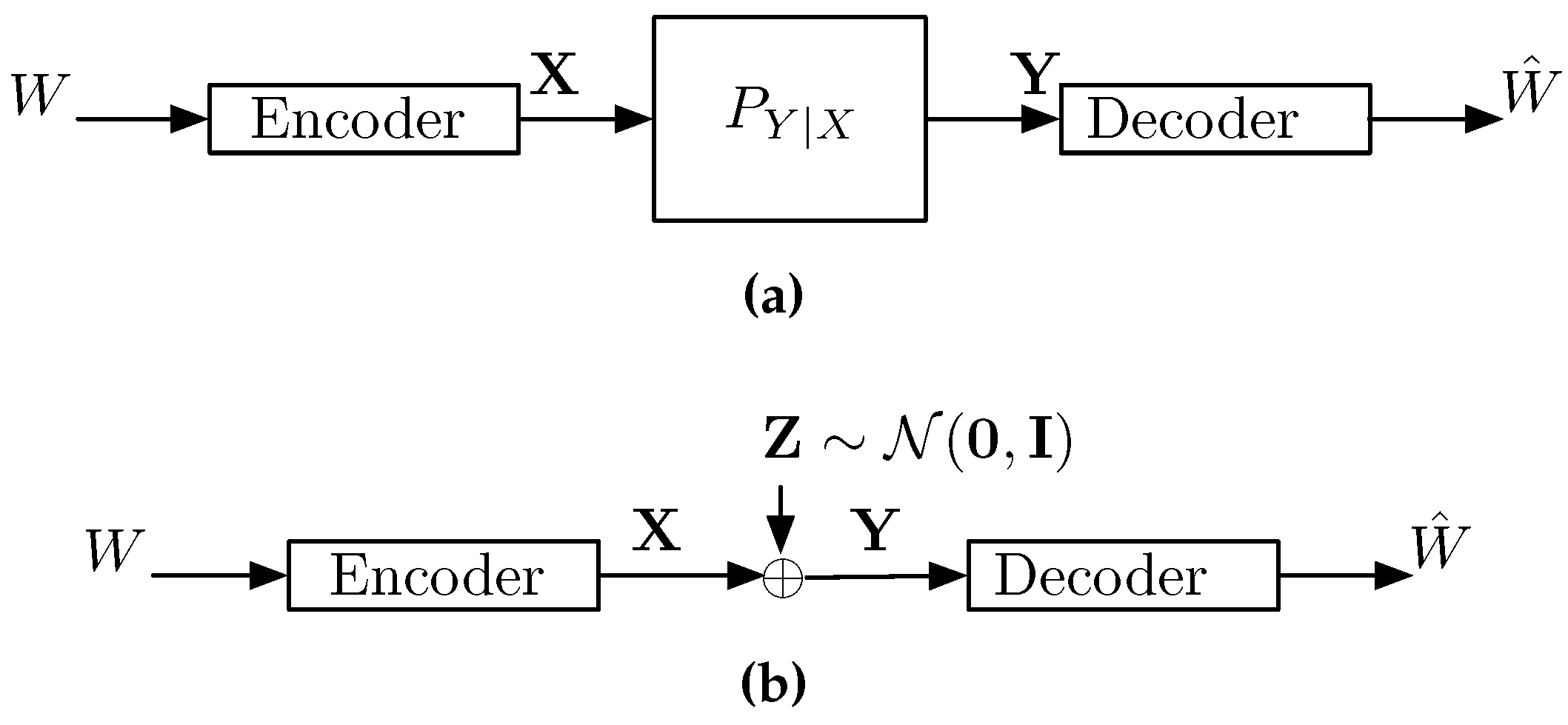
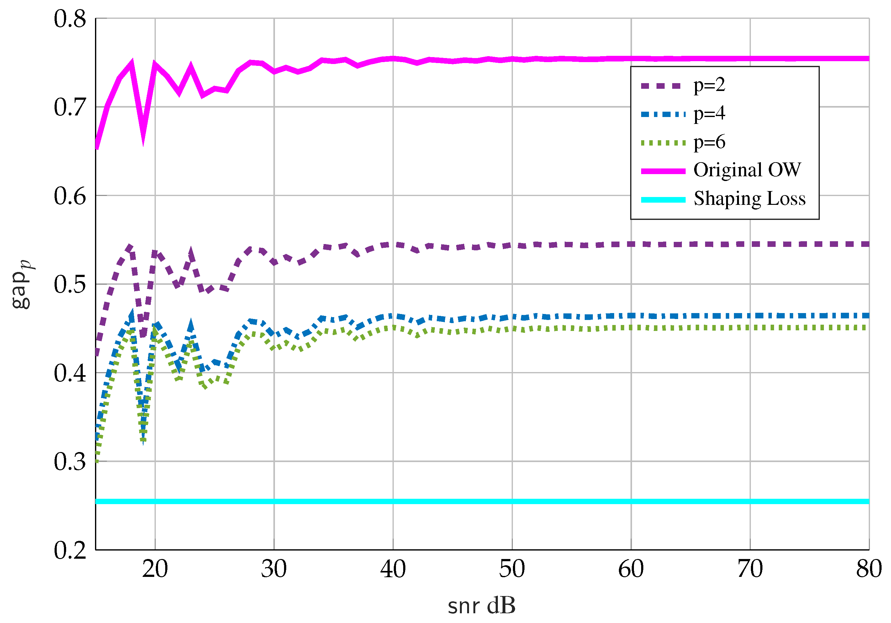
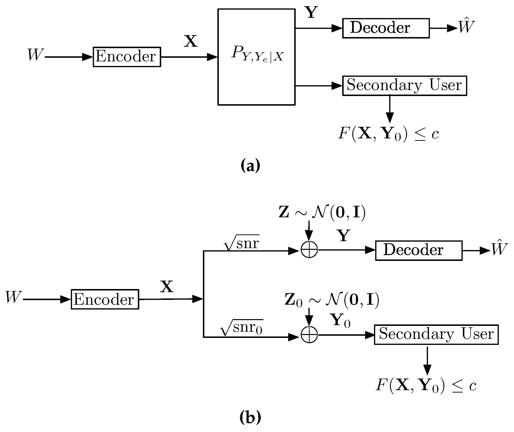
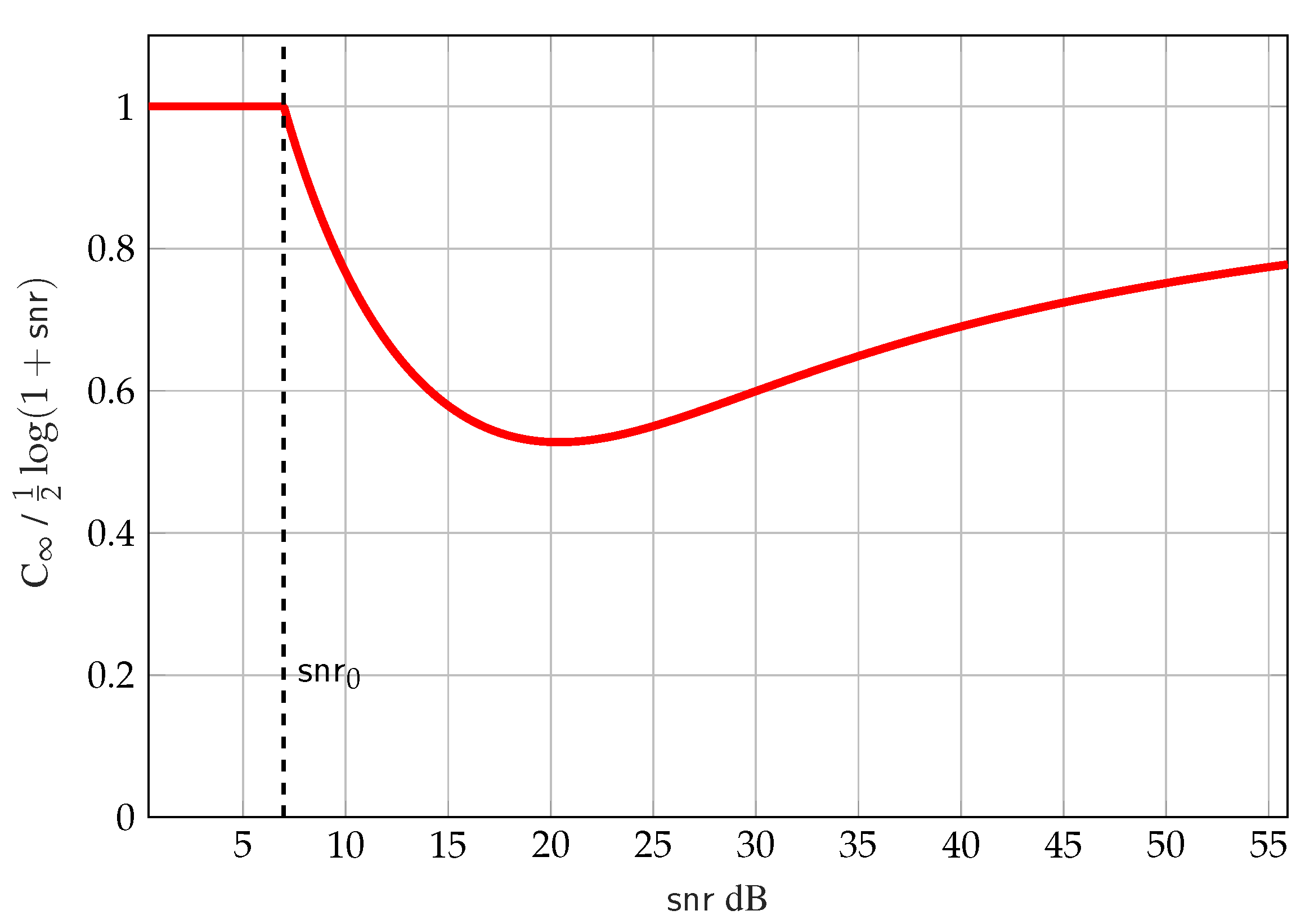
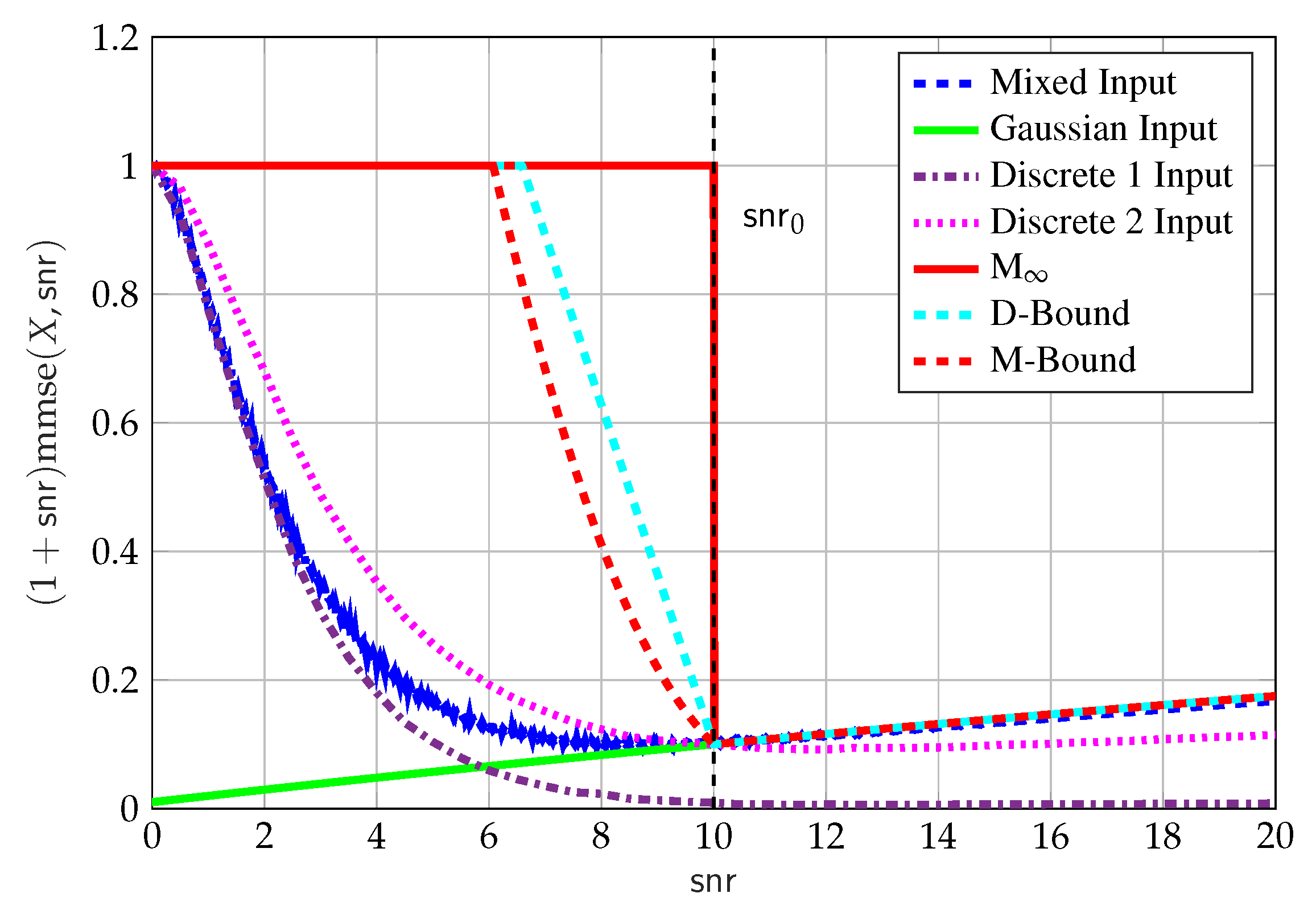
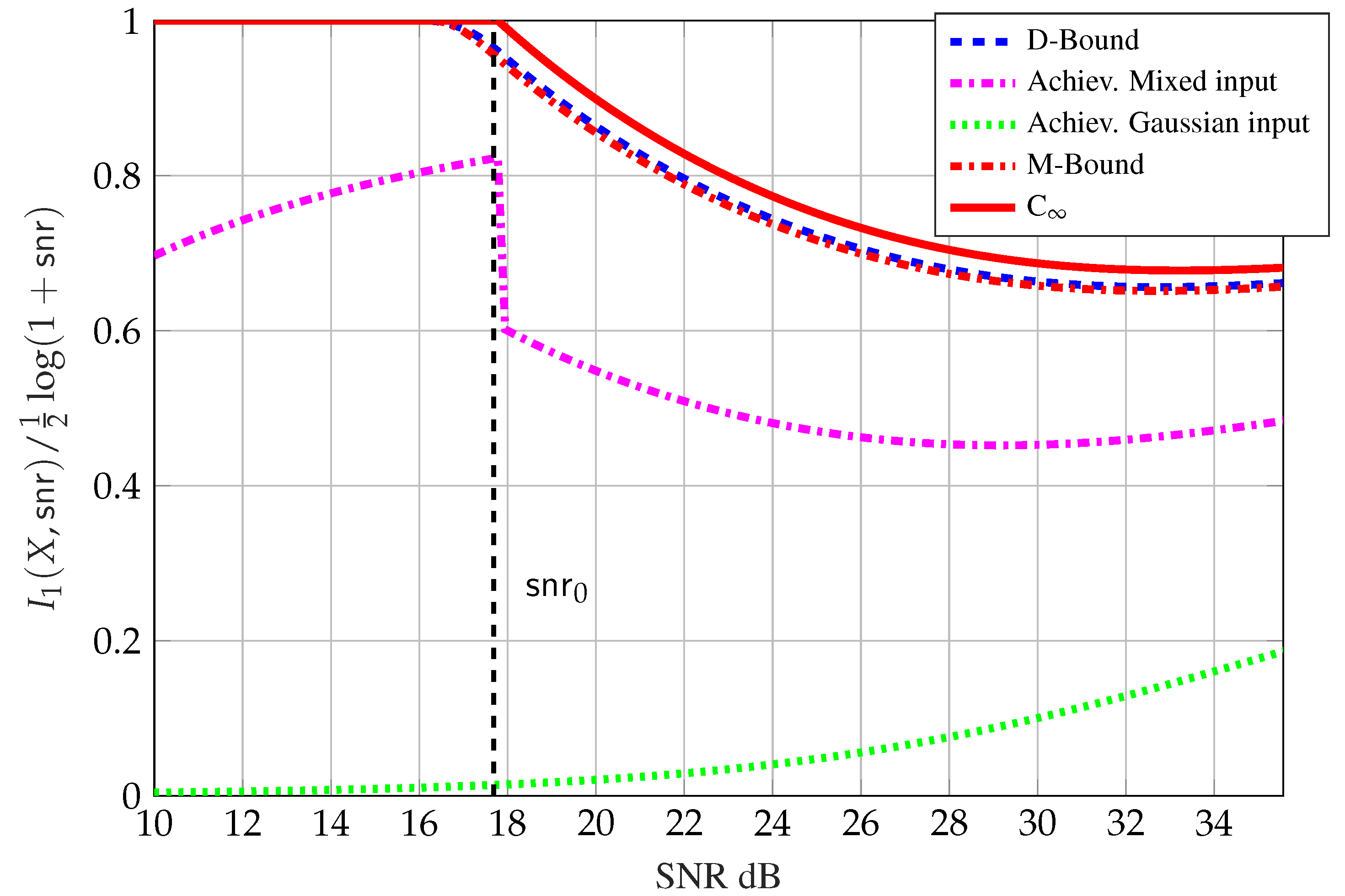
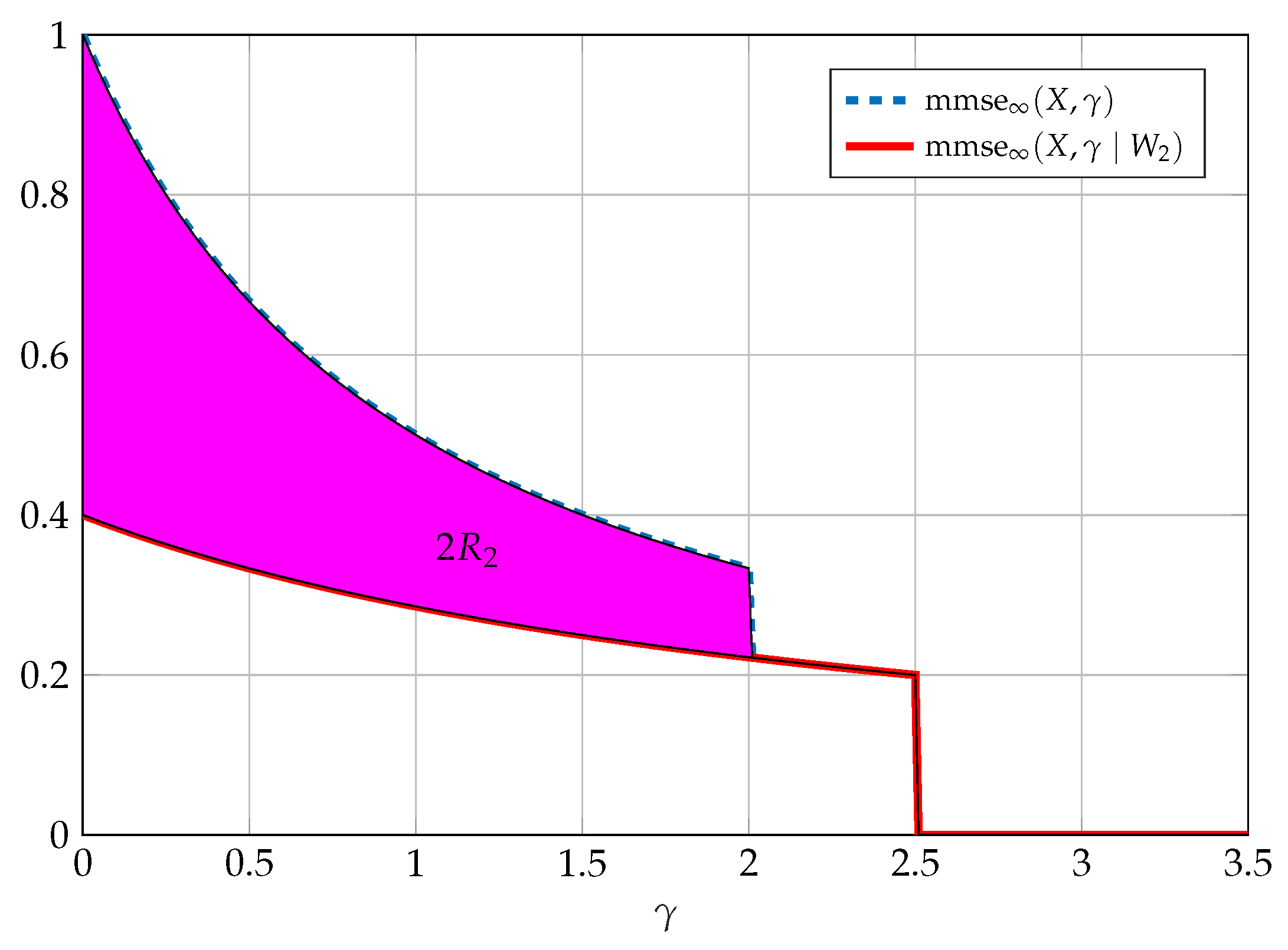
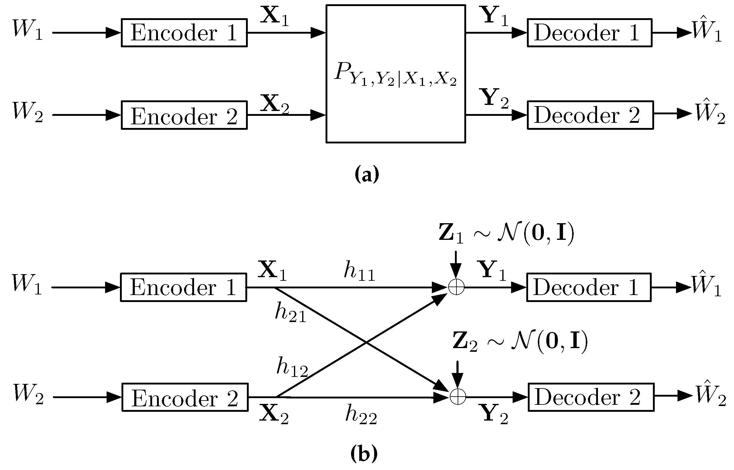
Table 1.
Parameters of the mixed input in (71) used in the proof of Proposition 11.
| Regime | Input Parameters |
|---|---|
| Weak Interference () | , |
| Strong Interference () | , , |
© 2017 by the authors. Licensee MDPI, Basel, Switzerland. This article is an open access article distributed under the terms and conditions of the Creative Commons Attribution (CC BY) license (http://creativecommons.org/licenses/by/4.0/).
Share and Cite
MDPI and ACS Style
Dytso, A.; Bustin, R.; Poor, H.V.; Shamai, S. A View of Information-Estimation Relations in Gaussian Networks. Entropy 2017, 19, 409. https://doi.org/10.3390/e19080409
AMA Style
Dytso A, Bustin R, Poor HV, Shamai S. A View of Information-Estimation Relations in Gaussian Networks. Entropy. 2017; 19(8):409. https://doi.org/10.3390/e19080409
Chicago/Turabian StyleDytso, Alex, Ronit Bustin, H. Vincent Poor, and Shlomo Shamai (Shitz). 2017. "A View of Information-Estimation Relations in Gaussian Networks" Entropy 19, no. 8: 409. https://doi.org/10.3390/e19080409
Note that from the first issue of 2016, this journal uses article numbers instead of page numbers. See further details here.