Effect of Slip Conditions and Entropy Generation Analysis with an Effective Prandtl Number Model on a Nanofluid Flow through a Stretching Sheet

1
Department of Civil Engineering, University of Birmingham, Edjbaston, Birmingham B15 2TT, UK
2
Department of Computer Science, Karakoram International University, Skardu Campus, Gilgit Baltistan 16100, Pakistan
*
Author to whom correspondence should be addressed.
Entropy 2017, 19(8), 414; https://doi.org/10.3390/e19080414
Submission received: 14 July 2017
/
Revised: 8 August 2017
/
Accepted: 9 August 2017
/
Published: 11 August 2017
(This article belongs to the Special Issue Entropy Generation in Nanofluid Flows)
Abstract
:This article describes the impact of slip conditions on nanofluid flow through a stretching sheet. Nanofluids are very helpful to enhance the convective heat transfer in a boundary layer flow. Prandtl number also play a major role in controlling the thermal and momentum boundary layers. For this purpose, we have considered a model for effective Prandtl number which is borrowed by means of experimental analysis on a nano boundary layer, steady, two-dimensional incompressible flow through a stretching sheet. We have considered γAl2O3-H2O and Al2O3-C2H6O2 nanoparticles for the governing flow problem. An entropy generation analysis is also presented with the help of the second law of thermodynamics. A numerical technique known as Successive Taylor Series Linearization Method (STSLM) is used to solve the obtained governing nonlinear boundary layer equations. The numerical and graphical results are discussed for two cases i.e., (i) effective Prandtl number and (ii) without effective Prandtl number. From graphical results, it is observed that the velocity profile and temperature profile increases in the absence of effective Prandtl number while both expressions become larger in the presence of Prandtl number. Further, numerical comparison has been presented with previously published results to validate the current methodology and results.
1. Introduction
Motivated scientists and researchers have identified the present age as an industrial and technological era. Thus, several theoretical and experimental studies have been undertaken to enhance the performance of industrial production methods. Researchers have identified that heat transfer is essential for the excellence of large scale processes. Usually, thermal characteristics are attained through conventional fluids but limited heat transfer capabilities have imposed a restriction on their utilization. Therefore, engineers thought that improved heat transfer routines should be implemented in order to achieve the desired outputs. For this purpose, they have performed several hypothetical and thought-provoking studies. Finally, they came up with the notion that the thermal ability of a carrier fluid can be improved with the escalation of its thermal conductance. Consequently, the idea of introducing particles into the basic fluid to provide a better transfer medium was introduced. The dimensions of these supplementary nanoparticles have attracted substantial interest due to their distinctive physical and chemical features. Now, it is well-established fact that the inclusion of nanomaterials enhances the thermal performance and conductivity of ordinary fluids. Thus, the dynamics of convective heat transport phenomenon via nanoparticles has grasped the focus of enthusiastic workers due to their incredible and extensive demand.
Choi [1] was the first to mention the idea of nanofluids. He defined nano liquids as an engineered dispersion of nanoparticles in a carrier fluid. He proved through experiments that the thermal capability of the host liquid is boosted with the addition of these small-sized materials. Masuda et al. [2] estimated the disparities in both thermal conductivity and the viscosity of conventional fluids by the dispersal of ultrafine particles in the host fluid. He reconfirmed that thermal transport in ordinary fluids increases tremendously with the suspension of ultrafine structures. Buongiorno [3] did seminal work on nanofluids by presenting a speculative model in order to interrogate the thermal features of carrier fluids. He contemplated that the improvement in conductance of regular fluid is due to the low volume fraction and small size of added nanoelements. Actually, nanotechnology is of great significance in numerous fields, including transportation, metallurgical and chemical devices, manufacturing of microscale objects, generation of power, cancer therapy, etc. The investigation on nanofluid flow over linearly stretched sheets was primarily initiated by Khan and Pop [4]. They numerically investigated the impact of the thermophoretic force and Brownian movement of nanostructures on thermal conductivity of the fluid. MHD stagnation boundary layer flow with collaborated effects of convective mode of heating, Brownian movement and thermophoretic force overstretched sheet were probed by Makinde et al. [5]. Nadeem et al. [6] performed numerical analysis of the magnetohydrodynamic flow of Maxwell fluids past a stretching sheet in the presence of nanoparticles. Malik et al. [7] performed a computational study to explore the effects of nanoparticles on an Eyring-Powel fluid model. Raju and Sandeep [8] addressed thermal and concentration transport due to Casson nanofluids in a rotating frame. Saleem and Nadeem [9] performed a comprehensive homotopy analysis to anticipate the impact of higher grade nanofluids over a rotatory cone. Raju et al. [10] conducted a comparative study to evaluate the fabulous enhancement in host fluid properties considering various types of metallic nanostructures. He also depicted the collaborative effects of temperature-dependent viscosity. A few recent studies exploring the the characteristics of nanofluids may be found in [11,12,13,14,15].
New resources to improve the heat transfer properties are becoming very important in many industrial applications. The study of heat transfer is not limited to an industrial application but also in much other applications such as wire drawing, metal spinning aerodynamics extrusion of plastic sheets and hot rolling. Utilization of solid nanoscale particles in working liquids is considered one of the most advanced techniques for improving their heat transfer characteristics. Several investigations have been made the effect of heat transfer in a nanofluid. Radiative heat transfer of nanofluids with variant surface heat flux and the effects of chemically reacting species were demonstrated by Zhang et al. [16]. Nield and Kuznetsov [17] capitalized on the Buongiorno model to adumbrate convective heat transfer induced by vertically stretched surfaces immersed in a Darcy medium. They reported that the strength of the heat transfer rate decreases by escalating the Brownian motion and thermophoresis parameters. The collective heat and mass features over a permeable exponentially stretched surface with second order slip were discussed by Rahman et al. [18]. Bhatti et al. [19] examined the numerical simulation of fluid flow over a shrinking sheet with heat transfer. Moreover, some more investigations of heat transfer with different geometries such as stretching sheet can be viewed in [20,21,22,23,24].
In 1996 Bejan [25] employed the second law of thermodynamics by means of entropy generation minimization. He covered the entropy generation minimization, particularly in the field of storage, heat transfer, thermal science and thermal power conversion. The thermodynamics approach plays a vital role in optimizing thermal engineering devices for higher energy efficiency. For this purpose, the minimization of entropy generation is used to determine the level of the available irreversibility in a process. These discussions clearly indicate that second law of thermodynamics is more reliable than the first law to determine the efficiency in the heat transfer system. Much more attention needs to be paid to optimize the heat transfer in electronic devices and engineering systems. Abbas et al. [26] studied the minimization of entropy generation of the peristaltic flow of nanofluid by using an analytical technique. Entropy generation of a Casson nanofluid over a stretching sheet has been analyzed by Abolbashari et al. [27]. For further works about entropy generation of nanofluids, one can refer to [28,29,30,31,32].
At present, not much work has been mentioned about entropy generation of nanofluids over a stretching sheet in the presence of slip effects. With all this in mind, the aim of the current work was to analyze the impact of entropy generation in the presence of Prandtl number and slip conditions through a stretching sheet.
2. Mathematical Formulation
Let us consider a two-dimensional steady irrotational, incompressible γAl2O3-H2O and Al2O3-C2H6O2 nanofluid flow through a vertical stretching surface coinciding with a plane at . To derive the governing equations, Cartesian coordinates system has been taken with the x-axis considered as vertically upward. The nanofluid flow occurs due to a stretching of a sheet caused by a pair of opposite and equal forces along the x-axis. The stretching sheet velocity can be written as and the temperature at a stretching sheet is Where is the ambient temperature, a and b are constants. The governing equations for the heat transfer for a nanofluid and steady boundary layer convective flow can be described as [19]:
Their respective boundary conditions are given by:
3. Thermophysical Properties of γAl2O3-H2O and Al2O3-C2H6O2 Nanofluids
The heat capacitance , the effective dynamic viscosity and the coefficient of thermal expansion of a nanofluid are described as:
where, the nanofluid volume fraction in solid form is denoted as .
- (i)
- Dynamic viscosity model:
- (ii)
- Effective thermal conductivity model:
- (iii)
- Effective Prandtl number model:
To compute the specific heat for nanofluids and the density, Equation (4) is derived for this purpose. In Equations (5) and (6), the expression for a dynamic viscosity of nanofluid is obtained by means of least-squares curve fitting of a few scarce experimental results that can be viewed for considered mixtures [33,34]. Equations (7) and (8) are presented from a model presented by Hamilton and Crosser [35], associated the nanofluids thermal conductivity, however, the similar case also exists for γAl2O3 nanofluids [36]. Equations (9) and (10) describe the effective Prandtl number for γAl2O3 nanofluids which are obtained with the help of a curve fitting by means of regression laws [37].
By introducing the similarity variables as:
Using these transformations in Equations (2) and (3), we get:
where:
and is a mixed convection parameter.
The new form of the boundary conditions as:
where slip parameter .
It is worth mentioning that from Equations (15) and (16) the effective Prandtl number for γAl2O3-H2O and γAl2O3-C2H6O2 respectively, can be deduced. Similarly, the effective Prandtl number is mentioned in Equations (17) and (18) for γAl2O3-H2O and γAl2O3-C2H6O2 respectively.
4. Important Physical Quantities
In the current study, the two most important physical quantities for the flow problem are the Nusselt number and skin friction coefficient which can be described as:
the dimensionless form of the skin friction coefficient defined as:
where is a local Reynolds number and it depends upon the stretching velocity and is the skin friction coefficient. The Nusselt number is defined as:
Using Equations (11) and (23), we have:
5. Entropy Generation Analysis
In the above volumetric rate of entropy generation equation, the first term represents entropy generation caused by heat transfer along a finite temperature difference. However, the second term reveals the entropy generation occurs due to viscous dissipation. The dimensionless form of entropy generation Ng describes the ratio between the local volumetric entropy generation rate NG to a characteristic rate of entropy generation . The characteristic entropy generation rate is described as:
By taking the ratio of Equations (26) and (27) the entropy generation number can be written as:
Using Equations (11) and (26), we get:
where is dimensionless temperature difference while Br indicates Brinkmann number, defined as:
6. Numerical Method
To proceed with STSLM, let us consider:
In the above equation, is the unknown functions that can be solved iteratively using the linearized governing equations and consider the are known through the previous iteration.
Equations (12) and (13) can be written in the following form:
where:
for γAl2O3-H2O
for γAl2O3-C2H6O2.
Using Equations (32), (12) and (13), we have:
along with their following boundary conditions in Equation (19). To obtain the subsequent solution for , Equation (34) can be solved iteratively. For this purpose, the algorithm initiated with an initial guess and with the help of initial approximation. The ith-order approximation solution for can be written as:
To get the solution for Equation (35), Chebyshev spectral collocation method is used. It is worth to mentioned that the right-hand side of Equation (34) for various values of i and by using the previous iterations we can get the coefficient of each parameter. Chebyshev spectral collocation method consists on the Chebyshev interpolating polynomials as given by:
The interval for the above Chebyshev interpolating polynomials are given in the region [−1, 1]. For the implications of this method and to convert the physical infinite region into the finite region we have applied a domain truncation method from the infinite region to a finite region as i.e., , and this way the targeted solution can be achieved in the interval instead of This leads to the mapping:
It can be observed from Equation (37) that to invoke boundary conditions expressed at infinity, we used the scaling parameter “”. Gauss-Lobatto collocation points have applied to define the Chebyshev nodes in . With the help of interpolating polynomial at each collocation points and truncated Chebyshev series, the inspection of the variable is examined. The series obtained from truncated Chebyshev is given as:
where is the Chebyshev polynomials. The derivatives of the variables at collocation points can be written as:
In the above Equation (39) the terms and D are the order of differential matrix and Chebyshev spectral differentiation matrix, respectively. Using Equations (38) and (39) into Equation (34) we have:
where:
In the above equations, the terms t, and represent the transpose, diagonal matrix of size and identity matrix, respectively. The BC is employed by removing the last column and last row of and by removing the last rows of and Setting the last and first rows of and to be zero. The solution for are iteratively obtained after solving:
It is worth to mentioned also that after obtaining the solution from Equation (41), we can apply directly the Chebyshev pseudo-spectral method to Equation (14) we have:
With their relevant boundary conditions:
where is the set linear differential equations and is the corresponding boundary conditions and is a vector of zeros. The obtained boundary conditions from Equation (43) is followed by the first and last rows of and , respectively.
7. Results and Discussion
This section describes the numerical and graphical results against all the governing parameters involved in the present flow problem. To analyze the proposed technique named Successive Taylor Series Linearization Method (STSLM), we have presented a comparison with previously published results and it is seen that the present results are in excellent agreement, which ensures the validity of the present methodology. In this methodology, the appropriate number of collocation points is considered as while the suitable value of is considered to be . It is analyzed that the values of the parameters mentioned above are the best ever results as far as the current flow is concerned, moreover, the present findings are in excellent agreement with the published results. STSLM is computationally quite efficient and accurate in comparison with other numerical methods as it provides precise results prominently when a governing problem is directly solved. Table 1 represents the thermo-physical properties of alumina, ethylene glycol and water whereas Table 2 reveals the numerical comparison of with previously published results [44,45,46]. Table 3 shows skin friction coefficient for various values of Prandtl number and the numerical results of Nusselt number and mixed convection parameter. Figure 1, Figure 2, Figure 3, Figure 4, Figure 5, Figure 6, Figure 7, Figure 8, Figure 9 and Figure 10 are sketched for different values of Prandtl number slip parameter , volume fraction of nano particle , mixed convection parameter , Brinkmann number and Reynolds number Re etc. against velocity profile , temperature profile and entropy profile Ng.
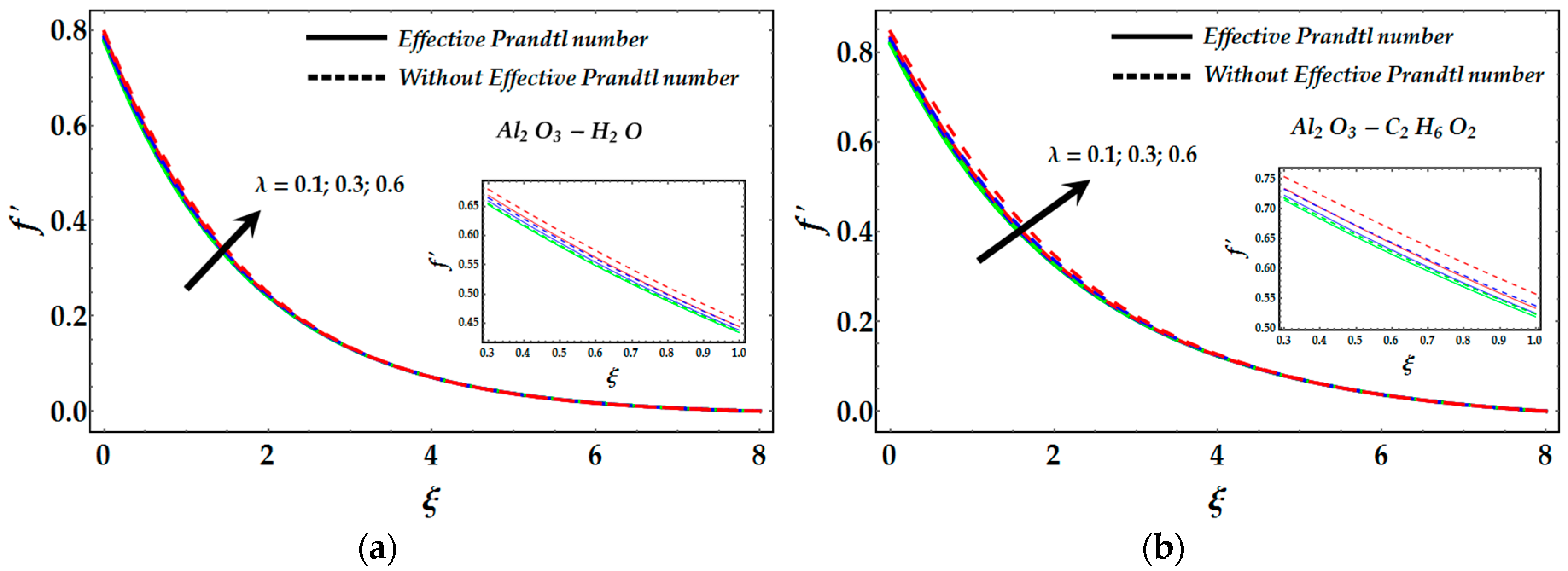
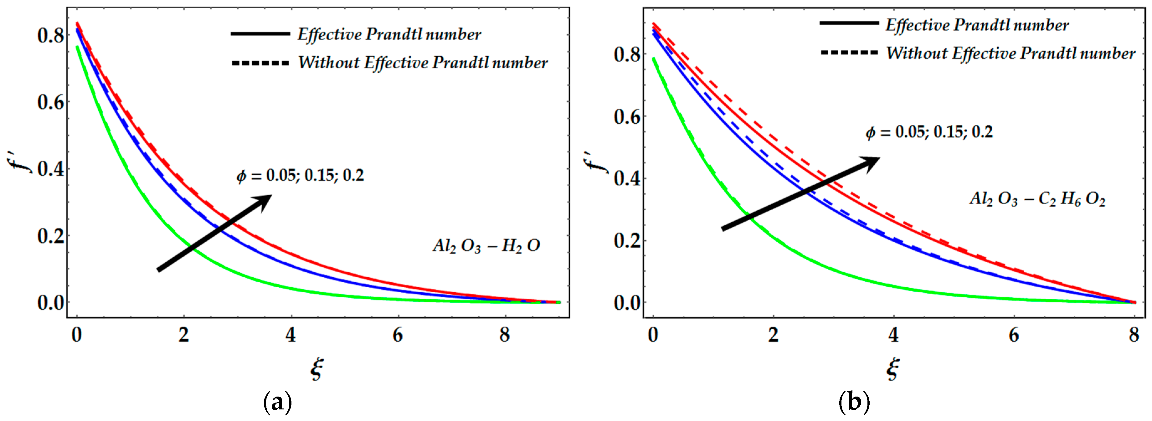
Figure 1, Figure 2 and Figure 3 are sketched for the velocity profiles against multiple values of the slip parameter , mixed convection parameter , and volume fraction of nanoparticles . It is observed in Figure 1 that the slip parameter significantly reduces the velocity profile for both γAl2O3-C2H6O2 and γAl2O3-H2O nanofluids. However, in the absence of an effective Prandtl number, the velocity profile rises. Figure 2 shows the variation of velocity against multiple values of the mixed convection parameter . In this figure, we can see that the mixed convection parameter does do not cause any major effect on γAl2O3-C2H6O2 and γAl2O3-H2O nanofluids. Mixed convection parameter enhances the velocity profile in the absence and presence of effective Prandtl number. Figure 3 depicts the effect of nanoparticle volume fraction on velocity. The results for single-phase flow can be reduced by taking in the governing equations.
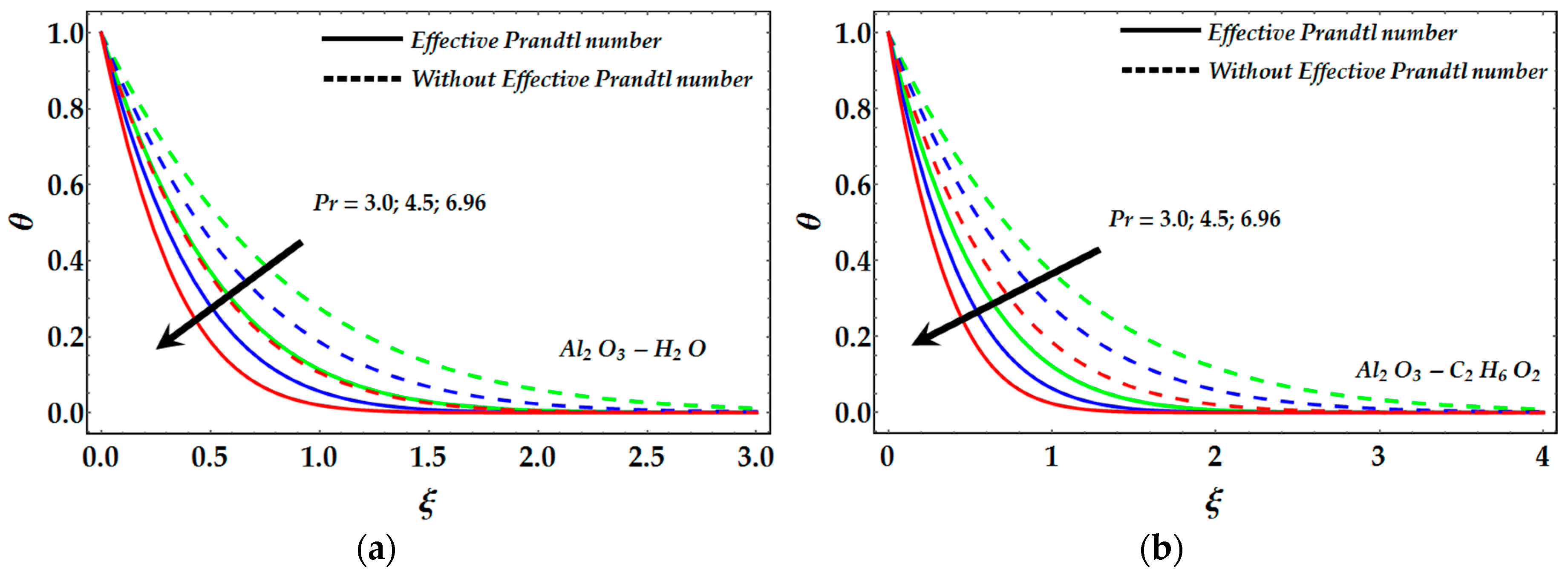
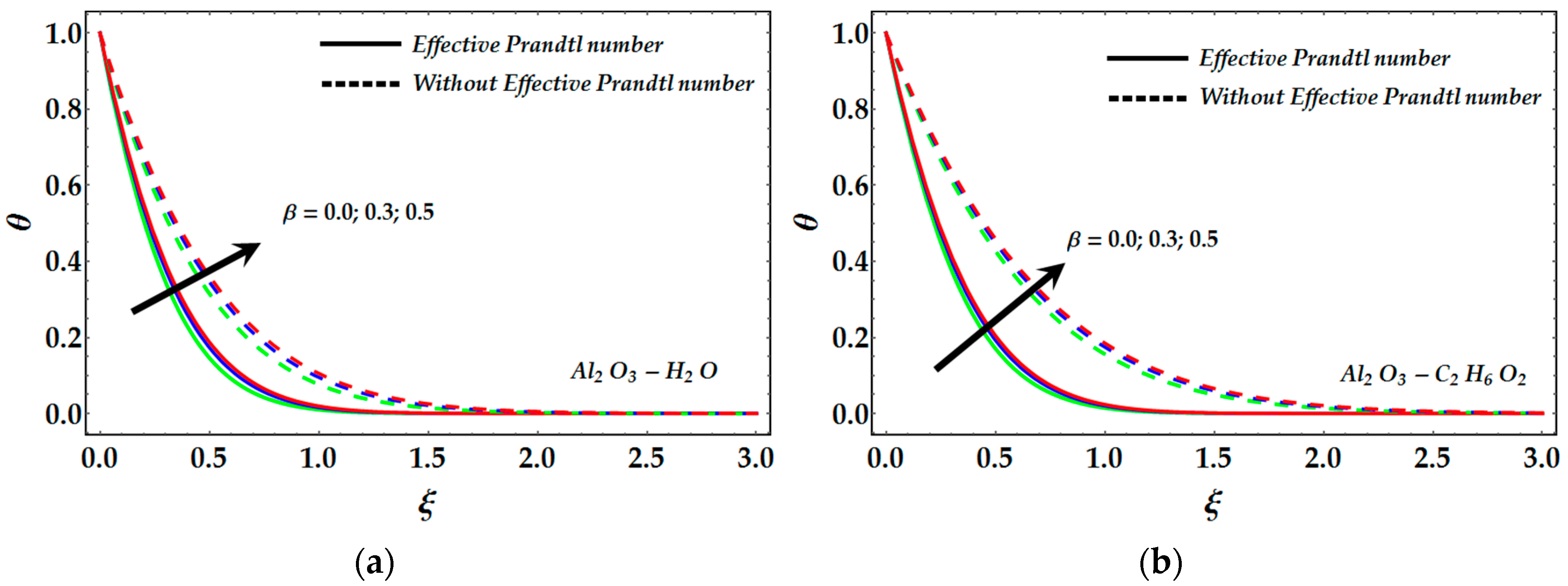
In these figures, we can see that the nanoparticle volume fraction significantly boost the velocity profiles, however, there is not significant effect of effective Prandtl number on γAl2O3-H2O fluid, whereas for γAl2O3-C2H6O2 fluid the effective Prandtl number tends to diminish the velocity more significantly as compared to γAl2O3-H2O fluid. Figure 4, Figure 5 and Figure 6 displayed the behavior of temperature profile against Prandtl number , Slip parameter , and nanoparticle volume fraction . Figure 4 depicts that reduction in temperature profile for both γAl2O3-C2H6O2 and γAl2O3-H2O nanofluids for larger values of Prandtl number . Prandtl number is helpful to control the relative thickness of the thermal and momentum boundary layers in heat transfer cases. The heat diffuses more rapidly as compared to velocity in the presence of a small Prandtl number. However, the greater impact of Prandtl number reveals that momentum diffusivity is more dominating over thermal diffusivity. Figure 5 is sketched for different values of slip parameter In this figure, we can see that the slip effects causes marked increment in the temperature profile for both γAl2O3-C2H6O2 and γAl2O3-H2O nanofluids. Figure 6 represents the variation of nanoparticle volume fraction on temperature profile. It can be viewed from Figure 6 that the temperature profiles for both γAl2O3-C2H6O2 and γAl2O3-H2O nanofluids increase when the Prandtl number does not exist, however, the behavior becomes quite the contrary in the presence of an effective Prandtl number. In Figure 4, Figure 5 and Figure 6 we find that the magnitude of the temperature profile is significantly lower in the presence of an effective Prandtl number.
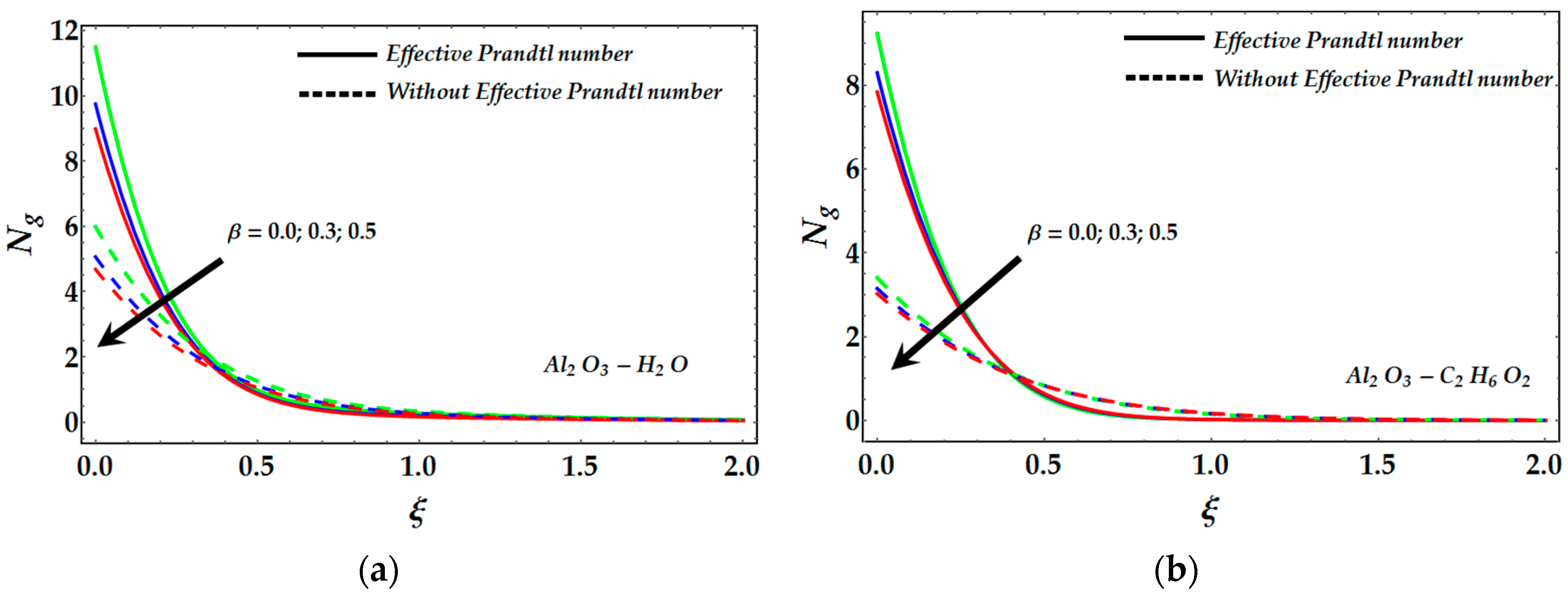
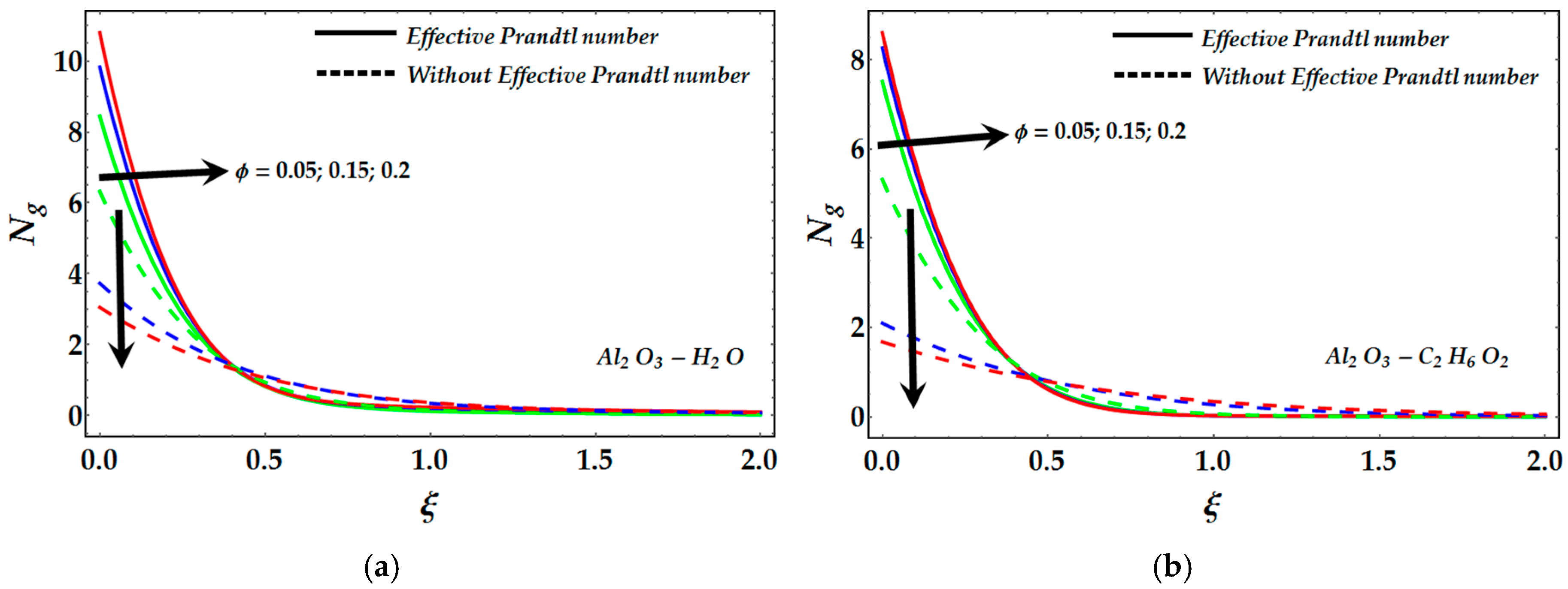
Figure 7, Figure 8, Figure 9 and Figure 10 elucidate the behavior of the entropy profile against the various values of slip parameter , volume fraction of nanoparticles , Brinkmann number Br and Reynolds number Re. It can be observed from Figure 7 that an increment in slip parameter , significantly enhances the entropy profile. However, it is found that in the presence of effective Prandtl number the entropy profile rises for γAl2O3-C2H6O2 and γAl2O3-H2O nanofluids. Figure 8 depicts that the entropy profile increases for higher values of the nanoparticle volume fraction in the presence of an effective Prandtl number whereas the behavior is contrary in the absence of an effective Prandtl number. An interesting thing observed here that in the absence of an effective Prandtl number, the entropy profile changes its behavior when for both γAl2O3-C2H6O2 and γAl2O3-H2O nanofluids.
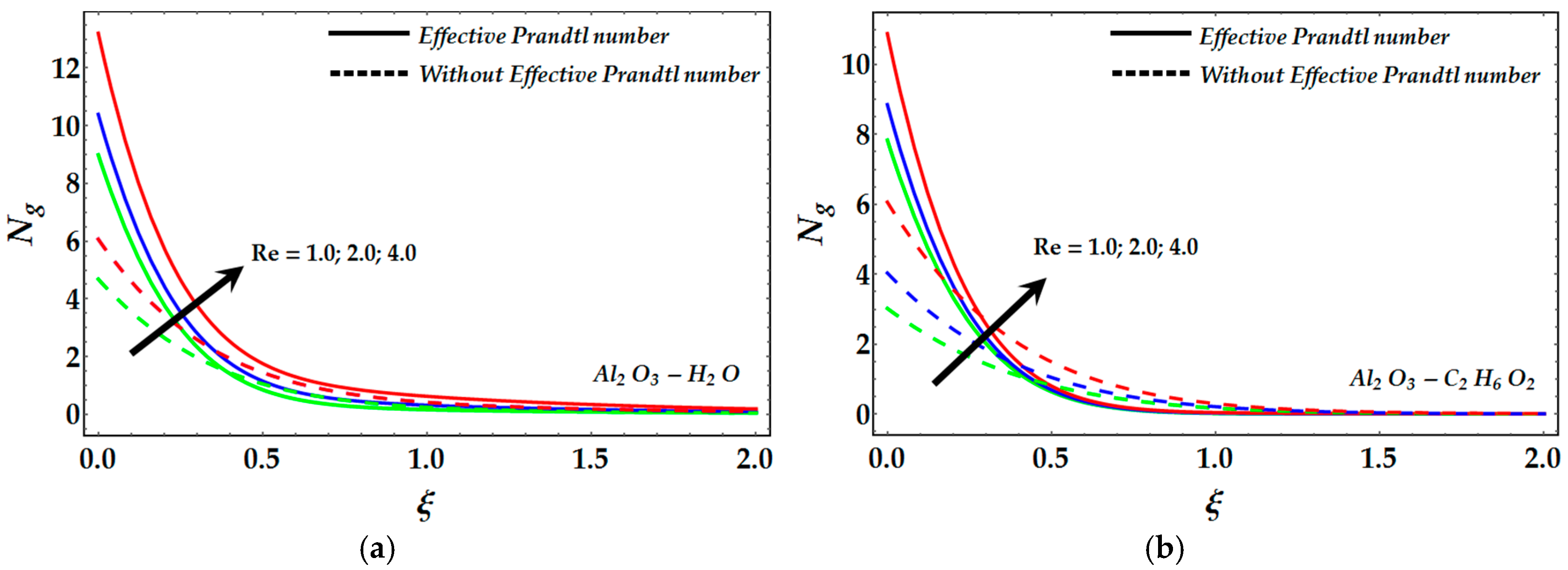
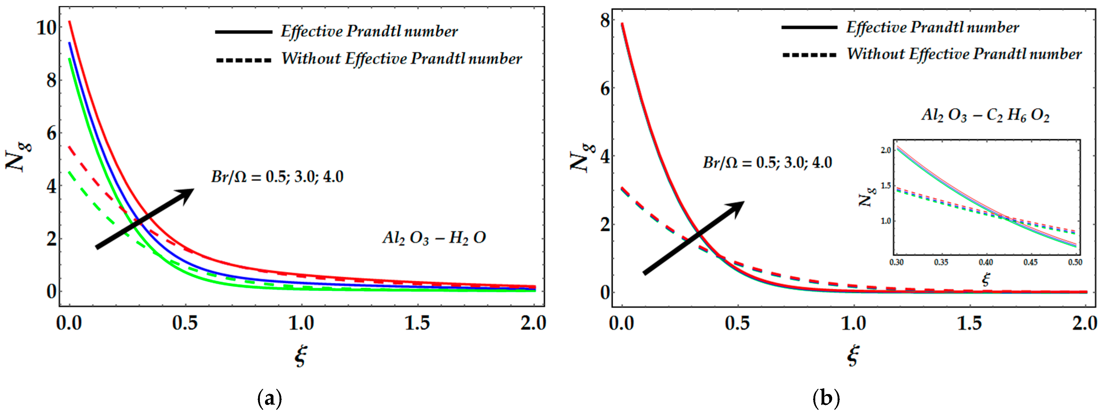
Figure 9 is sketched for different values of Brinkmann number Br and temperature difference . It is seen from this figure that the entropy profile increases for higher values of . However, for γAl2O3-C2H6O2 nanofluid, the variation in entropy profile is very small. Figure 10 shows that an increment in Reynolds number Re markedly enhances the entropy profile due to heat transfer in a boundary layer and nanofluid friction for both γAl2O3-C2H6O2 and γAl2O3-H2O nanofluids. An increment in Reynolds number causes a disturbance in the flow field and then chaos occurs in the movement of fluid. The presence of an effective Prandtl number enhances the entropy profile.
8. Conclusions
In this article, we have considered the slip effects on nanofluid flow through a stretching sheet in the absence and presence of an effective Prandtl number. A numerical technique (STSLM) with the combination of the Chebyshev spectral collocation method has been used to obtain the numerical solutions. A good numerical comparison with previously published results has been presented to validate the current methodology and results. The current investigation leads to the following important conclusions:
- An increment in nanoparticle volume fraction causes a marked increment in the velocity of nanofluids.
- Slip effects tend to provide a significant resistance in the velocity profile for both γAl2O3-C2H6O2 and γAl2O3-H2O nanofluids. The existence of Prandtl number tends to diminish the velocity profile.
- A remarkable reduction occurs in the temperature profile by increasing the Prandtl number for both γAl2O3-C2H6O2 and γAl2O3-H2O nanofluids.
- The impact of slip conditions significantly enhances the temperature profile in the presence and absence of an effective Prandtl number.
- The temperature profile is enhanced due to nanoparticle volume fraction in the absence of an effective Prandtl number, whereas the converse behavior is seen in the presence of an effective Prandtl number.
- Due to the increment in slip parameter the entropy profile decreases whereas an effective Prandtl number enhances entropy generation.
- Reynolds number and Brinkmann number also enhance the entropy profile and a similar relation has been observed in the presence of an effective Prandtl number.
Acknowledgments
We express our gratitude to anonymous referees for their constructive reviews of the muniscript and for helpful comments.
Author Contributions
Mohammad Mehdi Rashidi conceived and designed the mathematical formulation of the problem, whereas solution of the problem and graphical results is analyzed by Munawwar Ali Abbas. All authors have read and approved the final manuscript.
Conflicts of Interest
The authors declare no conflict of interest.
Nomenclature
| Temperature of wall | |
| Nanofluid, Prandtl number | |
| g,m/ | Gravity |
| Nanofluid, thermal conductivity | |
| Nanofluid temperature | |
| Base fluid Prandtl number | |
| Nusselt number of nano fluid | |
| skin friction coefficient | |
| Base fluid, thermal conductivity | |
| ambient temperature | |
| m/s | Expression of velocity in horizontal and vertical directions, Respectively |
| Nanoparticles, thermal conductivity |
Greek Symbols
| parameter of mixed convection | |
| volume fraction of the model | |
| nanofluid effective density | |
| viscosity of the nanofluid effective dynamic | |
| coefficient of Nanoparticles thermal expansion | |
| the base fluid dynamic viscosity | |
| Base fluid thermal expansion coefficient | |
| Nanoparticles density | |
| base fluid density | |
| nanofluid thermal expansion coefficient | |
| variable of space |
References
- Chol, S.U.S.; Eastman, J.A. Enhancing thermal conductivity of fluids with nanoparticles. ASME-Publications-Fed 1995, 231, 99–106. [Google Scholar]
- Masuda, H.; Ebata, A.; Teramae, K.; Hishinunma, N.; Ebata, Y. Alteration of thermal conductivity and viscosity of liquid by dispersing ultra-fine particles (dispersion of γ-Al2O3, SiO2 and TiO2 ultra-fine particles). Netsu Bussei 1993, 7, 227–233. (In Janpanese) [Google Scholar] [CrossRef]
- Buongiorno, J. Convective transport in nanofluids. J. Heat Transf. 2006, 128, 240–250. [Google Scholar] [CrossRef]
- Khan, W.A.; Pop, I. Boundary-layer flow of a nanofluid past a stretching sheet. Int. J. Heat Mass Transf. 2010, 53, 2477–2483. [Google Scholar] [CrossRef]
- Makinde, O.D.; Khan, W.A.; Khan, Z.H. Buoyancy effects on MHD stagnation point flow and heat transfer of a nanofluid past a convectively heated stretching/shrinking sheet. Int. J. Heat Mass Transf. 2013, 62, 526–533. [Google Scholar] [CrossRef]
- Nadeem, S.; Haq, R.; Khan, Z.H. Numerical study of MHD boundary layer flow of Maxwell fluid past a stretching sheet in the presence of nanoparticles. J. Taiwan Inst. Chem. Eng. 2014, 45, 121–126. [Google Scholar] [CrossRef]
- Malik, M.Y.; Khan, I.; Hussain, A.; Salahuddin, T. Mixed convection flow of MHD Eyring-Powell nanofluid over a streching sheet: A numerical study. AIP Adv. 2015, 5, 117–118. [Google Scholar] [CrossRef]
- Raju, C.S.K.; Sandeep, N. Unsteady Casson nano over a rotating cone in a rotating frame filled with ferrous nanoparticles: A numerical study. J. Magn. Magn. Mater. 2017, 421, 216–224. [Google Scholar] [CrossRef]
- Nadeem, S.; Saleem, S. Analytical study of third grade fluid over a rotating vertical cone in thepresence of nanoparticles. Int. J. Heat Mass Transf. 2015, 85, 1041–1048. [Google Scholar] [CrossRef]
- Raju, C.S.K.; Sandeep, N.; Malvandi, A. Free convective heat and mass transfer of MHD Non-Newtonian nanofluids over a cone in the presence of non-uniform heat soure/sink. J. Mol. Liq. 2016, 221, 108–115. [Google Scholar] [CrossRef]
- Nadeem, S.; Saleem, S. Unsteady mixed convection flow of nanofluid on a rotating cone with magnetic field. Appl. Nanosci. 2014, 4, 405–414. [Google Scholar] [CrossRef]
- Bhatti, M.M.; Rashidi, M.M. Effects of thermo-diffusion and thermal radiation on Williamson nanofluid over a porous shrinking/stretching sheet. J. Mol. Liq. 2016, 221, 567–573. [Google Scholar] [CrossRef]
- Nadeem, S.; Haq, R.; Khan, Z.H. Numerical solution of non-Newtonian nanofluid flow over a stretching sheet. Appl. Nanosci. 2014, 4, 625–631. [Google Scholar] [CrossRef]
- Hsiao, K.L. Combined electrical MHD heat transfer thermal extrusion system using Maxwell fluid with radiative and viscous dissipation effects. Appl. Therm. Eng. 2017, 112, 1281–1288. [Google Scholar] [CrossRef]
- Hsiao, K.L. To promote radiation electrical MHD activation energy thermal extrusion manufacturing system efficiency by using Carreau-Nanofluid with parameters control method. Energy 2017, 130, 486–499. [Google Scholar] [CrossRef]
- Zhang, C.; Zheng, L.; Zhang, X.; Chen, G. MHD flow and radiation heat transfer of nanofluids in porous media with variable surface heat flux and chemical reaction. Appl. Math. Model. 2015, 39, 161–184. [Google Scholar] [CrossRef]
- Nield, D.A.; Kuznetsov, A.V. The Cheng-Minkowycz problem for natural convective boundary-layer flow in a porous medium saturated by a nanofluid. Int. J. Heat Mass Transf. 2009, 52, 5792–5795. [Google Scholar] [CrossRef]
- Rahman, M.M.; Roşca, A.V.; Pop, I. Boundary layer flow of a nanofluid past a permeable exponentially shrinking/stretching surface with second order slip using Buongiorno’s model. Int. J. Heat Mass Transf. 2014, 77, 1133–1143. [Google Scholar] [CrossRef]
- Bhatti, M.M.; Shahid, A.; Rashidi, M.M. Numerical simulation of Fluid flow over a shrinking porous sheet by Successive linearization method. Alexandria Eng. J. 2016, 55, 51–56. [Google Scholar] [CrossRef]
- Hsiao, K.L. Stagnation electrical MHD nanofluid mixed convection with slip boundary on a stretching sheet. Appl. Therm. Eng. 2016, 98, 850–861. [Google Scholar] [CrossRef]
- Hsiao, K.L. Numerical solution for Ohmic Soret-Dufour heat and mass mixed convection of viscoelastic fluid over a stretching sheet with multimedia physical features. J. Aerosp. Eng. 2016, 30, 04016082. [Google Scholar] [CrossRef]
- Shahid, A.; Bhatti, M.M.; Bég, O.A.; Kadir, A. Numerical study of radiative Maxwell viscoelastic magnetized flow from a stretching permeable sheet with the Cattaneo–Christov heat flux model. Neural Comput. Appl. 2017. [Google Scholar] [CrossRef]
- Mishra, S.R.; Bhatti, M.M. Simultaneous effects of Chemical reaction and Ohmic heating with heat and mass transfer over a stretching surface: A numerical study. Chin. J. Chem. Eng. 2017. [Google Scholar] [CrossRef]
- Hsiao, K.L. Micropolar nanofluid flow with MHD and viscous dissipation effects towards a stretching sheet with multimedia feature. Int. J. Heat Mass Transf. 2017, 112, 983–990. [Google Scholar] [CrossRef]
- Bejan, A. Entropy generation minimization: The new thermodynamics of finite-size devices and finite-time processes. J. Appl. Phys. 1996, 79, 1191–1218. [Google Scholar] [CrossRef]
- Abbas, M.A.; Bai, Y.; Rashidi, M.M.; Bhatti, M.M. Analysis of entropy generation in the flow of peristaltic nanofluids in channels with compliant walls. Entropy 2016, 18, 90. [Google Scholar] [CrossRef]
- Abolbashari, M.H.; Freidoonimehr, N.; Nazari, F.; Rashidi, M.M. Analytical modeling of entropy generation for Casson nano-fluid flow induced by a stretching surface. Adv. Powder Technol. 2015, 26, 542–552. [Google Scholar] [CrossRef]
- Qing, J.; Bhatti, M.M.; Abbas, M.A.; Rashidi, M.M.; Ali, M.E.S. Entropy generation on MHD Casson nanofluid flow over a porous stretching/shrinking surface. Entropy 2006, 18, 123. [Google Scholar] [CrossRef]
- Bhatti, M.M.; Rashidi, M.M.; Pop, I. Entropy Generation with nonlinear heat and Mass transfer on MHD Boundary Layer over a Moving Surface using SLM. Nonlinear Eng. 2017, 6, 43–52. [Google Scholar] [CrossRef]
- Rashidi, M.M.; Bhatti, M.M.; Abbas, M.A.; Ali, M.E.S. Entropy generation on MHD blood flow of nanofluid due to peristaltic waves. Entropy 2016, 18, 117. [Google Scholar] [CrossRef]
- Rashidi, M.M.; Bagheri, S.; Momoniat, E.; Freidoonimehr, N. Entropy analysis of convective MHD flow of third grade non-Newtonian fluid over a stretching sheet. Ain Shams Eng. J. 2015. [Google Scholar] [CrossRef]
- Bhatti, M.M.; Abbas, T.; Rashidi, M.M. Entropy generation as a practical tool of optimisation for non-Newtonian nanofluid flow through a permeable stretching surface using SLM. J. Comput. Des. Eng. 2017, 4, 21–28. [Google Scholar] [CrossRef]
- Lee, S.; Choi, S.U.-S.; Li, S.; Eastman, J.A. Measuring thermal conductivity of fluids containing oxide nanoparticles. J. Heat Transf. 1999, 121, 280–289. [Google Scholar] [CrossRef]
- Wang, X.; Xu, X.; Choi, S.U.-S. Thermal conductivity of nanoparticles-fluid mixture. J. Thermophys. Heat Transf. 1999, 13, 474–480. [Google Scholar] [CrossRef]
- Hamilton, R.L.; Crosser, O.K. Thermal conductivity of heterogeneous two component systems. Ind. Eng. Chem. Fundam. 1962, 1, 187–191. [Google Scholar] [CrossRef]
- Maiga, S.E.B.; Nguyen, C.T.; Galanis, N.; Roy, G. Heat transfer behaviors of nanofluids in a uniformly heated tube. Superlattices Microstruct. 2004, 35, 543–557. [Google Scholar] [CrossRef]
- Pop, C.V.; Fohanno, S.; Polidori, G.; Nguyen, C.T. Analysis of laminar-to-turbulent threshold with water c Al2O3 and ethylene glycol-c Al2O3 nanofluids in free convection. In Proceedings of the 5th IASME/WSEAS International Conference on Heat Transfer, Thermal Engineering and Environment, Athens, Greece, 25–27 August 2017; p. 188. [Google Scholar]
- Bhatti, M.M.; Rashidi, M.M. Entropy generation with nonlinear thermal radiation in MHD boundary layer flow over a permeable shrinking/stretching sheet: Numerical solution. J. Nanofluids 2016, 5, 543–548. [Google Scholar] [CrossRef]
- Bhatti, M.M.; Abbas, T.; Rashidi, M.M. Numerical Study of Entropy Generation with Nonlinear Thermal Radiation on Magnetohydrodynamics non-Newtonian Nanofluid Through a Porous Shrinking Sheet. J. Magn. 2016, 21, 468–475. [Google Scholar] [CrossRef]
- Bhatti, M.M.; Rashidi, M.M. Numerical simulation of entropy generation on MHD nanofluid towards a stagnation point flow over a stretching surface. Int. J. Appl. Comput. Math. 2017, 3, 2275–2289. [Google Scholar] [CrossRef]
- Abbas, T.; Ayub, M.; Bhatti, M.M.; Rashidi, M.M.; Ali, M.E.S. Entropy generation on nanofluid flow through a horizontal Riga plate. Entropy 2016, 18, 223. [Google Scholar] [CrossRef]
- Bhatti, M.M.; Abbas, T.; Rashidi, M.M.; Ali, M.E.S.; Yang, Z. Entropy generation on MHD Eyring–Powell nanofluid through a permeable stretching surface. Entropy 2016, 18, 224. [Google Scholar] [CrossRef]
- Bhatti, M.M.; Abbas, T.; Rashidi, M.M.; Ali, M.E.S. Numerical simulation of entropy generation with thermal radiation on MHD Carreau nanofluid towards a shrinking sheet. Entropy 2016, 18, 200. [Google Scholar] [CrossRef]
- Ali, M.E. Heat transfer characteristics of a continuous stretching surface. Heat Mass Transf. 1994, 429, 227–234. [Google Scholar] [CrossRef]
- Grubka, L.J.; Bobba, K.M. Heat transfer characteristics of a continuous, stretching surface with variable temperature. ASME J. Heat Transf. 1985, 107, 248–250. [Google Scholar] [CrossRef]
- Ishak, A.; Nazar, R.; Pop, I. Boundary layer flow and heat transfer over an unsteady stretching vertical surface. Meccanica 2009, 44, 369–375. [Google Scholar] [CrossRef]
Figure 1.
Velocity curves for different values of (a) For Al2O3-H2O, (b) For Al2O3-C2H6O2.
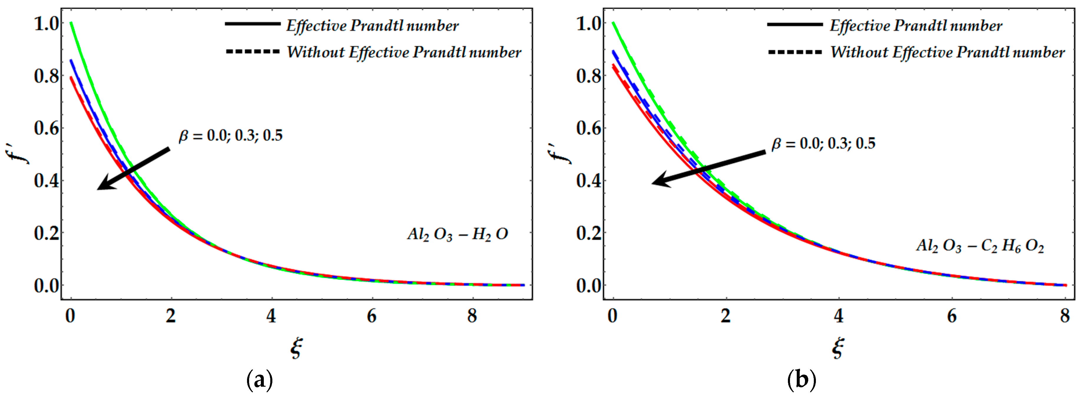
Figure 2.
Velocity curves for different values of (a) For Al2O3-H2O, (b) For Al2O3-C2H6O2.

Figure 3.
Velocity curves for different values of (a) For Al2O3-H2O, (b) For Al2O3-C2H6O2.

Figure 4.
Temperature distribution for different values of . (a) For Al2O3-H2O, (b) For Al2O3-C2H6O2.
Figure 4.
Temperature distribution for different values of . (a) For Al2O3-H2O, (b) For Al2O3-C2H6O2.

Figure 5.
Temperature distribution for different values of . (a) For Al2O3-H2O, (b) For Al2O3-C2H6O2.
Figure 5.
Temperature distribution for different values of . (a) For Al2O3-H2O, (b) For Al2O3-C2H6O2.

Figure 6.
Temperature distribution for different values of (a) For Al2O3-H2O, (b) For Al2O3-C2H6O2.
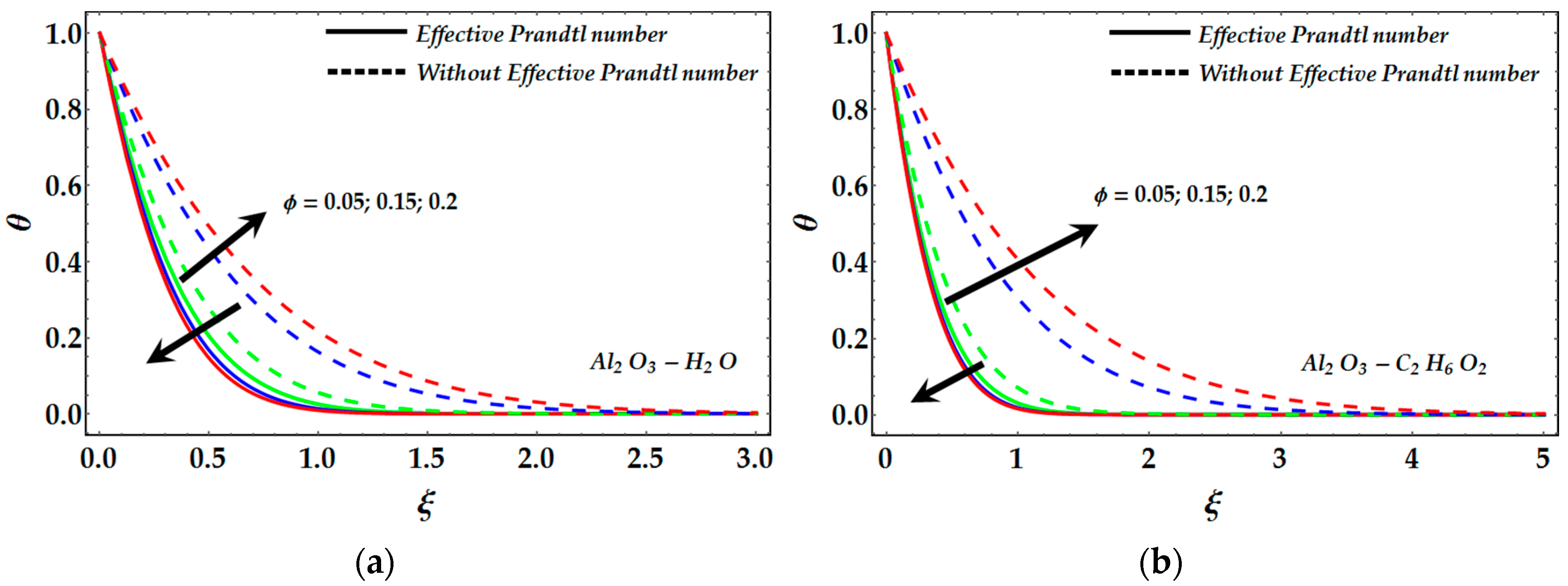
Figure 7.
Entropy generation number for different values of (a) For Al2O3-H2O, (b) For Al2O3-C2H6O2.
Figure 7.
Entropy generation number for different values of (a) For Al2O3-H2O, (b) For Al2O3-C2H6O2.

Figure 8.
Entropy generation number for different values of . (a) For Al2O3-H2O, (b) For Al2O3-C2H6O2.
Figure 8.
Entropy generation number for different values of . (a) For Al2O3-H2O, (b) For Al2O3-C2H6O2.

Figure 9.
Entropy generation number different values of (a) For Al2O3-H2O, (b) For Al2O3-C2H6O2.

Figure 10.
Entropy generation number for different values of Re. (a) For Al2O3-H2O, (b) For Al2O3-C2H6O2.
Figure 10.
Entropy generation number for different values of Re. (a) For Al2O3-H2O, (b) For Al2O3-C2H6O2.

Table 1.
Properties of thermo-physical alumina, water and ethylene glycol.
| (J/kg·K) | (K−1) | (kg/m3) | (W/m·K) | |
|---|---|---|---|---|
| Water (H2O) | 4182 | 20.06 | 998.3 | 0.60 |
| Ethylene glycol (C2H6O2) | 2382 | 65 | 1116.6 | 0.249 |
| Alumina (Al2O3) | 765 | 0.85 | 3970 | 40 |
Table 2.
Numerical comparison of with previously published results.
| λ | Pr | Ali [34] | Grubka and Bobba [35] | Ishak et al. [36] | Present Results |
|---|---|---|---|---|---|
| 0 | 0.72 | 0.8058 | 0.8086 | 0.8086 | 0.80883 |
| 1 | 1.0000 | 1.0000 | 1.0000 | 1.00001 | |
| 3 | 1.9237 | 1.9144 | 1.9237 | 1.92368 | |
| 7 | 3.0723 | 3.07225 | |||
| 10 | 3.7006 | 3.7207 | 3.7207 | 3.72067 | |
| 100 | 12.2940 | 12.2941 | 12.29408 | ||
| 1 | 1 | 1.0873 | 1.08728 | ||
| 2 | 1.1423 | 1.14234 | |||
| 3 | 1.1853 | 1.18528 |
Table 3.
Local Nusselt number and Skin friction coefficient, Numerical values.
| For γAl2O3-H2O | For Al2O3-C2H6O2 | |||||||
|---|---|---|---|---|---|---|---|---|
| With Effective Prandtl Parameter | Without Effective Prandtl Parameter | With Effective Prandtl Parameter | Without Effective Prandtl Parameter | With Effective Prandtl Parameter | Without Effective Prandtl Parameter | With Effective Prandtl Paramet | Without Effective Prandtl Paramet | |
| 1 | 1.29991 | 1.28495 | 1.25372 | 0.78594 | 1.43666 | 1.39986 | 27.6293 | 14.0726 |
| 3 | 1.31432 | 1.30461 | 2.30596 | 1.49072 | 1.45995 | 1.43458 | 50.1784 | 26.4527 |
| 6.96 | 1.32164 | 1.31481 | 3.60726 | 2.36655 | 1.4718 | 1.45394 | 78.076 | 41.9535 |
| 10 | 1.32407 | 1.31821 | 4.35964 | 2.87282 | 1.47573 | 1.46041 | 94.2088 | 50.9162 |
© 2017 by the authors. Licensee MDPI, Basel, Switzerland. This article is an open access article distributed under the terms and conditions of the Creative Commons Attribution (CC BY) license (http://creativecommons.org/licenses/by/4.0/).
Share and Cite
MDPI and ACS Style
Rashidi, M.M.; Abbas, M.A. Effect of Slip Conditions and Entropy Generation Analysis with an Effective Prandtl Number Model on a Nanofluid Flow through a Stretching Sheet. Entropy 2017, 19, 414. https://doi.org/10.3390/e19080414
AMA Style
Rashidi MM, Abbas MA. Effect of Slip Conditions and Entropy Generation Analysis with an Effective Prandtl Number Model on a Nanofluid Flow through a Stretching Sheet. Entropy. 2017; 19(8):414. https://doi.org/10.3390/e19080414
Chicago/Turabian StyleRashidi, Mohammad Mehdi, and Munawwar Ali Abbas. 2017. "Effect of Slip Conditions and Entropy Generation Analysis with an Effective Prandtl Number Model on a Nanofluid Flow through a Stretching Sheet" Entropy 19, no. 8: 414. https://doi.org/10.3390/e19080414
Note that from the first issue of 2016, this journal uses article numbers instead of page numbers. See further details here.