Thermal and Exergetic Analysis of the Goswami Cycle Integrated with Mid-Grade Heat Sources
by
 , ,
, ,
Gokmen Demirkaya
1,† ,
,
Ricardo Vasquez Padilla
2,*,
Armando Fontalvo
3,†,
Maree Lake
2,† and
Yee Yan Lim
2,† 1
Gama Power Systems, Beştepeler Mah. Nergis Sok. No:9 Kat:12, Söğütözü, 06520 Ankara, Turkey
2
School of Environment, Science and Engineering, Southern Cross University, Lismore, NSW 2480, Australia
3
Department of Energy, Universidad de la Costa, Barranquilla 080002, Colombia
*
Author to whom correspondence should be addressed.
†
These authors contributed equally to this work.
Entropy 2017, 19(8), 416; https://doi.org/10.3390/e19080416
Submission received: 26 July 2017
/
Revised: 11 August 2017
/
Accepted: 14 August 2017
/
Published: 17 August 2017
(This article belongs to the Special Issue Work Availability and Exergy Analysis)
Abstract
:This paper presents a theoretical investigation of a combined Power and Cooling Cycle that employs an Ammonia-Water mixture. The cycle combines a Rankine and an absorption refrigeration cycle. The Goswami cycle can be used in a wide range of applications including recovering waste heat as a bottoming cycle or generating power from non-conventional sources like solar radiation or geothermal energy. A thermodynamic study of power and cooling co-generation is presented for heat source temperatures between 100 to 350 °C. A comprehensive analysis of the effect of several operation and configuration parameters, including the number of turbine stages and different superheating configurations, on the power output and the thermal and exergy efficiencies was conducted. Results showed the Goswami cycle can operate at an effective exergy efficiency of 60–80% with thermal efficiencies between 25 to 31%. The investigation also showed that multiple stage turbines had a better performance than single stage turbines when heat source temperatures remain above 200 °C in terms of power, thermal and exergy efficiencies. However, the effect of turbine stages is almost the same when heat source temperatures were below 175 °C. For multiple turbine stages, the use of partial superheating with Single or Double Reheat stream showed a better performance in terms of efficiency. It also showed an increase in exergy destruction when heat source temperature was increased.
1. Introduction
In the last decades, the study of energy systems has been focused on three main directions: the improvement of energy conversion efficiency, the use of clean technologies, and the employment of renewable energy sources like solar radiation, geothermal energy and waste heat from industrial processes [1,2]. To achieve this goal, new thermodynamic cycles have been proposed and some of them have been introduced in the market as competitive commercial alternatives to conventional heat to power cycles such as gas turbines and internal combustion engines. Some of these new thermodynamic cycles employ binary organic fluids mixtures due to their variable and low boiling temperatures during the boiling process, and their good thermal match with the heating fluid which produces an efficient utilization of the heat source [3,4,5]. The new thermodynamic cycles have been proposed for both power production [5,6,7,8,9], and combined power and refrigeration output [4,10]. Among these cycles, the Goswami cycle is one of the widely known combined cycles for simultaneous production of mechanical power and refrigeration supply. This combined cycle is the result of the combination of an ammonia-based organic Rankine cycle and an ammonia-water absorption refrigeration cycle. This cycle can be theoretically used at different scales, be integrated with different heat sources, e.g., solar energy, geothermal energy and waste heat and optimized for power, cooling, thermal or exergy efficiency, depending on the design priorities [4].
Many studies have been conducted on the combined cooling and power system using ammonia–water as working fluid in mid-temperature applications. Some of these promising alternatives have combined the absorption refrigeration cycle with power cycles, mainly based on the Kalina cycle, to produce cooling and mechanical power. Zheng et al. [11] proposed an absorption combined cycle where a rectifier replaced the original flash tank of the Kalina cycle. Sun et al. [12] proposed a modified ammonia-water absorption cycle combined with a Rankine cycle for both power and refrigeration output to recover heat from a 350 °C heat source. The equivalent heat-to-power and exergy efficiencies of this cycle were 18.6% and 42.0% , respectively, and consumed 17.1% less heat than the absorption and the Rankine cycle separated. Later, Yu et al. [13] presented a modified version of Zheng’s cycle with an ammonia refrigeration cycle. According to their results, Yu’s cycle was able to provide cooling and power simultaneously with adjustable ammounts. Zheng reported a 24.2% of thermal efficiency and a 37.3% of exergy efficiency , meanwhile Yu reported an improved thermal efficiency of 37.8%. In both studies, a turbine inlet temperature of 355 °C was adopted. Jin and Zheng [14] took a similar approach of Zheng’s cycle and proposed a modified Kalina cycle coupled with a double effect absorption refrigeration cycle. The new combined cycle produced power and cooling with a co-generation efficiency of 41.2% for a heat source temperature of 465 °C.
In addition, other researchers have studied various combined ammonia-water cycles coupled with mid and low-grade temperature heat sources. Srinivas and Reddy [15] presented a solar combined power and cooling cycle based on an absorption refrigeration system and a Kalina cycle, which was simulated for a solar field outlet temperature of 170 °C. They reported a specific net power output and cooling output of 62.56 kW/kg and 72 kW/kg, respectively. Also, reported results showed a 7–8.85% of heat to power efficiency and up to 7.4% for cooling efficiency. Junye et al.[16] proposed a Kalina cycle with three operation pressures and three new components: a preheater, a water solution cooler and an absorber instead absorption condensers. Simulation results for a turbine inlet temperature of 300 °C showed a first law efficiency of 17.86%. A study from Ayou et al. [17] compared the performance of the Goswami cycle and two new proposed cycles: a Single-stage combined absorption power and a refrigeration cycle with series flow (SSAPRC-S) and a Two-stage combined absorption power and refrigeration cycle with series flow (TSAPRC-S). This study, for an desorber temperature of 220 °C, showed that TSAPRC-S and SSAPRC-S achieved a thermal efficiency of 16.8% and 14.6%, respectively. According to this study, the TSAPRC-S and SSAPRC-S have a better performance than the Goswami cycle at 220 °C of desorber temperature. Rashidi et al. [18] proposed two alternative systems of Kalina cycle coupled with an absorption chiller for low-grade heat sources. The first proposed system included two throttling valves and an evaporator to an ammonia-water based Kalina cycle to generate cooling. In the second system an ammonia-water Kalina cycle provided heat to a Lithium Bromide-water absorption chiller that provides cooling. After performing a parametric analysis, results showed that maximum thermal efficiency was 18.3% for the first system, and 25.9% for the second system. Another study conducted by Cao et al. [19] compared two different alternatives for power and cooling production from low-grade heat sources: a modified Kalina cycle for power and cooling production, and a Kalina cycle coupled with a vapor compression cycle. They reported that the modified Kalina-based power and cooling cycle reached a thermal efficiency of 25.76%, 89.59 kW of power output and 5.58 kW of cooling, meanwhile the Kalina cycle coupled with a vapor compression cycle showed 23.44% of thermal efficiency and 77.81 kW of power output.
With regard to the Goswami cycle, several studies have been proposed to determine the relative advantage of this new technology compared to conventional heat to power applications [20,21,22,23,24,25,26]. Xu et al. [20] carried out a thermodynamic analysis to find the effect of some key parameters like ammonia mass fraction, boiler pressure and temperature on the thermal efficiency and the cooling capacity of the cycle. A second thermodynamic study was performed by Hasan et al. [21] by using a Lorentz cascade arrangement. They found that second law efficiency reached a 65.8% at a heat source temperature of 420 K. Hasan found that, for the studied configuration, an increase in heat source temperature did not increase the second law efficiency. The experimental and theoretical analysis conducted by Martin and Goswami [24] about the performance of the cycle led to a new measure of the effectiveness of cooling production. New configurations of the Goswami cycle have also been proposed and analyzed from the first and second law point of view [25,26]. A comprehensive exergy analysis of two alternative configurations of the cycle was presented by Fontalvo et al. [27]. They determined the effect of some key parameters on the exergy destruction and calculated the contribution of each component of the cycle, showing that the absorber and the boiler had the highest contribution. However, these studies were carried out at heat source temperatures below 420 K. Therefore, the performance of the Goswami cycle has not been studied for higher heat source temperatures, which can be found in solar thermal energy or geothermal sources. The integration of the Goswami cycle with medium heat source temperatures leads to a more complex thermodynamic analysis, since at boiler temperatures above 150 °C the strong solution concentration has a certain range in which an ammonia-water mixture can exist as consequence of the variability of the critical point (temperature and pressure) of the ammonia-water mixture.
This study presents a theoretical thermodynamic analysis of the Goswami cycle for low-Grade and Mid-Grade heat sources. In addition, some modifications to the original Goswami cycle are proposed to improve its thermodynamic integration with Mid-Grade heat sources and overcome some operating restrictions in its components. The aim of this paper is to find the optimum operating conditions and configurations which maximize the performance of the proposed cycle operating at low and medium heat source temperatures, with a boiling temperature in the range of 100 °C to 350 °C. The effect of the different thermodynamic parameters such as: boiling temperature, pressure ratio, reheating, turbine stages on the thermal and exergy efficiencies is analyzed.
2. Thermodynamic Simulation of the Combined Cycle
2.1. Description of the Cycle
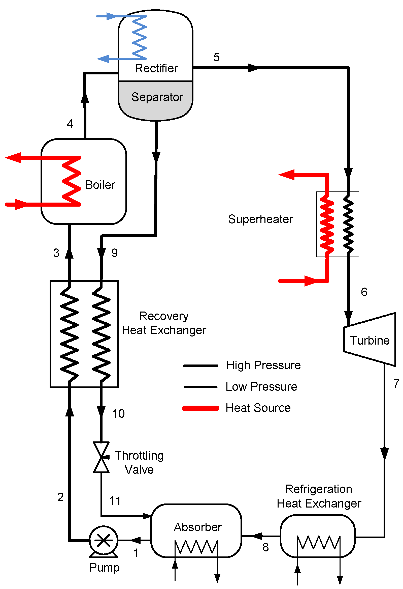
The combined cycle presented in this paper (Figure 1) produces power and refrigeration simultaneously in the same loop and requires less equipment, namely, an absorber, separator, boiler, heat recovery and refrigeration heat exchangers and a turbine. Although the proposed cycle is not restricted to the ammonia-water binary mixtures, it is described here for this working fluid. At state 1, the working fluid leaves the absorber as saturated liquid at the cycle low pressure and then it enters the pump where its pressure is increased to the system high pressure (state 2). After leaving the pump, the fluid is transported to the recovery heat exchanger where it recovers heat from the returning weak ammonia liquid solution and then it enters to the boiler (state 3). In the boiler, the basic solution is partially evaporated to produce a two-phase mixture (state 4): a weak ammonia liquid, with a high concentration of water, and a rich vapor with a very high concentration of ammonia. In the separator, the two phase mixture is separated and the weak liquid (state 9) enters the recovery heat exchanger where it transfers heat to the high concentration stream that comes from the pump. After leaving the recovery heat exchanger, the weak liquid stream (state 10) is throttled to the system low pressure and sprayed into the absorber (state 11). In the rectifier, a cold stream cools the saturated rich ammonia vapor (state 5) to condense out any remaining water. The ammonia stream of state 5 can be superheated (state 6) before it enters to the expander. The expander produces power at the same time it throttles the fluid to the low-pressure of the system (state 7). Under some operating conditions, the temperature of the fluid that leaves the expander in state 7 can be significantly lower than ambient temperature and it can provide cooling output in the refrigeration heat exchanger (state 8). Then, this stream (state 8) rejoins the weak liquid in the absorber where, with heat rejection, the basic solution is regenerated. The status of each point of the cycle is shown in Table 1. In this table, states 7 and 8 are the same because the turbine outlet is very high and the working fluid is not able to provide the cooling effect. Also, the superheater is not active for the results presented in this Table, so states 5 and 6 are the same.
2.2. Thermodynamic Analysis
The cascade cycle analogy [28] provides the suitable efficiency terms to measure the performance of the combined cycle. The effective first law efficiency is given by:
In the above equation, term is the exergy associated with the refrigeration. In order to account for the irreversibilities of heat transfer in the refrigeration heat exchanger, the exergy change of the chilled fluid was considered.
Effective exergy efficiency is given as:
In this Equation, the denominator is the change in exergy of the heat source, which is equivalent to the exergy input.
Exergy analysis is conducted to calculate the destruction of exergy, which is wasted potential for the production of work [29,30]. Hasan and Goswami [22] performed the exergy analysis of the combined power/cooling cycle for heat source temperatures of 47–187 °C, so the same methodology is used here. If the ambient temperature is taken as the reference temperature, then exergy per unit mass of a stream, , is given as:
For a mixture, the exergy is given in terms of exergy of pure components evaluated at component partial pressure and mixture temperature. Szargut [31] suggested that for a binary mixture, exergy could be given in terms of enthalpy, entropy, and composition of mixture as follows:
where x is the mass fraction of one component in the mixture, and and are constants whose values are set arbitrarily such that exergy in the cycle is always positive. It can be shown using material and exergy balances that in calculating the exergy destruction in the cycle for any control volume, the constants and vanish and, therefore, have no effect on the value of exergy destruction in the cycle. As proposed by Hasan and Goswami [22], in this study, and are set as 50 and 250, respectively. The reference state is calculated by using ambient temperature, °C, and the strong solution concentration.
Exergy destruction X is calculated by rearranging the exergy balance equation for a control volume at steady state in the following form [29,30],
where is the work of control volume, m is the mass flow rate, X is exergy destruction within the control volume, Q is the heat transfer with the surroundings or other fluids, and subscripts i and e are used for inlet and exit, respectively. Average temperature is used whenever temperature is not constant. The exergy destruction of each component for the cycle (Figure 1) is as follows: The exergy destruction in the pump, recovery heat exchanger (rhx), boiler heat exchanger (boiler), and separator and rectifier (rect) are given in Equations (7)–(10).
where the subscripts cf refers to the cold fluid used for the rectification cooling needs. The exergy destruction in the superheater heat exchanger, turbine, and refrigeration heat exchanger (refhx) are given Equations (11)–(13).
where the subscripts ref refers to the fluid that will be cooled by the turbine exhaust. The exergy destruction in the absorber and throttling valve (valve) are given Equations (14)–(15).
where the subscripts c to the condensing fluid which is used to regenerate the cycle working fluid. The heat losses from the heat exchangers and other components to the ambient are neglected. The sum of the each component exergy destruction will give the total exergy destruction in the cycle while in steady-state operation.
2.3. Simulation Details
This paper focuses on finding out the maximum performance of the cycle when it utilizes solar thermal energy or geothermal sources, for this reason the boiling temperature is changed between 100 to 350 °C. The cycle parameters for simulation are given in Table 2. Since the pinch point temperature is set at 10 °C, this section covers the heat sources between 110 °C to 360 °C. The design variables for the simulations are boiler pressure, temperature and basic solution concentration while net work output, effective first law and exergy efficiencies are the three main parameters to evaluate the cycle performance.
A computer simulation program is written in Matlab® with the mass and energy balances of the cycle. Also, the thermodynamic properties fo the ammonia-water mixture are calculated using the correlations for thermodynamics properties proposed by Xu and Goswami [32]. The validation of these correlations have been demonstrated by the authors in a previous publication [27], where it was compared with the experimental data obtained by Tillner-Roth and Friend [33]. The following assumptions are used in the thermodynamic analysis:
- The system low pressure is dictated by the strong solution concentration, , and the absorption temperature of 35 °C.
- The boiling conditions are completely specified, i.e., boiling temperature, pressure, and strong solution concentration are provided as inputs.
- Effectiveness value is used for the heat recovery heat exchanger, while pinch point limitation is 10 °C for the boiler, superheater, and refrigeration heat exchangers.
- Superheating is not considered in this simulation, since superheating reduces cooling output.
- Pressure drops are neglected.
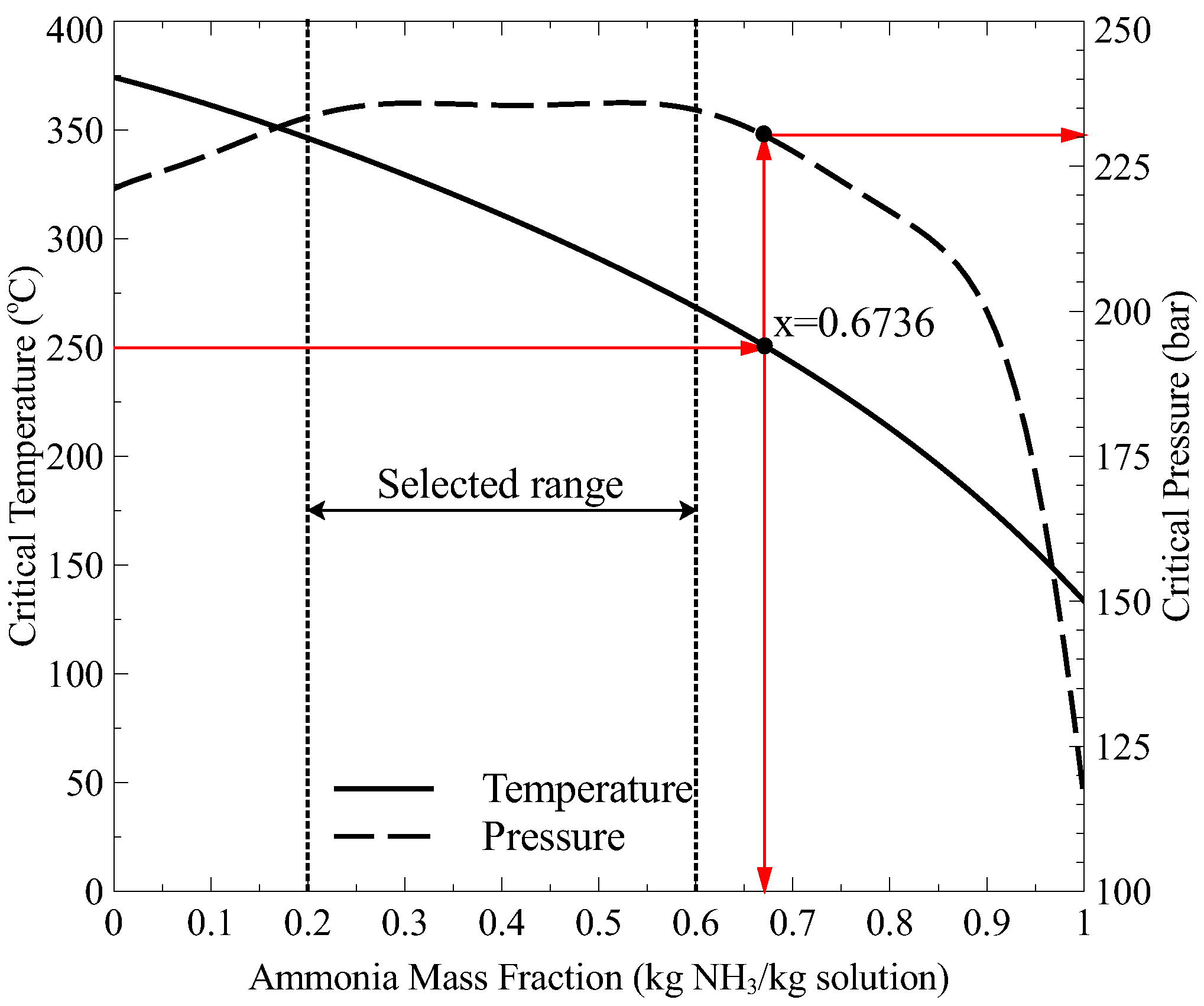
The simulation process is as follows: initially, boiler temperature is specified, and then strong solution concentration is varied for this boiler temperature. This step requires for boiler temperatures above 150 °C, since the strong solution concentration has a certain range in which an ammonia-water mixture can exist. The critical temperature and pressure of the ammonia-water mixture are shown in Figure 2. To give an example, ammonia-water mixture can exist at 250 °C as a saturation mixture if the concentration is less than 0.6736. Therefore, the concentration range for 250 °C was chosen as 0.10 to 0.60 kg NH/kg solution. The same principle applies to other boiler temperatures.
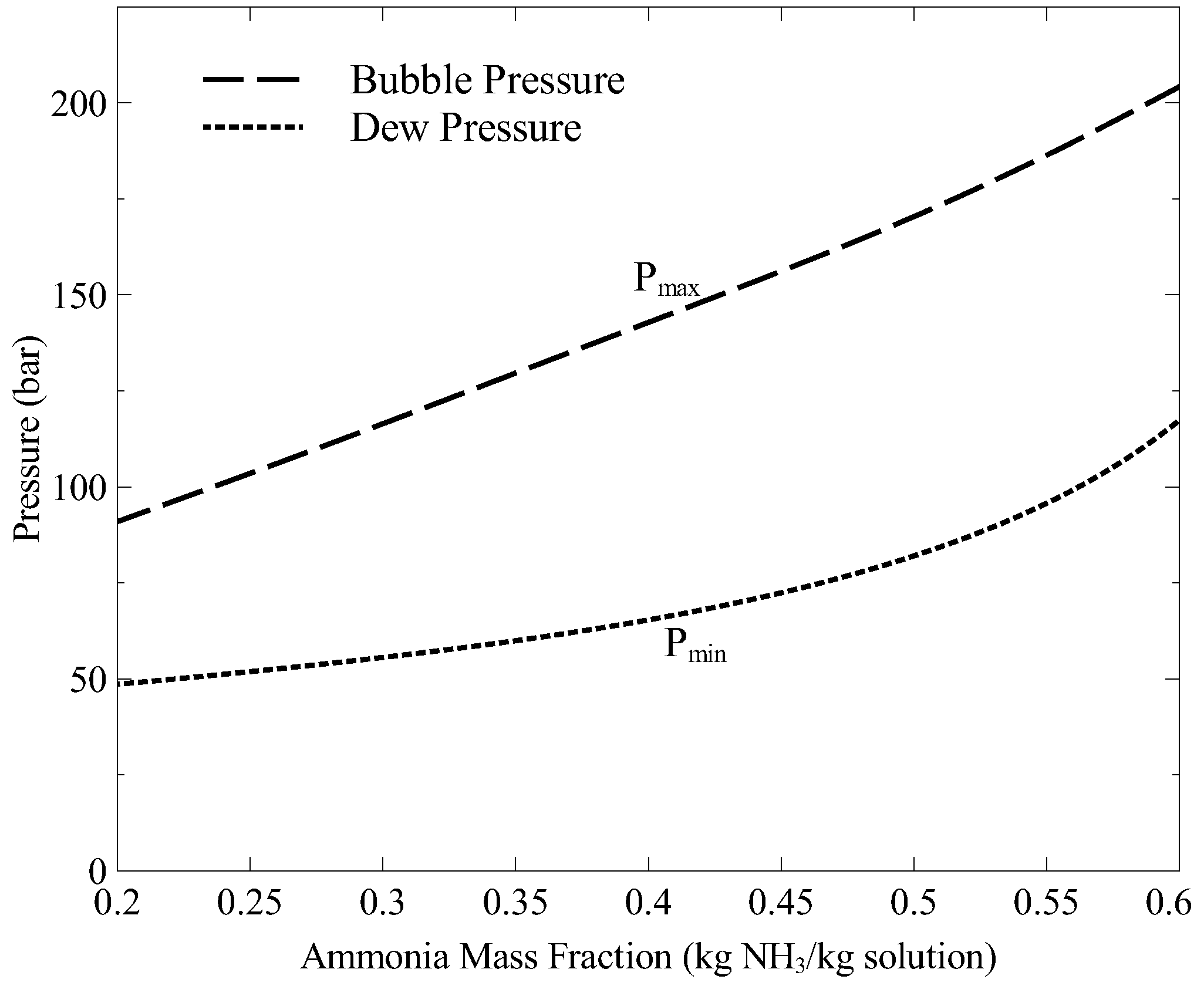
Then dew and bubble pressures for the corresponding temperature and concentration are calculated. In order to have a liquid-vapor saturation mixture at the separator, the system high pressure should be adjusted between the dew and bubble pressures. Figure 3 shows the pressure range at the temperature of 250 °C for different ammonia concentrations. Therefore, the pressure range cannot be fixed and should be updated for every boiler temperature and ammonia concentration. If the pressure is higher than the bubble pressure (142.8 bar at 250 °C and 0.4 kg NH3/kg solution), the solution is in compressed state. If the pressure is lower than the dew pressure (65.4 bar at 250 °C and 0.4 kg NH3/kg solution) all of the solution is vaporized, which will result in no flow through the weak solution line. In the simulations, a minimum ratio of the weak solution return mass flowrate to strong solution mass flowrate is assumed as 10%. Therefore, the cycle performance is evaluated by increasing the boiler pressure, starting from (dew pressure) to (bubble pressure). After defining boiler temperature, pressure, and strong solution concentration, the rectifier exit and superheater temperatures are chosen for the simulation. The cycle performance can be evaluated by using the cycle assumptions given in Table 2 and following inputs: , , , , and .
It is worth mentioning that the turbine exit quality is an important parameter, and it should be taken seriously into account as the presence of liquid droplets in the turbine can cause blade damage and decrease the thermal efficiency of the cycle. Therefore, it is assumed during the simulations that the turbine exit quality cannot be lower than 90%. Simulations show that for the boiler temperature below 150 °C, the turbine exit quality is always higher than 90%, however, in the case of above 150 °C there are some conditions at which the quality drops to lower values. To eliminate low quality exit conditions, expansion stage is increased and reheaters are included in the simulations. If the turbine exit quality is lower than 90%, a two stage turbine is used. The vapor is expanded to a 90% quality through the first turbine, and then reheated and sent to second stage. The turbine exit condition is reviewed again, and the simulation is continued until the turbine exit quality is higher than 90%. Figure 4 shows the effect of reheating and multi-stage expansion. As seen in this figure, both efficiencies are significantly increased with the use of multi-stage turbines. In addition, Figure 4 also presents a comparison between single and multi-stages. For the single stage simulations, if the turbine exit quality is less than 90%, the vapor is expanded through the turbine until the turbine exhaust quality reaches 90%, then the exhaust is throttled to the absorber pressure and sent to the absorber.
3. Alternative Configurations
If the reheating temperature is held constant, the question arises whether the high temperature vapor can be used as waste heat to increase the overall cycle efficiencies. The high temperature vapor can be used as a heat source for a bottoming cycle or a heat recovery system.
Combined Cycle and Vapor Heat Recovery Configurations
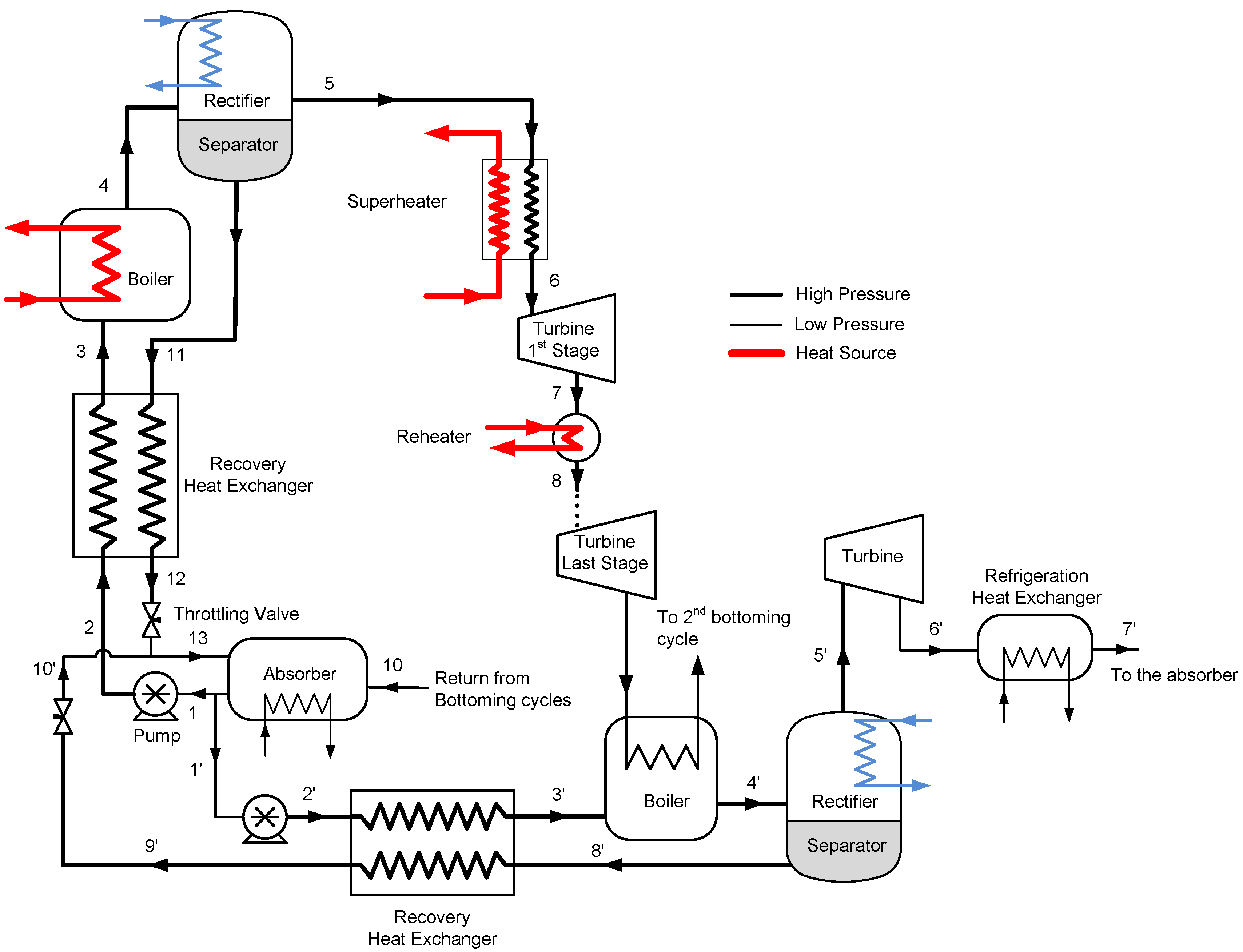
The combined cycle has a top and bottom Goswami cycles. As shown in Figure 5, the turbine exhaust of the top Goswami cycle can be utilized by heating the bottom Goswami cycles working fluid. The simulation of the combined cycle is a complex problem as the optimization of the bottom cycles is also required. The detailed description of the top cycle and the first bottoming cycle are shown in Figure 6. The operating conditions at maximum effective exergy efficiency are used to simulate the top cycle, therefore the mass flow rate and temperature of the vapor are known. The boiler temperature, system high pressure, and strong solution concentration of the bottom cycle will define the temperature of state 8’ as shown in Figure 6, which enters the recovery heat exchanger. The temperature of state 8’ is independent of the strong solution mass flow rate. By performing recovery heat exchanger calculations, the temperature of state 3’ is determined. Then, the boiler heat exchanger calculations are performed and bottom cycle strong solution mass flow rate is found.
The entropy generation in a certain control volume cannot be lower than zero, based on the second law of thermodynamics, and this constraint is applied to all heat exchangers as well as boiler heat exchangers. In the previous analysis, the heat source mass flow rate of the top cycle is calculated based on the pinch point assumption, and then the entropy generation is calculated for the heat exchanger. If the entropy generation term is less than zero, which is an impossible process, the heat source mass flow rate is increased to satisfy the entropy generation constraint. In this case, the top cycle vapor mass flow rate is constant, therefore the bottom cycle mass flow rate is calculated based on the pinch point assumption, and then if the entropy generation term is negative, the pinch point value is increased until the entropy generation is higher than zero. Whenever the pinch point increases, the mass flow rate of the bottom cycle decreases, and the temperature of the top cycle vapor after the heat exchanger might be still high. For this reason, when the top cycle vapor temperature is above 150 °C, two bottom cycles are required to cool down the high temperature vapor of the top cycle to lower than 100 °C.
In order to search the maximum work output from the bottoming cycle, the system high pressure is varied between the bubble and dew point pressures for the corresponding boiler temperature and strong solution concentration.
The vapor heat recovery system is shown in Figure 7. The Goswami cycle system is simpler than the Kalina cycle distillation and condensation subsystems, it has two heat recovery heat exchanger, one separator and a pump as shown in Figure 7. The strong solution is reheated first by the liquid weak solution return from the separator. Then, it is reheated by the high temperature turbine exit vapor, and then it enters the boiler heat exchanger. As described above, entropy generation constraint is also imposed on the vapor heat recovery exchanger.
4. Results and Discussion
4.1. Combined Cycle with Single and Multiple Turbine Stages
4.1.1. Net Work Output
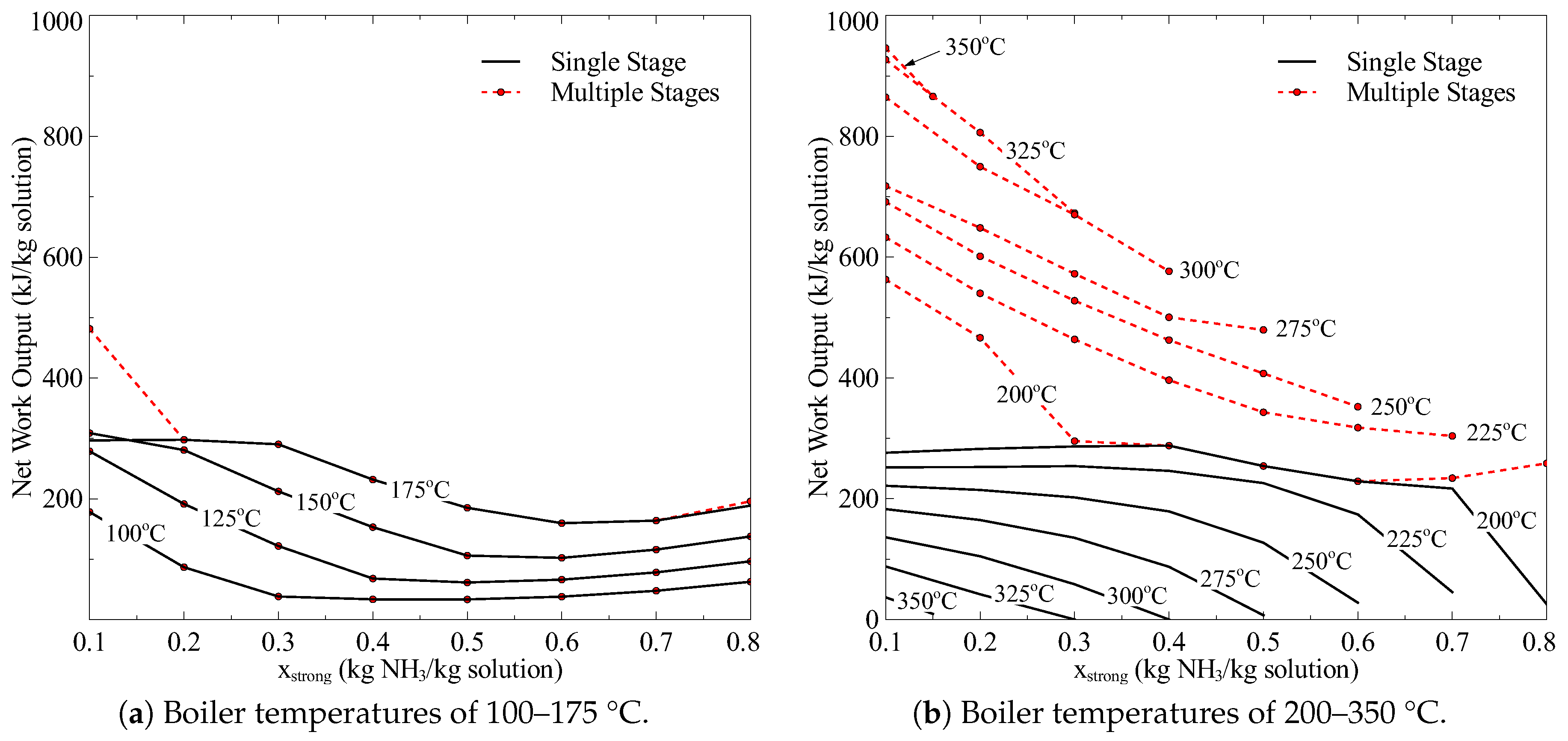
Net work output comparisons of the Goswami cycle with multiple and single turbine stages at boiler temperatures of 100–350 °C are shown in Figure 8. The work output of the Goswami cycle increases with the heat source temperature for the multi-stage expansion case, however it follows a reverse path for the single stage turbine for the heat source temperatures between 200–350 °C as shown in Figure 8b. For the single stage expansion case, the potential of producing more work increases as the pressure ratio is increased; however, the increase in boiler pressure decreases the vapor flow rate for the Goswami cycle, which hinders the potential of producing more work. By adding an additional stage with reheating at a middle pressure between the absorber and the boiler pressures, an additional intermediate pressure is reached by the expansion process and the cycle performs a higher net work output.
The effect of using multi stage turbine is critical above heat sources temperatures of 175 °C, as the system high pressure is varied between the bubble and dew pressures for the corresponding boiler temperature and strong solution concentration, and maximum work output is chosen. Therefore, each point shown in Figure 8 has a different system high pressure, and the only common operating condition is the absorber temperature, which is 35 °C for all cases. The maximum net work occurs at the lowest strong solution for the multi-stage expansion. The enthalpy values of the ammonia-water mixtures increase by decreasing the ammonia concentration, and in addition the system low pressure is at a minimum (~0.25 bar) for the strong solution concentration of 0.1 kg NH3/kg solution. Boiler pressure values for the maximum work output for the boiler temperatures of 100–350 °C are shown in Figure 9. The minimum pressure required at the boiler is 50 bar for 250 °C and higher, however the maximum boiler pressure value for the heat source temperature of 150 °C and lower is approximately 50 bar.
The number of stages used for the multi-stage turbine simulations are given in Table 3. The first additional stage is required at the boiler temperature of 150 °C and the strong solution concentration of 0.1 kg NH3/kg solution. For the low ammonia concentration cases, the turbine exhaust is more prone to wetness because of high water content; this requires an additional reheater and turbine stage when the turbine exhaust is still at higher pressure than the system low pressure. It is seen from Figure 8a that for the boiler temperature of 175 °C and strong solution concentration of 0.1 kg NH3/kg solution, the work output increases significantly for the two stage case compared to single stage case.
4.1.2. Effective First Law Efficiency
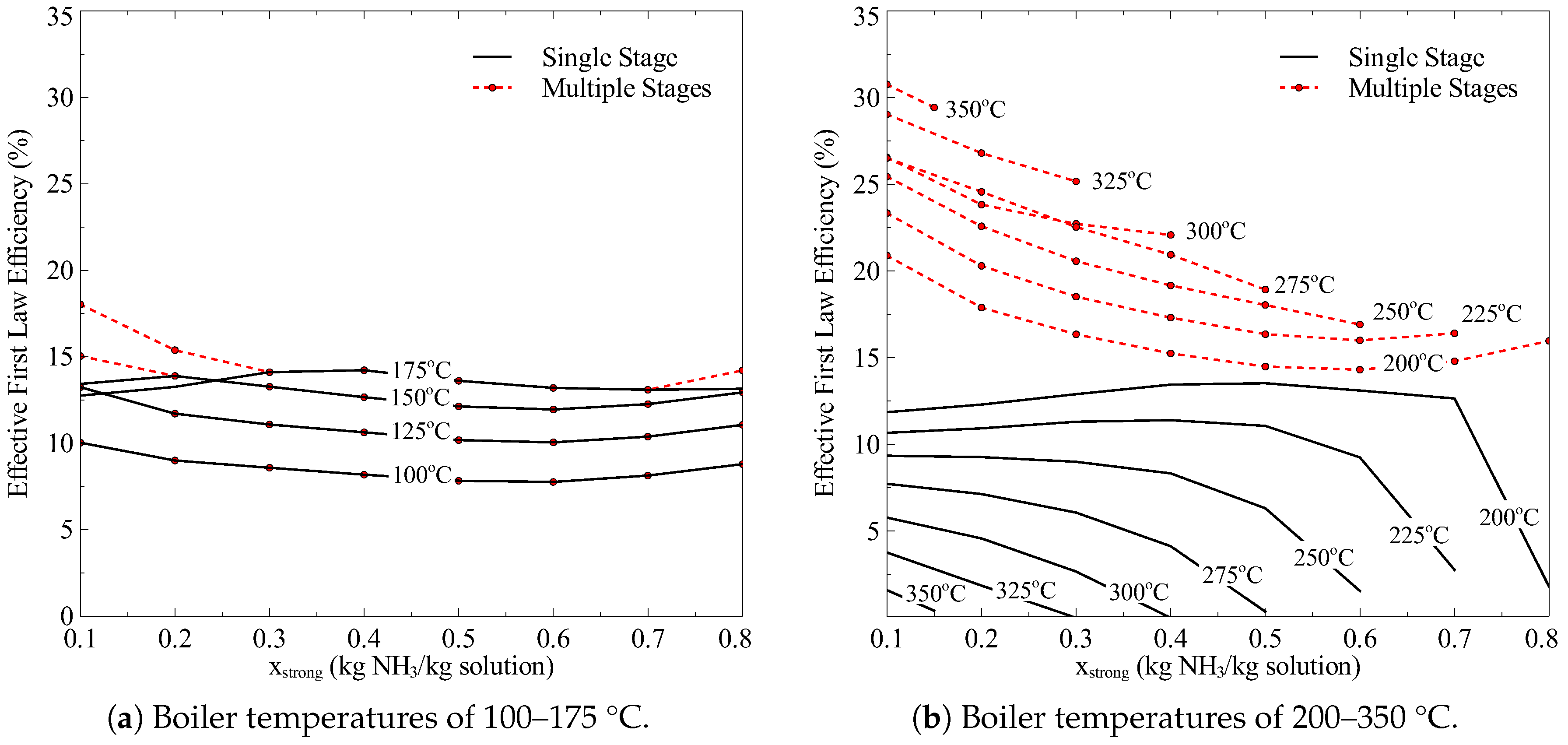
Effective first law efficiency comparisons of the Goswami cycle with multiple and single turbine stages at the boiler temperatures of 100–350 °C are shown in Figure 10. For multiple stage turbines, the maximum effective first law efficiency is between 18–31% for the heat source temperature of 250 °C and 350 °C. If the concentration value of 0.1 is chosen, the maximum effective first law efficiency values are in the 23–31% range. It is also seen in the Figure 10a that single and double stage results are similar for heat source temperatures up to 150 °C. However, the effective first law efficiency values for then multiple stage case is significantly higher than the single stage case for heat source temperatures above 150 °C, as shown in Figure 10b. Above this temperature, the effective first law efficiency is 1.1–19.3 times higher in the multiple stage case compared to the single stage case. It is important to point out that the effective first law efficiency in the single stage case is just 1.6% at 350 °C because the increase in boiler pressure decreases the vapor flow rate for the Goswami cycle, which reduces the work output and the efficiency. Regarding the sensitivity of the effective first law efficiency with ammonia concentration, the results showed no significant changes with the strong solution concentration.
Padilla et al. [25] carried out a power and co-generation analysis of the Goswami cycle with an internal rectification cooling source. In this study, for a boiler temperature between 150–160 ° C, the effective first law efficiency is between 14–15% for a turbine efficiency of 75%, and between 19–20% for a turbine efficiency of 100%. For the multiple stage expansion in this temperature range, the first law efficiency is between 15–17% for a concentration of 0.1 kg NH3/kg solution. These results show that the performance of the multiple stage expansion is very close to the Goswami cycle with an internal rectification cooling source, which is already an improved version of the original cycle as it was stated in [26].
The effective first law efficiency increases as the heat source temperature increases until the boiler temperature of 300 °C. The number of stages required at low concentration is increased to 3 for the boiler temperature of 300 °C; however, the pressure ratio at the last stage is at least 6 times lower than the ratio of 275 °C boiler temperature. As an example, for the boiler temperature of 300 °C and strong solution concentration of 0.1 kg NH3/kg solution, the temperature and pressure of the vapor after the second stage are 94.3 °C and 0.894 bar respectively, and the system low pressure is 0.25 bar. As the fluid pressure is approximately 3.6 times higher than the system low pressure, it could be still utilized to produce work by the third turbine stage. The heat source temperature is assumed to be constant for the boiler and reheaters. Therefore, the exhaust vapor is reheated and expanded to the system low pressure. The temperature of the vapor after the last turbine is 174.9 °C, which is high compared to the previous stage exhaust temperature. If only two stages are used in this case, the effective first law efficiency would be 23.82%, which is lower than the three turbine stage efficiency value of 26.55%. This shows that the cycle efficiency improves with the third stage, however the third stage heat input is not utilized efficiently as the vapor exhaust is still at high temperature, which in this case is 174.9 °C.
4.1.3. Effective Exergy Efficiency
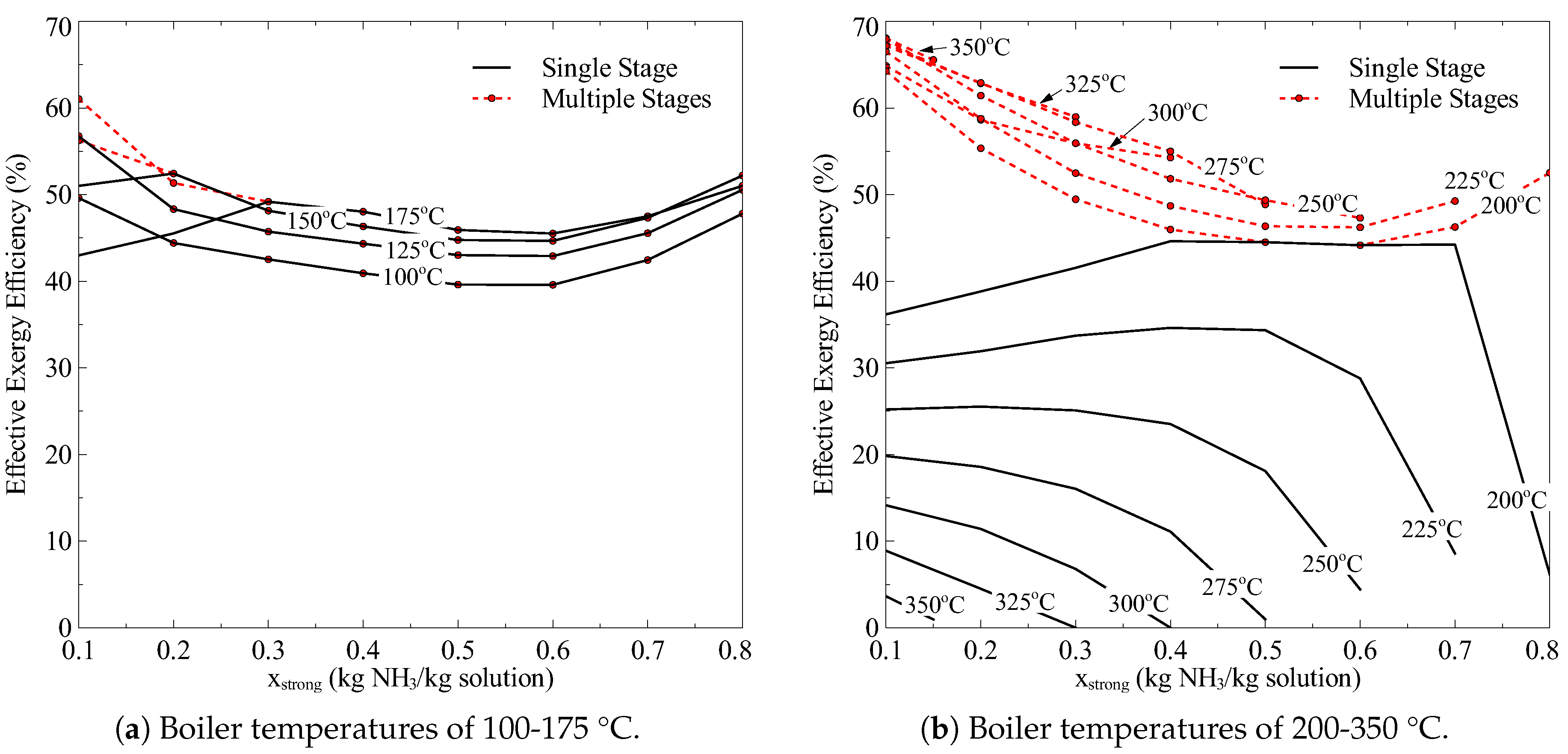
Effective exergy efficiency comparisons of the Goswami cycle with multiple and single turbine stages for boiler temperatures of 100–350 °C are shown in Figure 11. The effective exergy efficiency values are between 40–62% and 45–68% for 100–175 °C and 200–350 °C respectively. As shown in Figure 11b, the effective exergy efficiency values for 300 °C were lower than for 250 °C and 275 °C, due to the reason discussed above. The difference between single and multi-stage expansion for the exergy efficiency is seen clearly in the Figure 11b, with the exergy efficiency decreasing with increasing heat source temperature for the single stage case. These exergy efficiency values are promising when compared to other combined cycles. Sun et al. [12] achieves up to 42.0% of exergy efficiency at a turbine temperature of 350 °C, which is very high compared with the single stage case (), but is also low compared to the multiple stage case ().
It is seen from Figure 11b that the boiler temperatures of 250–275 °C cases have higher exergy efficiency values than 300 °C. As stated above, the cycle requires 3 turbine stages for 300 °C; however, the last stage pressure is not high enough to utilize the reheater effectively.
4.1.4. Exergy Destruction
The exergy destruction in the cycle for different boiler temperatures and basic solution concentrations are shown in Table 4. As seen in this Table, the exergy destruction increases with increasing boiler temperature. When the single and multi-turbine stage cases are compared, it is clear from Table 4 that cycles with the multi-stages have smaller exergy destruction above the boiler temperature of 175 °C. According to Fontalvo et al. [27], when strong solution is fixed at low temperature heat sources, the exergy destruction decreases as the boiler pressure is increased. They point out that the absorber and the boiler have the highest contribution to the exergy destruction, thus a higher pressure and temperature enhances the heat transfer and reduces the entropy generation. When boiler temperatures are above 150 °C, however the cycle operates at low strong solution, which increases the water content across the turbine and increases the turbine outlet temperature as shown in Table 5. A higher turbine outlet temperature reduces the thermal match of the ammonia-water mixture with the cooling fluid in the absorber, which increases the entropy generation. When the multi stage case is considered, the additional stages reduce the turbine outlet temperature, which increases the thermal match of the working and cooling fluid in the absorber and the exergy destruction is reduced.
For the multi-stage case, it is seen from Table 4 that the maximum destruction occurs at the boiler temperature of 300 °C. The sources of exergy destruction in the cycle for a strong solution of 0.1 kg NH3/kg solution (multiple turbine stages) are tabulated in Table 6. The main sources of exergy destruction are heat exchangers, absorber, and turbine stages. For most of the cases, the dominant exergy destruction source is the absorber. These results are in agreement with the exergy destruction distribution reported by Fontalvo et al. [27] and Vidal et al. [34], where the heat transfer equipment and the turbine have the highest contribution to the exergy destruction of the whole cycle. The exergy destruction at the absorber peaks at the boiler temperature of 300 °C. As previously discussed, the last stage turbine temperature is high compared to other cases, which increases the absorber cooling load as well.
4.1.5. Turbine Exit Temperature and Partial Superheating
The turbine exit temperatures of the cycle for all boiler temperatures and strong solution concentrations are shown in Table 5. For multi-turbine stage cases, the turbine exit temperature is maximized for a boiler temperature of 300 °C. The temperature of the vapor after the second turbine for the boiler temperature of 300 °C and strong solution concentration of 0.1 to 0.4 kg NH3/kg solution are 94.3 °C, 107.9 °C, 136.8 °C, and 206.6 °C, respectively. After reheating the vapor to 300 °C temperature, the vapor temperature after the last turbine are 174.9 °C, 203.4 °C, 177.85 °C, and 111.1 °C for the same boiler temperature and strong solution range. As discussed before, the effective exergy efficiency of 300°C boiler case is lower than 275 °C. Therefore, it is obvious that reheating the vapor to 300 °C temperature does not work efficiently.
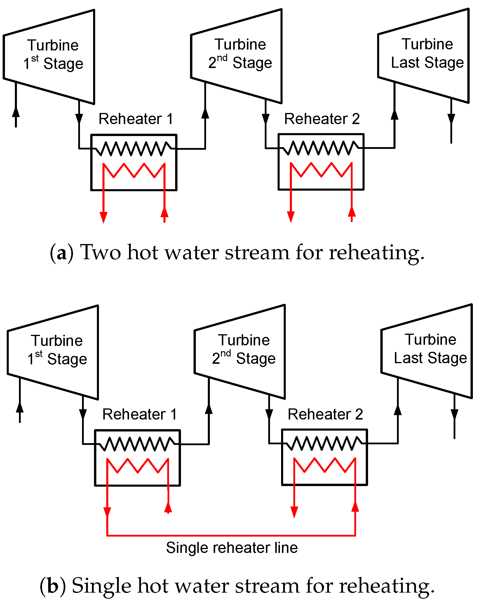
The partial superheating case was conducted to tackle this problem. The vapor is reheated to temperatures less than the boiler temperature and the efficiency values were re-calculated, as there might be a reheating temperature less than 300 °C where efficiency values are higher than the one at 300 °C. To give an example, for the boiler temperature of 300 °C and strong solution of 0.1 kg NH3/kg solution, the vapor temperature after the second turbine was 94.3 °C. The vapor is reheated from 95 °C to 300 °C and the results were compared to find the maximum efficiency. This case is labeled as partial superheating with double reheater stream as two reheater water lines at the same temperature were used. The second option can be using a single reheating stream instead of two for the 3 stage cases. As shown in Figure 12b, the reheating stream after the first reheater is directed to the second reheater. It should be noted that the temperature of the reheating hot water after the first reheater heat exchanger drops, so it is not possible to increase the vapor temperature to boiler temperature at the second reheater, and thus the temperature is always less than the boiler temperature.
To compare the effect of partial superheating, the values at 300 °C are given in Table 7. In general, it can be noticed that the use of Single Reheater stream allowed the development of higher first law and effective exergy efficiency values than Double Reheater stream and reheating to 300 °C, especially at low strong concentrations, where the maximum values were achieved. Although First law efficiencies were very close for Single and Double Reheater stream, with 27.47% for Single Reheater and 27.48% for Double Reheater, the effective exergy efficiency was 67.03% for Single Reheater stream and 66.52% for Double Reheater stream. This trend was maintained even when the strong concentration was increased. It can also be seen that, when it was compared to reheating to 300 °C, the increase in efficiency is between 0.92% and 1.5% for first law efficiency, and between 0.11 and 3.62% for effective exergy efficiency. It should be kept in mind that the partial superheating case with single stream line can be applicable only to the 3 stage cases. The maximum effective first law and exergy efficiencies were updated with the partial superheating cases and given in Table 8.
4.2. Alternative Configurations
With regards to the partial superheating case studied previously, in order to achieve higher efficiency values at high boiler temperatures, the reheating temperature was varied to find the best reheating temperature, which minimizes the exergy losses. In order to examine the possible use of the high temperature vapor, a combined cycle and a vapor heat recovery cases are conducted for the boiler temperature of 300 °C. Firstly, the combined cycle analysis is presented, followed by the vapor heat recovery case, and then the results are presented.
A sensitivity analysis is performed to find the maximum work output from the bottoming cycle. The system high pressure is varied between the bubble and dew point pressures for the corresponding boiler temperature and strong solution concentration. The strong solution concentration is varied between 0.1 and 0.8 kg NH3/kg solution for the bottom cycle simulations.
The combined cycle and vapor heat recovery analysis are conducted for the top cycle boiler temperature of 300 °C. The efficiencies of the analysis are compared with the top cycle alone for the boiler temperatures of 275 °C and 300 °C. The effective first law and exergy efficiencies are shown in Table 9. As it is seen in the table, when the two bottoming cycles are used for the top cycle boiler temperature of 300 °C, the effective first law efficiency increases approximately 1–3.5% compared to the stand alone top cycle. The effective exergy efficiency is also increased approximately 2.5–12.7%. In addition, it is shown in the Table 9 that the efficiency terms of 300 °C case are increased compared to the boiler temperature of 275 °C case by utilizing the turbine exhaust vapor. The vapor heat recovery system improves the efficiencies significantly for the concentration values of 0.1 and 0.2. Due to the entropy generation constraint, this system cannot be used for the strong solution concentration of 0.4 kg NH3/kg solution. It is noteworthy that the use of bottoming cycles and vapor heat recovery system requires additional equipment, which will incur additional cost; however, the cost can be reduced if some components like the absorber can be shared with cycles. If the same absorber is used for top and bottom cycles, the cost of the absorber per unit size can be reduced. The combined system can provide additional work, which would increase the overall capacity; on the other hand, the vapor heat recovery system can increase the cycle efficiencies significantly with an additional heat exchanger.
4.3. Comparison with Other Cycles
Junye et al. [16] proposed a Kalina cycle with three operation pressures and three new components: a preheater, a water solution cooler and an absorber, instead of absorption condensers. Simulations results were reported for a turbine inlet temperature of 300 °C and compared with two steam Rankine cycles (SRC). According to the simulation results, the multi-stage turbine clearly improves the performance of the Goswami cycle when it is compared to Junye’s cycle because it performs between 22.1–27.5% of effective first law efficiency at the same inlet turbine temperature while the Junye’s cycle achieves up to 17.86% and the SRCs develops 23.24%. A study from Ayou et al., [17] compares the performance of the Goswami cycle and two new proposed cycles: a Single-stage combined absorption power and refrigeration cycle with series flow (SSAPRC-S) and a Two-stage combined absorption power and refrigeration cycle with series flow (TSAPRC-S). This study, for an desorber temperature of 220 °C, shows that TSAPRC-S and SSAPRC-S reach a thermal efficiency of 16.8% and 14.6%, respectively. According to this study, the TSAPRC-S and SSAPRC-S have a better performance than the Goswami cycle at 220 °C of desorber temperature. However, in the multi-stage expansion case, the Goswami cycle is able to obtain a effective first law efficiency of 23.34% for a boiler temperature of 225 °C, and 21% for 200 °C. These results reveal that the multiple stage expansion improves the efficiency of the Goswami and makes it more efficient than the TSAPRC-S and SSAPRC-S cycles.
Dincer and Al-Muslim [35] conducted a thermodynamic analysis of the steam power plants with reheat. The temperature and pressure values were in the range between 400 and 590 °C, and 100 and 150 bar respectively. The first law and exergy efficiencies for the corresponding boiler temperature range were approximately 38–43% and 53–58%. Kalina [3] investigated the Kalina cycle performance for a boiler temperature of 532 °C and found that the bottoming cycle produces 2.7 MWe with first law and exergy efficiencies of 32.9% and 70.0% respectively. Nag and Gupta [36] examined the exergy analysis of the Kalina cycle. They varied the temperature of ammonia-water mixture at the condenser, and found that the cycle efficiency varies between 30–36% for a boiler temperature of 500 °C. The second law efficiency for the same operating conditions is in the range of 51–60%. In an another Kalina cycle study, Olsson et al. [37] found the first law and exergy efficiencies of 23% and 69.7%, respectively for the turbine inlet pressure of 110 bar and a temperature of 494 °C.
Table 10 shows a summary of some power and cooling applications that can be found in literature. Thermal and exergy efficiencies can also be consulted in this table, as well as their Carnot efficiency, based on the condenser and boiler temperatures reported by the authors in the respective references. Compared to other ammonia-water based power and cooling cycles, the Goswami cycle is able to develop more net power output and achieves higher values of effective first law and exergy efficiency. In addition when boiler temperature is above 300 °C, the use of bottoming cycles and vapor heat recovery system exhibit higher first law efficiencies (28.49–30.84%) at a strong solution concentration of 0.1 kg NH3/kg solution, showing a higher performance in terms of first law efficiency than the combined Kalina and absorption refrigeration cycles presented in Table 10. However, as it was stated above, these configurations require additional equipment that will incur additional cost.
In summary, the Goswami cycle can operate at an effective exergy efficiency of 60–68% with the boiler temperature range of 200–350 °C. The first law efficiency of 25–31% can be achievable with the boiler temperatures of 250–350 °C. In addition, this cycle can utilize low temperature sources such as 60–100 °C to produce work and cooling simultaneously as proven by the authors in their previous studies [25,26].
5. Conclusions
A theoretical analysis of a combined power and cooling cycle was conducted to find out the maximum performance of the cycle when it utilizes mid-grade thermal sources. The effect of cycle parameters, cycle configurations and components on the performance of the system in terms of net power output, first law and effective exergy efficiencies, and exergy destruction was determined. The following conclusions were obtained:
- Multiple turbine stages in Goswami cycle developed higher power output, first law and effective exergy efficiencies than single turbine stage when boiler temperatures are between 200 and 300 °C. However, the performance of single and multiple stages is almost the same for boiler temperatures below 175 °C and a strong concentration solution concentration greater than 0.1 kg NH3/kg solution.
- When boiler temperatures in the Goswami cycle are above 175 °C, higher pressures can be developed but the operation is restricted to low strong solution concentrations, which leads to low turbine outlet quality below 90%. In this case, the use of multiple stage turbines increases the performance of the cycle and avoids the quality restriction at the turbine outlet.
- Since the exergy destruction increases with the boiler temperature, the use of multiple turbine stages allows a reduction in the increase in exergy destruction due to the turbine, when compared to the single turbine stage. It was also found that including an additional stage reduced the turbine contribution to exergy destruction at two specific boiler temperatures: 150 °C and 300 °C.
- For multiple turbine stages, the use of partial superheating with Single or Double Reheat stream showed a better performance in terms of efficiency, with an increase in percentage points between 0.92–1.5%, and 0.11–3.62% for first law efficiency and effective exergy efficiency, respectively.
- When the boiler temperature is above 275 °C, the use of two additional bottom cycles or a vapor heat recovery system improves the cycle performance compared to the stand alone top cycle. The increase in efficiency terms is between 1 and 3.5% for first law efficiency, and between 2.5 and 12.7% for effective exergy efficiency.
Acknowledgments
The research leading to this paper was funded by the State of Florida through the Florida Energy Systems Consortium (FESC) funds.
Author Contributions
Gokmen Demirkaya and Ricardo Vasquez Padilla conceived and made the simulations of the thermodynamic model. Armando Fontalvo helped with the literature review. Gokmen Demirkaya, Ricardo Vasquez Padilla and Armando Fontalvo wrote the paper. Maree Lake and Yee Yan Lim edited the paper. All authors worked equally in the analysis and discussion of the results. All authors have read and approved the final manuscript.
Conflicts of Interest
The authors declare no conflict of interest.
Abbreviations
The following abbreviations and symbols are used in this manuscript:
| Q | Specific heat transfer () |
| T | Temperature (°C or K) |
| E | Specific exergy () |
| h | Specific enthalpy () |
| s | Specific entropy () |
| m | Mass flow ratio () |
| W | Specific work () |
| X | Specific exergy destruction () |
| x | Ammonia concentration () |
| Subscripts | |
| c | Cooling |
| h | Heat |
| Chilled fluid | |
| Exergy | |
| Effective value | |
| I | First law |
| Exergy | |
| Inlet | |
| Heat source | |
| Net | |
| Outlet | |
| o | Reference |
| Refrigeration | |
| Greek symbols | |
| Effectiveness, exergy per unit mass of a stream () | |
| Constant to calculate exergy of a binary mixture | |
| Constant to calculate exergy of a binary mixture | |
| Efficiency | |
References
- Cruz Virosa, I.; Filgueiras Sainz de Rozas, M.L.; Sorinas Gonzáles, L.; Cabello Eras, J.J.; Fernández Pérez, L. Gestión comparada del riesgo en el control de la contaminación atmosférica de Generadores de Vapor. Ingeniería Energética 2016, 37, 195–206. (In Spanish) [Google Scholar]
- Eras, J.J.C.; Gutiérrez, A.S.; Lorenzo, D.G.; Martínez, J.B.C.; Hens, L.; Vandecasteele, C. Bridging universities and industry through cleaner production activities. Experiences from the Cleaner Production Center at the University of Cienfuegos, Cuba. J. Clean. Prod. 2015, 108, 873–882. [Google Scholar] [CrossRef]
- Kalina, A.I. Combined Cycle System with Novel Bottoming Cycle. J. Eng. Gas Turbines Power 1984, 106, 737–742. [Google Scholar] [CrossRef]
- Goswami, D.Y. Solar Thermal Power: Status of Technologies and Opportunities for Research. Heat Mass Transf. Conf 1995, 95, 57–60. [Google Scholar]
- Ibrahim, O.M.; Klein, S.A. Absorption Power Cycles. Energy 1996, 21, 21–27. [Google Scholar] [CrossRef]
- Maloney, J.D.; Robertson, R.C. Thermodynamic Study of Ammonia-Water Heat Power Cycles; Technical Report CF-53-8-43; National Laboratory: Oak Ridge, TN, USA, 1953. [Google Scholar]
- Kalina, A.I. Combined cycle and waste heat recovery power systems based on a novel thermodynamic energy cycle utilizing low-temperature heat for power generation. In Proceedings of the 1983 Joint Power Generation Conference: GT Papers, Indianapolis, IN, USA, 25–29 September 1983. [Google Scholar] [CrossRef]
- Marston, C.H. Parametric analysis of the Kalina cycle. J. Eng. Gas Turbines Power 1990, 112, 107–116. [Google Scholar] [CrossRef]
- Park, Y.M.; Sonntag, R.E. A Preliminary Study of the Kalina Power Cycle in Connection with a Combined Cycle System. Int. J. Energy. Res. 1990, 14, 153–162. [Google Scholar] [CrossRef]
- Goswami, D.Y. Solar thermal power technology: Present status and ideas. Energy Sources 1998, 20, 137–145. [Google Scholar] [CrossRef]
- Zheng, D.; Chen, B.; Qi, Y.; Jin, H. Thermodynamic analysis of a novel absorption power/cooling combined-cycle. Appl. Energy 2006, 83, 311–323. [Google Scholar] [CrossRef]
- Sun, L.; Han, W.; Jing, X.; Zheng, D.; Jin, H. A power and cooling cogeneration system using mid/low-temperature heat source. Appl. Energy 2013, 112, 886–897. [Google Scholar] [CrossRef]
- Yu, Z.; Han, J.; Liu, H.; Zhao, H. Theoretical study on a novel ammonia–water cogeneration system with adjustable cooling to power ratios. Appl. Energy 2014, 122, 53–61. [Google Scholar] [CrossRef]
- Jing, X.; Zheng, D. Effect of cycle coupling-configuration on energy cascade utilization for a new power and cooling cogeneration cycle. Energy Convers. Manag. 2014, 78, 58–64. [Google Scholar] [CrossRef]
- Srinivas, T.; Reddy, B.V. Thermal optimization of a solar thermal cooling cogeneration plant at low temperature heat recovery. J. Energy Resour. Technol. 2014, 136, 021204. [Google Scholar] [CrossRef]
- Hua, J.; Chen, Y.; Wu, J. Thermal performance of a modified ammonia–water power cycle for reclaiming mid/low-grade waste heat. Energy Convers. Manag. 2014, 85, 453–459. [Google Scholar] [CrossRef]
- Ayou, D.S.; Bruno, J.C.; Coronas, A. Combined absorption power and refrigeration cycles using low- and mid-grade heat sources. Sci. Technol. Built Environ. 2015, 21, 934–943. [Google Scholar] [CrossRef]
- Rashidi, J.; Ifaei, P.; Esfahani, I.J.; Ataei, A.; Yoo, C.K. Thermodynamic and economic studies of two new high efficient power-cooling cogeneration systems based on Kalina and absorption refrigeration cycles. Energy Convers. Manag. 2016, 127, 170–186. [Google Scholar] [CrossRef]
- Cao, L.; Wang, J.; Wang, H.; Zhao, P.; Dai, Y. Thermodynamic analysis of a Kalina-based combined cooling and power cycle driven by low-grade heat source. Appl. Therm. Eng. 2017, 111, 8–19. [Google Scholar] [CrossRef]
- Xu, F.; Goswami, D.Y.; Bhagwat, S.S. A combined power/cooling cycle. Energy 2000, 25, 233–246. [Google Scholar] [CrossRef]
- Hasan, A.A.; Goswami, D.Y.; Vijayaraghavan, S. First and second law analysis of a new power and refrigeration thermodynamic cycle using a solar heat source. Sol. Energy 2002, 73, 385–393. [Google Scholar] [CrossRef]
- Hasan, A.A.; Goswami, D.Y. Exergy Analysis of a Combined Power and Refrigeration Thermodynamic Cycle Driven by a Solar Heat Source. J. Sol. Energy Eng. 2003, 125, 55–60. [Google Scholar] [CrossRef]
- Martin, C.; Goswami, D.Y. Analysis of Experimental Power and Cooling Production in a Combined Power and Cooling Cycle. In Proceedings of the 17th International Conference on Efficiency, Costs, Optimization, Simulation and Environmental Impact of Energy on Process Systems, Guanajuato City, Mexico, 2004; pp. 1235–1244. [Google Scholar]
- Martin, C.; Goswami, D.Y. Effectiveness of cooling production with a combined power and cooling thermodynamic cycle. Appl. Therm. Eng. 2006, 26, 576–582. [Google Scholar] [CrossRef]
- Padilla, R.V.; Demirkaya, G.; Goswami, D.Y.; Stefanakos, E.; Rahman, M.M. Analysis of power and cooling cogeneration using ammonia-water mixture. Energy 2010, 35, 4649–4657. [Google Scholar] [CrossRef]
- Demirkaya, G.; Padilla, R.V.; Goswami, D.Y.; Stefanakos, E.; Rahman, M.M. Analysis of a combined power and cooling cycle for low-grade heat sources. Int. J. Energy Res. 2011, 35, 1145–1157. [Google Scholar] [CrossRef]
- Fontalvo, A.; Pinzon, H.; Duarte, J.; Bula, A.; Quiroga, A.G.; Padilla, R.V. Exergy analysis of a combined power and cooling cycle. Appl. Therm. Eng. 2013, 60, 164–171. [Google Scholar] [CrossRef]
- Vijayaraghavan, S.; Goswami, D.Y. On Evaluating Efficiency of a Combined Power and Cooling Cycle. J. Energy Resour. Technol. 2003, 125, 221–227. [Google Scholar] [CrossRef]
- Cengel, Y.A.; Boles, M.A. Thermodynamics: An Engineering Approach; McGraw-Hill: New York, NY, USA, 2002. [Google Scholar]
- Moran, M.J.; Shapiro, H.N.; Boettner, D.D.; Bailey, M. Fundamentals of Engineering Thermodynamics; John Wiley & Sons Inc.: Hoboken, NJ, USA, 2010. [Google Scholar]
- Szargut, J.; Morris, D.R.; Steward, F.R. Energy Analysis of Thermal, Chemical, and Metallurgical Processes; Hemisphere Publishing: Panama City, Panama, 1988. [Google Scholar]
- Xu, F.; Goswami, D.Y. Thermodynamic properties of ammonia–water mixtures for power-cycle applications. Energy 1999, 24, 525–536. [Google Scholar] [CrossRef]
- Tillner-Roth, R.; Friend, D. A Helmholtz free energy formulation of the thermodynamic properties of the mixture water + ammonia. J. Phys. Chem. Ref. Data 1998, 27, 63. [Google Scholar] [CrossRef]
- Vidal, A.; Best, R.; Rivero, R.; Cervantes, J. Analysis of a combined power and refrigeration cycle by the exergy method. Energy 2006, 31, 3401–3414. [Google Scholar] [CrossRef]
- Dincer, I.; Al-Muslim, H. Thermodynamic analysis of reheat cycle steam power plants. Int. J. Energy Res. 2001, 25, 727–739. [Google Scholar] [CrossRef]
- Nag, P.; Gupta, A. Exergy analysis of the Kalina cycle. Appl. Ther. Eng. 1998, 18, 427–439. [Google Scholar] [CrossRef]
- Olsson, E.; Desideri, U.; Stecco, S.; Svedberg, G. An integrated gas turbine-Kalina cycle for cogeneration. In Proceeding of the 36th ASME International Gas Turbine and Aeroengine Congress and Exposition, Orlando, FL, USA, 3–6 June 1991; pp. 1–6. [Google Scholar]
- Erickson, D.C.; Anand, G.; Kyung, I. Heat-activated dual-function absorption cycle. ASHRAE Trans. 2004, 110, 515–524. [Google Scholar]
- Wang, J.; Dai, Y.; Zhang, T.; Ma, S. Parametric analysis for a new combined power and ejector–absorption refrigeration cycle. Energy 2009, 34, 1587–1593. [Google Scholar] [CrossRef]
- Wang, J.; Dai, Y.; Gao, L. Parametric analysis and optimization for a combined power and refrigeration cycle. Appl. Energy 2008, 85, 1071–1085. [Google Scholar] [CrossRef]
- Takeshita, K.; Amano, Y.; Hashizume, T. Experimental study of advanced cogeneration system with ammonia–water mixture cycles at bottoming. Energy 2005, 30, 247–260. [Google Scholar] [CrossRef]
- Jawahar, C.P.; Saravanan, R.; Bruno, J.C.; Coronas, A. Simulation studies on gax based Kalina cycle for both power and cooling applications. Appl. Therm. Eng. 2013, 50, 1522–1529. [Google Scholar] [CrossRef]
- Hua, J.; Chen, Y.; Wang, Y.; Roskilly, A.P. Thermodynamic analysis of ammonia–water power/chilling cogeneration cycle with low-grade waste heat. Appl. Therm. Eng. 2014, 64, 483–490. [Google Scholar] [CrossRef]
- Liu, M.; Zhang, N. Proposal and analysis of a novel ammonia-water cycle for power and refrigeration cogeneration. Energy 2007, 32, 961–970. [Google Scholar] [CrossRef]
- Zhang, N.; Lior, N. Development of a novel combined absorption cycle for power generation and refrigeration. J. Energy Resour. Technol. 2007, 129, 254–265. [Google Scholar] [CrossRef]
Figure 1.
Schematic description of the Goswami cycle with internal cooling.

Figure 2.
Critical temperature and pressure of the ammonia-water mixture.

Figure 3.
Bubble and dew pressure of the ammonia-water mixture at 250 °C.

Figure 4.
Effective first law and exergy efficiencies for (a) single and (b) multi-stage turbines at a boiler temperature of 250 °C.
Figure 4.
Effective first law and exergy efficiencies for (a) single and (b) multi-stage turbines at a boiler temperature of 250 °C.
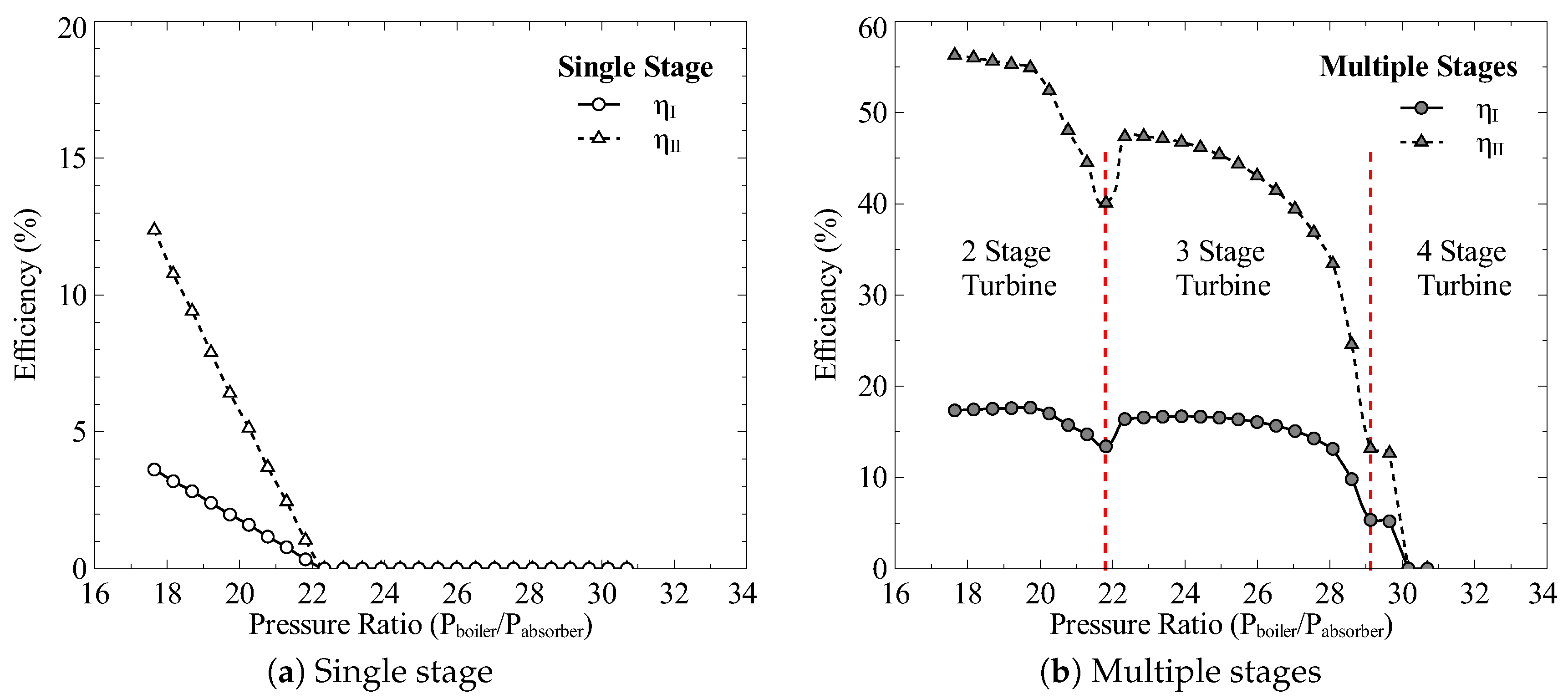
Figure 5.
Schematic description of the combined cycle, top and bottom Goswami cycles.
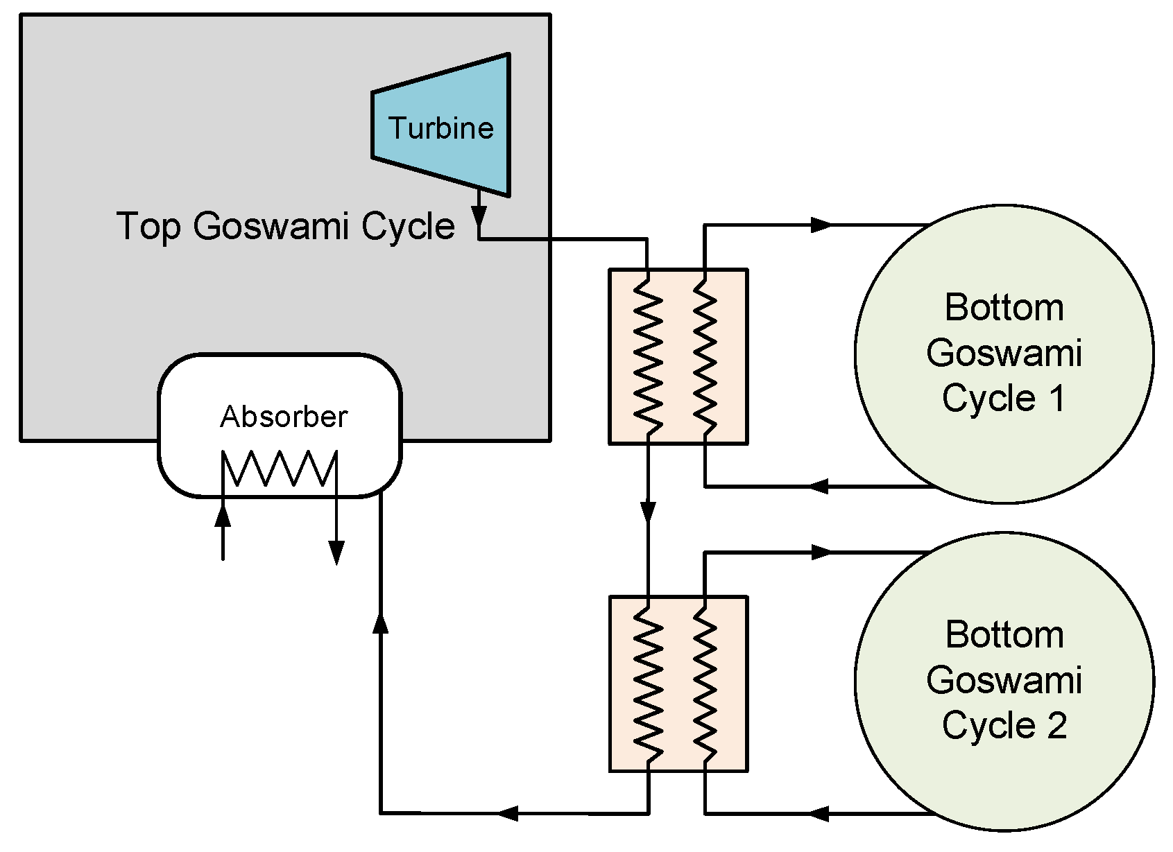
Figure 6.
Detailed description of the combined cycle, top and the first bottoming Goswami cycles.

Figure 7.
Schematic description of the vapor heat recovery system.
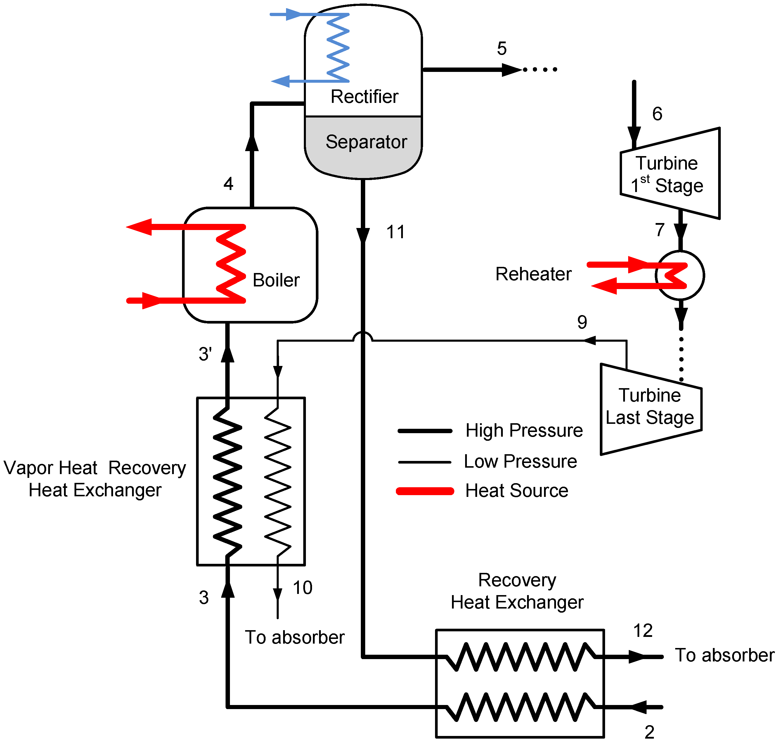
Figure 8.
Net work output comparison of the Goswami cycle at different boiler temperatures for single and multiple turbine stages.
Figure 8.
Net work output comparison of the Goswami cycle at different boiler temperatures for single and multiple turbine stages.

Figure 9.
Boiler pressure values at boiler temperatures of 100–350 °C.
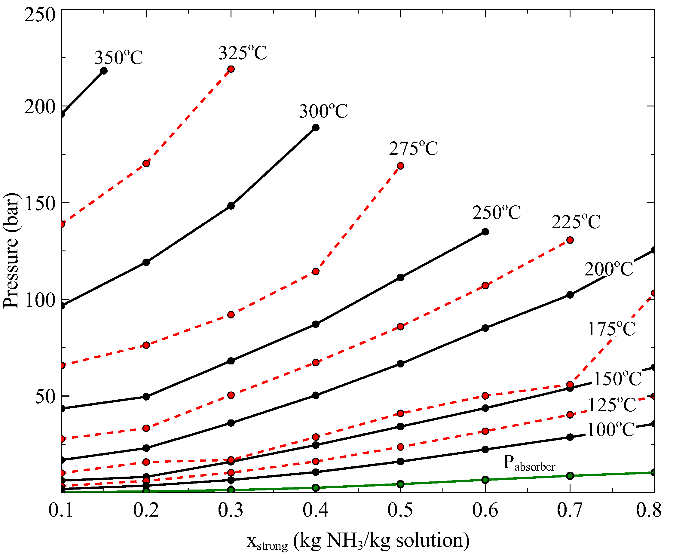
Figure 10.
Effective first law efficiency comparison of the Goswami cycle at different boiler temperatures for single and multiple turbine stages.
Figure 10.
Effective first law efficiency comparison of the Goswami cycle at different boiler temperatures for single and multiple turbine stages.

Figure 11.
Effective exergy efficiency comparison of the Goswami cycle at different boiler temperatures for single and multiple turbine stages.
Figure 11.
Effective exergy efficiency comparison of the Goswami cycle at different boiler temperatures for single and multiple turbine stages.

Figure 12.
Partial superheating cases.


Table 1.
Operation parameters and enthalpy values of the Goswami cycle. Boiler Temperature of 250 °C.
Table 1.
Operation parameters and enthalpy values of the Goswami cycle. Boiler Temperature of 250 °C.
| States | Temperature (K) | Pressure (bar) | Enthalpy (kJ/kg) | Mass Flow (kg/s) | Ammonia Mass Fraction |
|---|---|---|---|---|---|
| 1 | 308.2 | 6.65 | 1.0 | 0.6 | |
| 2 | 311.0 | 117.38 | 1.0 | 0.6 | |
| 3 | 418.9 | 117.38 | 528.07 | 1.0 | 0.6 |
| 4 | 523.2 | 117.38 | 2034.1 | 1.0 | 0.6 |
| 5 | 479.4 | 117.38 | 1690.8 | 0.28 | 0.8 |
| 6 | 479.4 | 117.38 | 1690.8 | 0.28 | 0.8 |
| 7 | 363.5 | 6.65 | 1319.1 | 0.28 | 0.8 |
| 8 | 363.5 | 6.65 | 1319.1 | 0.28 | 0.8 |
| 9 | 479.4 | 117.38 | 865.2 | 0.72 | 0.52 |
| 10 | 340.3 | 117.38 | 96.2 | 0.72 | 0.52 |
| 11 | 325.9 | 6.65 | 96.2 | 0.72 | 0.52 |
Table 2.
Cycle parameters assumed for the theoretical study.
| Parameter | Value | Units |
|---|---|---|
| Pinch Point | 10 | °C |
| Reference Temperature | 25 | °C |
| Reference Pressure | 1 | bar |
| Second law efficiency of refrigeration [28] | 30% | |
| Recovery heat exchanger effectiveness | 85% | |
| Isentropic turbine efficiency | 85% | |
| Minimum turbine exit vapor quality | 90% | |
| Isentropic pump efficiency | 85% |
Table 3.
The number of stages used for multi-stage turbine case.
| x (kg NH/kg Solution) | ||||||||
|---|---|---|---|---|---|---|---|---|
| T (°C) | 0.1 | 0.2 | 0.3 | 0.4 | 0.5 | 0.6 | 0.7 | 0.8 |
| 100 | 1 | 1 | 1 | 1 | 1 | 1 | 1 | 1 |
| 125 | 1 | 1 | 1 | 1 | 1 | 1 | 1 | 1 |
| 150 | 2 | 1 | 1 | 1 | 1 | 1 | 1 | 1 |
| 175 | 2 | 2 | 1 | 1 | 1 | 1 | 1 | 1 |
| 200 | 2 | 2 | 2 | 2 | 1 | 1 | 1 | 1 |
| 225 | 2 | 2 | 2 | 2 | 2 | 2 | 2 | |
| 250 | 2 | 2 | 2 | 2 | 2 | 2 | ||
| 275 | 2 | 2 | 2 | 2 | 3 | |||
| 300 | 3 | 3 | 3 | 3 | ||||
| 325 | 3 | 3 | 3 | |||||
| 350 | 3 | |||||||
Table 4.
Exergy destruction values in kJ/kg solution at boiler temperatures of 100–350 °C.
| (°C) | ||||||||
|---|---|---|---|---|---|---|---|---|
| 0.1 | 0.2 | 0.3 | 0.4 | 0.5 | 0.6 | 0.7 | 0.8 | |
| Single turbine stage | ||||||||
| 350 | 960.7 | - | - | - | - | - | - | - |
| 325 | 889.2 | 874.7 | 230.0 | - | - | - | - | - |
| 300 | 815.3 | 802.1 | 792.2 | 221.0 | - | - | - | - |
| 275 | 727.7 | 711 | 697.4 | 688.6 | 699.6 | - | - | - |
| 250 | 646.3 | 615.2 | 593.0 | 572.1 | 565.9 | 593.1 | - | - |
| 225 | 562.1 | 527.7 | 488.8 | 455.0 | 422.3 | 421.8 | 475.2 | - |
| 200 | 476.5 | 434.9 | 393.0 | 347.4 | 268.7 | 262.5 | 265.6 | 380.4 |
| 175 | 383.0 | 346.3 | 199.0 | 124.6 | 135.7 | 152.2 | 168.1 | 174.0 |
| 150 | 286.6 | 116 | 77.6 | 80.7 | 97.5 | 103.7 | 110.7 | 109.6 |
| 125 | 88.4 | 52.9 | 48.6 | 54.1 | 65.6 | 75.4 | 84.0 | 82.1 |
| 100 | 30.3 | 28.0 | 28.9 | 34.5 | 38.7 | 49.9 | 56.9 | 61.0 |
| Multiple turbine stages | ||||||||
| 350 | 433.0 | - | - | - | - | - | - | - |
| 325 | 435.5 | 465.4 | 457.9 | - | - | - | - | - |
| 300 | 456.2 | 465.9 | 478.6 | 475.4 | - | - | - | - |
| 275 | 340.5 | 372.1 | 398.2 | 399.9 | 490.8 | - | - | - |
| 250 | 315.1 | 367.2 | 405.2 | 406.9 | 379.5 | 372.8 | - | - |
| 225 | 308.0 | 367.9 | 408.7 | 251.4 | 264.8 | 304.8 | 286.3 | - |
| 200 | 302.2 | 365.2 | 186.2 | 187.1 | 268.7 | 262.4 | 233.3 | 218.9 |
| 175 | 295.9 | 137.5 | 199.0 | 124.6 | 135.7 | 152.2 | 168 | 173.9 |
| 150 | 124.8 | 116.0 | 77.6 | 80.7 | 97.5 | 103.7 | 110.6 | 109.6 |
| 125 | 88.4 | 52.9 | 48.6 | 54.1 | 65.6 | 75.4 | 84.0 | 82.1 |
| 100 | 30.3 | 28.0 | 28.9 | 34.5 | 38.7 | 49.9 | 56.9 | 61.0 |
Table 5.
Turbine exit temperatures in °C at boiler temperatures of 100–350 °C.
| (°C) | ||||||||
|---|---|---|---|---|---|---|---|---|
| 0.1 | 0.2 | 0.3 | 0.4 | 0.5 | 0.6 | 0.7 | 0.8 | |
| Single turbine stage | ||||||||
| 350 | 307.8 | 316.7 | - | - | - | - | - | - |
| 325 | 269.5 | 284.6 | 305.5 | - | - | - | - | - |
| 300 | 233.4 | 243.5 | 258.6 | 285.7 | - | - | - | - |
| 275 | 199.3 | 204.3 | 213.2 | 227.8 | 249.8 | - | - | - |
| 250 | 169.4 | 170.4 | 173.0 | 178.8 | 193.9 | 221.5 | - | - |
| 225 | 143.1 | 141.6 | 139.5 | 139.9 | 144.1 | 158.1 | 192.6 | - |
| 200 | 119.1 | 116.1 | 113.5 | 111.1 | 111.4 | 116.9 | 122.6 | 171.0 |
| 175 | 96.2 | 95.1 | 88.4 | 82.1 | 87.7 | 93.6 | 99.1 | 102.9 |
| 150 | 75.6 | 72.8 | 68.1 | 70.3 | 78.0 | 78.3 | 77.3 | 70.9 |
| 125 | 59.8 | 61.9 | 59.6 | 62.5 | 66.8 | 65.1 | 62.7 | 51.3 |
| 100 | 52.4 | 54.1 | 52.9 | 55.1 | 50.4 | 50.0 | 45.6 | 40.5 |
| Multiple turbine stages | ||||||||
| 350 | 63.8 | - | - | - | - | - | - | - |
| 325 | 101.1 | 93.9 | 97.1 | - | - | - | - | - |
| 300 | 174.9 | 203.4 | 177.85 | 111.1 | - | - | - | - |
| 275 | 67.9 | 81.6 | 96.1 | 108.8 | 158.9 | - | - | - |
| 250 | 63.6 | 81.8 | 96.7 | 109.5 | 119.0 | 129.0 | - | - |
| 225 | 63.6 | 82.0 | 108.4 | 99.9 | 110.6 | 121.2 | 121.6 | - |
| 200 | 63.7 | 96.0 | 121.1 | 130.7 | 111.4 | 117 | 115.3 | 110.8 |
| 175 | 68.3 | 116.6 | 88.4 | 82.1 | 87.7 | 93.6 | 99.1 | 102.9 |
| 150 | 94.8 | 72.8 | 68.1 | 70.3 | 78.1 | 78.4 | 77.3 | 70.9 |
| 125 | 59.9 | 61.9 | 59.7 | 62.5 | 66.7 | 65.1 | 62.7 | 51.2 |
| 100 | 52.4 | 54.1 | 52.9 | 55.1 | 50.4 | 50 | 45.6 | 40.5 |
Table 6.
Exergy destruction in kJ/kg solution for various boiler temperatures and strong solution concentration of 0.1 kg NH/kg solution and multiple turbine stages.
Table 6.
Exergy destruction in kJ/kg solution for various boiler temperatures and strong solution concentration of 0.1 kg NH/kg solution and multiple turbine stages.
| T (°C) | Heat Ex. | Absorber | Turbine St. | Rest | Total |
|---|---|---|---|---|---|
| 100 | 14.8 (48.8%) | 10.0 (33.0%) | 5.2 (17.0%) | 0.4 (1.2%) | 30.3 |
| 125 | 16.0 (18.1%) | 52.5 (59.4%) | 19.4 (22.0%) | 0.4 (0.5%) | 88.4 |
| 150 | 33.0 (26.4%) | 65.7 (52.7%) | 25.2 (20.2%) | 0.9 (0.7%) | 124.8 |
| 175 | 32.1 (10.9%) | 191.5 (64.7%) | 71.7 (24.2%) | 0.6 (0.2%) | 295.9 |
| 200 | 33.4 (11.1%) | 185.2 (61.3%) | 82.7 (27.4%) | 0.9 (0.3%) | 302.2 |
| 225 | 34.4 (11.2%) | 179.5 (58.3%) | 92.5 (30.0%) | 1.6 (0.5%) | 308.0 |
| 250 | 37.2 (11.8%) | 174.0 (55.2%) | 101.4 (32.2%) | 2.5 (0.8%) | 315.1 |
| 275 | 38.7 (11.4%) | 170.3 (50.0%) | 127.6 (37.5%) | 3.8 (1.1%) | 340.5 |
| 300 | 96.9 (21.2%) | 237.6 (52.1%) | 116.0 (25.4%) | 5.7 (1.3%) | 456.2 |
| 325 | 95.2 (21.2%) | 203.2 (52.1%) | 128.7 (25.4%) | 8.4 (1.3%) | 435.5 |
| 350 | 98.1 (22.7%) | 186.1 (43.0%) | 136.5 (31.5%) | 12.3 (2.8%) | 433.0 |
Table 7.
Effective first law and exergy efficiencies for partial superheating cases.
| Reheating to 300 °C | PS D | PS S | ||||
|---|---|---|---|---|---|---|
| 0.1 | 26.55 | 64.86 | 27.48 | 66.52 | 27.47 | 67.03 |
| 0.2 | 23.83 | 58.63 | 25.26 | 60.99 | 25.33 | 62.25 |
| 0.3 | 22.72 | 55.93 | 23.41 | 58.09 | 23.71 | 59.00 |
| 0.4 | 22.08 | 54.27 | 22.08 | 54.38 | 21.98 | 54.51 |
a Partial Superheating, Double Reheater Stream; b Partial Superheating, Single Reheater Stream.
Table 8.
The maximum effective first law and exergy efficiencies values.
| T (°C) | x (kg NH3/kg Solution) | |||||||
|---|---|---|---|---|---|---|---|---|
| 0.1 | 0.2 | 0.3 | 0.4 | 0.5 | 0.6 | 0.7 | 0.8 | |
| Maximum | ||||||||
| 100 | 10.03 | 9.00 | 8.58 | 8.18 | 7.83 | 7.76 | 8.13 | 8.79 |
| 125 | 13.24 | 11.71 | 11.08 | 10.63 | 10.18 | 10.05 | 10.38 | 11.06 |
| 150 | 15.77 | 13.89 | 13.27 | 12.66 | 12.13 | 11.95 | 12.29 | 12.94 |
| 175 | 18.50 | 16.05 | 14.11 | 14.22 | 13.61 | 13.20 | 13.09 | 14.21 |
| 200 | 21.00 | 18.20 | 16.85 | 15.91 | 14.49 | 14.31 | 14.91 | 15.97 |
| 225 | 23.34 | 20.44 | 18.58 | 17.42 | 16.39 | 16.00 | 16.41 | |
| 250 | 25.46 | 22.58 | 20.57 | 19.17 | 18.04 | 16.92 | ||
| 275 | 26.51 | 24.57 | 22.54 | 20.94 | 19.33 | |||
| 300 | 27.48 | 25.33 | 23.71 | 22.08 | ||||
| 325 | 29.25 | 26.80 | 25.17 | |||||
| 350 | 30.76 | |||||||
| Maximum | ||||||||
| 100 | 49.61 | 44.42 | 42.53 | 40.92 | 39.61 | 39.59 | 42.45 | 47.80 |
| 125 | 56.74 | 48.33 | 45.73 | 44.33 | 43.02 | 42.91 | 45.55 | 50.55 |
| 150 | 58.21 | 54.43 | 48.14 | 46.33 | 44.76 | 44.66 | 47.32 | 52.20 |
| 175 | 61.48 | 53.45 | 49.18 | 48.03 | 45.92 | 45.51 | 47.50 | 51.02 |
| 200 | 64.58 | 56.19 | 51.26 | 48.33 | 44.51 | 44.16 | 47.33 | 52.59 |
| 225 | 66.57 | 59.18 | 53.24 | 49.41 | 46.88 | 46.99 | 49.30 | |
| 250 | 67.98 | 61.50 | 56.31 | 52.51 | 49.74 | 47.32 | ||
| 275 | 67.17 | 62.90 | 58.38 | 54.99 | 50.85 | |||
| 300 | 67.03 | 62.25 | 59.00 | 54.51 | ||||
| 325 | 68.16 | 63.33 | 58.99 | |||||
| 350 | 68.17 | |||||||
a Partial Superheating, Double Reheater Stream; b Partial Superheating, Single Reheater Stream.
Table 9.
Effective first law and exergy efficiencies for vapor recovery and top and bottoming cycle cases. Configuration: T = Topping cycle, T + B = Topping and Bottoming cycles, VHR = Vapor heat recovery.
Table 9.
Effective first law and exergy efficiencies for vapor recovery and top and bottoming cycle cases. Configuration: T = Topping cycle, T + B = Topping and Bottoming cycles, VHR = Vapor heat recovery.
| 275 °C | 300 °C | 300 °C | 300 °C | 275 °C | 300 °C | 300 °C | 300 °C | |
|---|---|---|---|---|---|---|---|---|
| T | T | T+B | VHR | T | T | T+B | VHR | |
| 0.1 | 26.51 | 27.48 | 28.49 | 30.84 | 67.17 | 67.03 | 69.60 | 70.68 |
| 0.2 | 24.57 | 25.33 | 27.14 | 28.90 | 62.90 | 62.25 | 66.81 | 66.04 |
| 0.3 | 22.54 | 23.71 | 26.58 | 25.93 | 58.38 | 59.00 | 65.85 | 60.23 |
| 0.4 | 20.94 | 22.08 | 27.35 | 22.08 | 54.99 | 54.51 | 67.22 | 54.51 |
a Partial Superheating, Double Reheater Stream; b Partial Superheating, Single Reheater Stream.
Table 10.
Summary of combined power and cooling cycles with an ammonia-water mixture as the working fluid from literature.
Table 10.
Summary of combined power and cooling cycles with an ammonia-water mixture as the working fluid from literature.
| Cycle Type | Ref. | Boiler (°C) | Condenser (°C) | |||
|---|---|---|---|---|---|---|
| GAX + Absorption Ref. | [38] * | 155 | 28 | 30 | 11.9 | N.A. |
| Rankine + Ejector Ref. | [39] * | 212 | 25 | 39 | 20.9 | 35.8 |
| [40] * | 285 | 25 | 47 | 20.5 | 35.5 | |
| [12] * | 137.4 | 40.3 | 23.7 | 18.6 | 42.0 | |
| Kalina + Absorption Ref. | [41] ** | 159 | 27 | 31 | 26 | N.A. |
| [42] * | 160 | 25 | 32 | 11.1 | N.A. | |
| [43] * | 200 | 25 | 37 | 16.4 | 48.3 | |
| [16] * | 300 | 25 | 48 | 17.86 | N.A. | |
| [11] * | 350 | 35 | 51 | 24.2 | 37.3 | |
| [44] * | 450 | 35 | 57 | 27.8 | 57.6 | |
| [45] * | 450 | 45 | 56 | 27.7 | 55.7 | |
| SSAPRC-S | [17] * | 220 | 30 | 48 | 14.6 | N.A. |
| TSAPRC-S | [17] * | 220 | 30 | 39 | 16.8 | N.A. |
* Theoretical; ** Experimental.
© 2017 by the authors. Licensee MDPI, Basel, Switzerland. This article is an open access article distributed under the terms and conditions of the Creative Commons Attribution (CC BY) license (http://creativecommons.org/licenses/by/4.0/).
Share and Cite
MDPI and ACS Style
Demirkaya, G.; Padilla, R.V.; Fontalvo, A.; Lake, M.; Lim, Y.Y. Thermal and Exergetic Analysis of the Goswami Cycle Integrated with Mid-Grade Heat Sources. Entropy 2017, 19, 416. https://doi.org/10.3390/e19080416
AMA Style
Demirkaya G, Padilla RV, Fontalvo A, Lake M, Lim YY. Thermal and Exergetic Analysis of the Goswami Cycle Integrated with Mid-Grade Heat Sources. Entropy. 2017; 19(8):416. https://doi.org/10.3390/e19080416
Chicago/Turabian StyleDemirkaya, Gokmen, Ricardo Vasquez Padilla, Armando Fontalvo, Maree Lake, and Yee Yan Lim. 2017. "Thermal and Exergetic Analysis of the Goswami Cycle Integrated with Mid-Grade Heat Sources" Entropy 19, no. 8: 416. https://doi.org/10.3390/e19080416
Note that from the first issue of 2016, this journal uses article numbers instead of page numbers. See further details here.